
Submitted:
29 December 2025
Posted:
30 December 2025
You are already at the latest version
Abstract
Quantum neural networks leverage quantum computing to address machine-learning problems beyond the capabilities of classical computing. In this study, we demonstrate a quantum neural network that learns the nonlinear XOR function on a desktop quantum computer. The XOR task is a nonlinear benchmark that cannot be solved by a single-layer perceptron, making it an excellent test for quantum machine learning. We trained a variational quantum circuit model in a simulation using the PennyLane framework to learn the two-bit XOR mapping. After obtaining the circuit parameters in the simulation, the trained quantum neural network was deployed on a two-qubit Nuclear Magnetic Resonance-based desktop quantum computer operating at room temperature to evaluate the actual hardware performance. The experimental quantum state fidelity reached approximately 98.85% (Ry) and 99.35% Rx, and the overall average purity was 95.16% Ry and 97.43% Rx, indicating excellent agreement between the expected and measured results. These positive outcomes underscore the feasibility of quantum machine learning on small-scale quantum hardware, marking an important step toward practical quantum artificial intelligence applications.
Keywords:
nuclear magnetic resonance
; quantum computer
; quantum machine learning
; quantum neural networks
; variational quantum circuit
1. Introduction
Quantum computing is a novel approach based on the principles of quantum mechanics. It differs from the classical computing method, the traditional bit, in that quantum computing utilizes quantum bits (qubits) to represent and process information. Qubits are the fundamental units in quantum computing and can exist in multiple states simultaneously, not just 0 or 1, until their values are determined upon measurement [1]. This phenomenon is known as "quantum superposition". Compared to the binary bits of traditional computers, quantum computers can achieve an exponential leap in solving problems, making them "far ahead" [2].
Quantum computing has opened up new ways to solve problems that are difficult for classical computers to handle[3]. One of the most exciting fields is quantum machine learning (QML), which combines the concepts of quantum physics and artificial intelligence (AI) [4]. QML is expected to accelerate tasks such as data analysis and optimization. Quantum computing has been proven to excel in factorization issues and unordered search problems owing to its quantum parallelism capability, which allows for an exponential speedup in solving certain problems [5]. Quantum Neural Networks (QNNs) combine the efficiency of quantum computing and the learning ability of neural networks, providing a new approach for solving complex problems that are difficult for traditional AI to handle. Owing to the superposition and entanglement properties of qubits, QNN can process a large amount of data simultaneously, thereby achieving faster and more accurate results [6].
Why do we choose to use QNN for XOR? The XOR problem is a well-known nonlinear and inseparable problem in classical machine learning [7]. Minsky and Papert (1969) proved that single-layer perceptrons cannot represent non-linearly separable functions such as XOR [8]. Traditional single-layer neural networks, also known as perceptrons, have the characteristic that the input layer is equal to the output layer, with only one layer of weights [9], as expressed in Equation (1).
Its decision boundary is a straight line; therefore, it can only separate linearly separable data. The truth table of XOR is shown in Table 1, where (0,1) and (1,0) belong to the positive class and (0,0) and (1,1) belong to the negative class [10]. If one attempts to separate the positive and negative classes with a straight line in a plane coordinate system, it will be found that no straight line can simultaneously separate these two groups, which is the essence of linear separability. Therefore, the XOR operation serves as a fundamental benchmark for testing whether a model can learn the nonlinear mappings.
However, most current research on QNNs and variational quantum circuits (VQCs) remains at the simulation stage [11,12], with few studies deploying trained QNNs to practical quantum hardware, especially lacking experimental reports based on desktop-level quantum devices at room temperature [13]. Moreover, it is unclear whether small-scale quantum machines can stably execute QNNs and whether the accuracy is sufficient. These research challenges are addressed in this study [14].
In this study, we trained a 2-qubit VQC in PennyLane [15] to learn the XOR operation and transplanted the obtained parameters to a desktop quantum computer [16]. We ran the four inputs of , , , on the real quantum hardware and conducted quantum state tomography, achieving high accuracy (97%) and high fidelity (98.85%). This study demonstrates that small-scale quantum hardware can execute QML models, showcases the robustness of QNNs in real physical systems, proves that migration from simulators to hardware is feasible, and supports future scalable quantum AI applications [17].
This paper is organized as follows: Section 2 details the design and implementation of the VQC, including the circuit architecture, input-output encoding scheme, training procedure, and parameter transfer from simulation to hardware. Section 3 describes the experimental environment, desktop NMR quantum computer used as the hardware platform, calibration procedures, and step-by-step circuit implementation protocol. Section 4 presents the training convergence, optimized parameters, model performance on the XOR truth table, and experimental results, including quantum state tomography, fidelity, and purity metrics. Finally, the Section 5 section summarizes the findings and outlines future research directions.
2. Methodology
The Methodology section outlines the design and implementation of the VQC used to realize the XOR function on quantum computers. It details the architecture of the VQC, including the choice of quantum gates and their roles in encoding the nonlinear decision boundaries. This section also describes the encoding scheme for the inputs and outputs, the training procedure using parameter-shift gradients within the PennyLane framework, and the process of transferring the optimized parameters from the simulation to the physical hardware. This comprehensive approach ensures effective learning and execution of the XOR mapping on a desktop quantum device, bridging theoretical design and practical deployment.
2.1. Variational Quantum Circuit Architecture
XOR is a function that classic linear models cannot learn, whereas VQC inherently possesses the ability to express nonlinearity[18]. In the VQC, the output is the measurement probability, as shown in Equation (2):
Owing to the rotation, superposition, interference, and entanglement of the quantum state, the final measurement probability becomes a highly nonlinear function, as expressed in Equation (3):
Therefore, VQC is suitable for imitating the nonlinear structure of neural networks.
Next, we choose as the training parameter because can directly map to the "amplitude change" on the Bloch sphere, which is the most likely to affect the output probability.As shown in Figure 1, on the Bloch sphere, the action of the Ry quantum gate is to rotate around the y-axis, and the same applies to and [19]. Since we ultimately measure the z-basis and , can directly change the amplitudes of and , as shown in Equation (4):
The probability of measuring 1 can be obtained as follows, Equation (5):
It can be found that the result is nonlinear, continuously differentiable, and directly related to the output probability.
Additionally, only alters the phase and does not change the Z-basis measurement probability; thus, it is not suitable as the main training parameter. can also cause amplitude changes, but is highly sensitive to Noisy Intermediate-Scale Quantum (NISQ) noise. Therefore, is the most natural and compatible choice for software. However, in terms of hardware, is superior. We will explain this in the comparison section.
Because XOR is nonlinearly separable, it must rely on "interaction terms" to be expressed. In quantum circuits, entangling gates provide a mechanism to create such interaction terms, making entanglement essential for the circuit to express the XOR function [20]. The truth table for the CNOT gate is shown in Table 2. In a 2-qubit VQC, CNOT is the only single-gate operation that can generate entanglement, whereas other quantum gates make the hardware more difficult to execute.
In the experiment, we have two channels, and , to which and are input, respectively. Before entering the entanglement layer, the qubits are in the computational basis states / . However, a fixed basis state cannot provide sufficient degrees of freedom for the CNOT gate to generate trainable entanglement. Therefore, we need two gates to transform the input / into a trainable state, determine what type of entanglement the CNOT will generate, and thereby lay the foundation for nonlinearity. Subsequently, we can obtain the first quantum state as shown in Equation (6):
This step creates the amplitudes , .After passing through the CNOT gate, the quantum state becomes complex, as shown in Equation (7):
If measured directly at this point, it would lead to insufficient model expressiveness, inability to adjust the output, and failure to push the entangled quantum state to the four target points of XOR. Therefore, the second layer of is needed to "shape" the entangled quantum state. We add two more gates to adjust the measurement results, expand the model’s expression ability, achieve the final decision boundary, successfully converge to XOR, and obtain the final quantum state, Equation (8):
Based on the above, we designed a VQC with a – CNOT – structure, as shown in Figure 2.
2.2. XOR Input and Output Encoding Scheme
First, we set the training data x and y, with the input and target output . Additionally, we used ground-state encoding, which is simple, discrete, and hardware-friendly. It is noteworthy that the ground state of the quantum computer we use can only be ; therefore, a Pauli-X gate needs to be applied to the corresponding qubit to flip to .Subsequently, we perform a measurement on the second qubit and return the Z - basis probability vector . The model output is defined as , that is, the probability of measuring is taken as the "predicted XOR output.” Because the result of XOR is either 0 or 1, and the output of our VQC is the probability of measuring 1, we hope that the final output of the model, which is the "probability of measuring 1", should be equal to the result of the XOR operation, Equation (9):
2.3. Training Procedure
As mentioned before, we need four gates, and we take the angles as the training objects. The first layer is and and the second layer is and .Regarding the selection of the loss function, because the output of the quantum circuit is essentially an effective probability distribution, the mean square error (MSE) is smooth, continuous, and differentiable[21], suitable for small-scale VQC, and makes it easier for the VQC to successfully converge. The MSE is perfectly matched with the quantum probability output structure, and no additional transformation is required, as shown in Equation (10):
Traditional deep learning is based on backpropagation, but quantum circuits are unitary and cannot be directly backpropagated [22]. Therefore, we use PennyLane’s Gradient Descent Optimizer, Equation (11):
This eliminates the need to derive gradients, write shift versions of circuits, or implement backpropagation. It also enables the automatic differentiation of all trainable parameters. Because there are only four sets of data for XOR, we adopted full-batch training (updating parameters with all four samples at once). Thus, each step fully traverses the four training points, ensuring that the gradient is precise and unbiased. Unlike mini-batches, there will be no variance, and the update direction will be more stable and closer to the true optimal direction. The basic update rule of the gradient descent algorithm [23] is given by Equation (12):
Here, are the four trainable angle parameters, the step size (learning rate) for each update is 0.4, and is the partial derivative of the loss function with respect to the parameters. During the entire training process, the initial value is randomly selected from 0 to 2, PennyLane automatically computed the gradients of all parameters through the parameter-shift rule, updated the parameters using gradient descent, and then returned the new and new loss. We set this loop to repeat 200 times in our study.
After training, we observed that the loss decreased rapidly and converged stably, the parameters remained stable without fluctuation, and the output probabilities matched the truth table of the XOR operation.
2.4. Parameter Transfer
We obtained four rotation angle parameters after training using PennyLane. These correspond to the angles of ideal quantum gates. The gate model of the desktop quantum computer is a pulse model (NMR implementation), and the gate is essentially a rotation around the y-axis, corresponding to the RF pulse of the H-channel or P-channel, as shown in Equation (13):
In this desktop quantum computer, the rotation angle is determined by the product of the pulse amplitude and duration, as expressed in Equation (14).
Here, represents the gyromagnetic ratio, is the RF field amplitude (fixed by the platform), and is the pulse duration (which can be adjusted). Therefore, in the desktop quantum computer, "setting the pulse width " is equivalent to setting the rotation angle . The platform provided the calibrated duration of the pulse; therefore, we can convert into the pulse width of each gate, as shown in Equation (15).
We validated the transfer by running the pulse-only version of the circuit and confirming that the output probability distribution matched the simulated distribution within the experimental precision.
3. Experimental Setup
This section describes the simulation environment and physical quantum hardware platform used to implement and evaluate the quantum neural network for the XOR task. It details the specifications of desktop NMR quantum computers, including qubit types, operating frequencies, and control mechanisms. This section also covers the calibration procedures essential for accurate pulse generation and system stability, as well as a step-by-step protocol for preparing input states, executing the variational quantum circuit, and performing measurements. This comprehensive setup ensures that the theoretical design and training of the quantum circuit can be effectively translated into practical experiments on practical quantum hardware.
3.1. Simulation Environment
We used the Python programming language, PennyLane QML framework, and a random seed setting. The computations were performed on an Intel i7 CPU with 16 GB RAM hardware, and multiple repeated experiments were conducted to perform a full-state simulation of a 2-qubit quantum system.
3.2. Quantum Hardware Platform
The quantum computing platform we adopted is an NMR desktop quantum computer, which features a nuclear magnetic resonance system with two nuclear spins (1H and 31P), [16]. Regarding the Larmor frequency, we set the frequency of the H channel to 27.12 MHz and that of the P channel to 10.98 MHz, respectively. The nuclear spins of H and P were controlled using a dual-channel RF pulse generator. Each channel can synthesize phase-coherent pulses with programmable amplitude, frequency, phase, and duration, enabling the implementation of precise single-qubit rotations and controlled operations on the qubit. The gate operations specified in the experiment were compiled by the built-in pulse sequence compiler into low-level radio-frequency pulse instructions. The compiler automatically manages the pulse timing, channel synchronization, phase tracking across pulses, and insertion of J-coupling evolution intervals. This abstraction layer enables the reliable execution of trained variational quantum circuits on hardware without requiring manual pulse engineering.
3.3. Pulse Calibration and Device Characterization
Before conducting the experiment, we performed calibration. This can detect and correct system-level defects, thereby ensuring that the subsequent series of quantum operations are completed with consistent pulse fidelity. The first step was the Larmor frequency calibration. The system automatically detects the resonance frequencies of the H and P nuclear spins by sweeping the RF spectrum and identifying the peak responses. This ensured that all RF pulses were applied exactly at resonance, thereby minimizing off-frequency errors.
The second step was the calibration of the pulse amplitude and duration. The system stores the optimized amplitudes and widths of the pulses for the two qubits in the control module and uses them to synthesize the arbitrary rotation angles required for the VQC. Calibration also aligns the relative phase of the RF channels, ensuring that single-qubit rotations are performed using stable phase references. This prevents systematic phase drift during the multi-step pulse sequences.
3.4. Circuit Implementation Procedure
First, we prepared the input state. Because the system only has the state, we can add an gate to obtain the state. Subsequently, we input the training angle parameters obtained from the simulation into the four Ry gates. After state preparation, the trained variational circuit is executed, layer by layer. For each layer, the hardware applies the required single-qubit rotations, followed by the entangling operation mediated by the intrinsic J-coupling between the nuclear spins, after which the recorded data of channel Q1 are run and observed, and the experiment is repeated multiple times.
During execution on the desktop quantum computer, each run begins with the preparation of a classical input encoded in two nuclear spins. The system naturally initializes both qubits in , and states that require a population inversion are produced by applying an pulse to the appropriate spins.
Once the input was prepared, the variational circuit obtained from the simulation was performed in the order prescribed by the gate sequence. Single-qubit rotations were generated using previously calibrated RF pulses on the H and P channels. The entangling step relies on the natural scalar J-coupling of the two spins, with the control system arranging the timing and evolution intervals such that the entire sequence remains well within the coherence time of the device.
After the last operation, the state of the output qubit was read out using the standard NMR detection routine. For each input pattern, the measurement was repeated several times, and the resulting data were averaged to obtain a stable estimate of the output probability.
4. Simulation Results
This section presents the outcomes of the training and evaluation of the VQC designed to learn the XOR function. It begins with an analysis of the training convergence, which demonstrates rapid loss reduction and stable parameter optimization. The section then details the optimized rotation parameters and compares the model’s predicted outputs with the expected XOR truth table, highlighting minimal errors. Experimental results from the quantum hardware are also provided, including quantum state tomography data, fidelity, and purity metrics, which collectively confirm the successful implementation and high accuracy of the QNN on practical quantum hardware.
4.1. Training
We first examined the training convergence curve, as shown in Figure 3. From the simulation results, we obtained an initial loss of approximately 0.38 and a final loss of . The loss value dropped rapidly within the first 20 steps and stabilized by the 50th step, indicating that the VQC effectively learned the XOR mapping, which is in line with our expectations.
As shown in Table 3, we obtained four rotation angle parameters after the PennyLane training. The relatively large values of and indicate that the circuit relies on a substantial number of single-qubit rotations combined with entangled CNOT gates to form nonlinear decision boundaries, which represents an operation unattainable by classical single-layer perceptrons.
A comparative analysis between the model predictions and ground truth values, as presented in Table 4, demonstrates minimal error margins that align with our anticipated results.
Through multiple experimental trials and subsequent averaging, we obtained a reliable comparative table of experimental data against the reference data, as detailed in Table 5. We present some of the operation results from the measurements in Figure 4 and Figure 5. These figures depict the situation when the input is .
We found that there was almost no difference between the experimental and reference states. When the input is , 97% of the time the correct output can be obtained; when the input is , 98% of the time the correct output can be obtained; when the input is , 98% of the time the correct output can be obtained; when the input is , 95% of the time the correct output can be obtained. Although there is some coherence in the non-diagonal, which indicates a small amount of noise, the impact is not significant. This indicates that the final state of the real hardware is very close to the pure state of or , and the density matrix verifies the correctness of the VQC structure.
Finally, we conducted multiple experiments and obtained the average values for the fidelity and purity, as presented in Table 6. The results demonstrate that both fidelity and purity consistently maintain high percentages, indicating that the VQC successfully implements the quantum mapping of XOR and operates stably on actual hardware.
4.2. Verifications
First, we verify the sensitivity of and to noise. We took as the training parameter and repeated the experiment. Then, we actively introduced noise sources (NISQ Noise Model) into the QNN simulation to simulate the noise behavior of real quantum hardware and repeated the previous experiments. The final results are presented in Table 7. From the data in the table, we can calculate the degradation factors of and using Equation (16):
We can observe that the loss of was magnified 442 times, whereas that of was only 168 times. Therefore, is relatively more sensitive to the noise.
From the training curves in Figure 6 and Figure 7, it can be observed that performs as well as , with the loss rapidly decreasing to nearly zero within the first 50 steps. When rotates, , both coefficients are real numbers without phase, and it can easily generate values of p(1) ranging from 0 to 1. When rotates, . At this point, the coefficient of has an -i phase. However, noise can easily eliminate the -i phase, and our measurement was in the Z basis. p(1) is completely determined by the amplitude of the wave function and not the phase. Therefore, when rotates, the output is prone to bias towards , and the starting point of is lower than that of .
However, the noise in the actual hardware differs from that of the NISQ. The main source of noise is the frequency drift along the z-axis, which results in better performance of compared to . During detuning the noise, the operation actually becomes for and for . Then, the Baker–Campbell–Hausdorff (BCH) Expansion. For , Equation (17):
It can be observed that the error term is a rotation about the Y-axis. This type of error does not change the main rotation axis but only changes the phase in the X-Y plane, which is relatively easy to compensate. For , Equation (18):
It can be observed that the error term is a rotation around the X-axis. This type of error directly changes the rotation axis. Originally rotating around Y, it rotates around the "Y + a small amount of X" axis, resulting in skewing.
Unfortunately, we cannot introduce exactly the same noise as that in the desktop quantum computer into the QNN because the detuning (frequency drift along the Z-axis) is a continuous effect, not a discrete operation. However, detuning can be continuously applied throughout the entire RF pulse period, continuously during free evolution, and still exists for phase accumulation during readout. This cannot be fully simulated using discrete gates.
We then proceeded to implement the hardware system. The trained parameters are listed in Table 8. Then, the measurement was conducted on the desktop quantum computer, and we present some of the operation results of the measurements, as shown in Figure 8 and Figure 9. These figures depict the situation when the input is .
The final results are presented in Table 9. We can observe that can perform as well as , and it is very close to the reference values.
We conducted several additional experiments and recorded the final average experimental fidelity and quantum state purity, as shown in Table 10.
We compared the final average result of with that of , as presented in Table 11. It can be observed that the performance of is superior, which is consistent with our previous reasoning.
5. Conclusions
Through this experiment, we have demonstrated that QNN can learn nonlinear functions, such as XOR, effectively trained VQC, and implemented them on actual quantum hardware, achieving high fidelity and accuracy of the model. During the simulation phase, the VQC parameters converged to stability within 50 steps, and the results from the four experimental inputs were closely aligned with the reference outcomes. The overall average fidelity was 98.85% and 99.35%, the overall average purity was 95.16% and 97.43%. These results show that a desktop quantum processor can perform QML workloads and that the VQC architecture can produce nonlinear mappings. Although the device size and hardware noise introduced certain limitations, and repeated runs may have exhibited small fluctuations, these factors did not alter the central conclusion of this study. In the future, we plan to extend our research from XOR to multi-class quantum classification, explore different architectures, and conduct noise-aware training. If hardware improvements are achieved, we will consider increasing the number of qubits.
References
- Preskill, J. Quantum computing in the NISQ era and beyond. Quantum 2018, 2, 79.
- Shor, P.W. Algorithms for quantum computation: discrete logarithms and factoring. In Proceedings of the Proceedings 35th annual symposium on foundations of computer science. Ieee, 1994, pp. 124–134.
- Antero, U.; Sierra, B.; Oñativia, J.; Ruiz, A.; Osaba, E. Robot localization aided by quantum algorithms. Robotics and Autonomous Systems 2025, p. 105026.
- Gil-Fuster, E.; Eisert, J.; Bravo-Prieto, C. Understanding Quantum Machine Learning Also Requires Rethinking Generalization. Nature Communications 2024, 15, 2277. [CrossRef]
- Tychola, K.A.; Kalampokas, T.; Papakostas, G.A. Quantum machine learning—an overview. Electronics 2023, 12, 2379.
- Chiranjevi, D.; Mishra, A.; Behera, R.K.; Biswas, T. Quantum Neural Networks: Exploring Quantum Enhancements in Deep Learning. In Advances in Quantum Inspired Artificial Intelligence; Dehuri, S.; Jena, M.; Chandra Nayak, S.; Favorskaya, M.N.; Belciug, S., Eds.; Springer Nature Switzerland: Cham, 2025; Vol. 274, pp. 215–237. [CrossRef]
- Zhou, M.G.; Liu, Z.P.; Yin, H.L.; Li, C.L.; Xu, T.K.; Chen, Z.B. Quantum neural network for quantum neural computing. Research 2023, 6, 0134.
- Minsky, M.; Papert, S. An introduction to computational geometry. Cambridge tiass., HIT 1969, 479, 104.
- Rosenblatt, F. The perceptron: a probabilistic model for information storage and organization in the brain. Psychological review 1958, 65, 386.
- Teo, T.H. A Quick Understanding of Artificial Neural Network in Preparation for Integrated Circuits Design. SSRN preprint 10.2139/ssrn.5384544 2025. [CrossRef]
- Grossu, I. Single Qubit Neural Quantum Circuit for Solving Exclusive-OR. MethodsX 2021, 8, 101573. [CrossRef]
- Srivastava, V.; Gopal. Quantum Neural Network (QNN) Based Realization of XOR Gate Using Systematic Quantum Circuit Based Approach. In Proceedings of the 2024 12th International Conference on Internet of Everything, Microwave, Embedded, Communication and Networks (IEMECON), Jaipur, India, 2024; pp. 1–5. [CrossRef]
- Moreira, M.S.; Guerreschi, G.G.; Vlothuizen, W.; Marques, J.F.; Van Straten, J.; Premaratne, S.P.; Zou, X.; Ali, H.; Muthusubramanian, N.; Zachariadis, C.; et al. Realization of a Quantum Neural Network Using Repeat-until-Success Circuits in a Superconducting Quantum Processor. npj Quantum Information 2023, 9, 118. [CrossRef]
- Chen, L.; Li, T.; Chen, Y.; Chen, X.; Wozniak, M.; Xiong, N.; Liang, W. Design and Analysis of Quantum Machine Learning: A Survey. Connection Science 2024, 36, 2312121. [CrossRef]
- Quantum Programming Software — PennyLane. https://pennylane.ai/.
- Hou, S.Y.; Feng, G.; Wu, Z.; Zou, H.; Shi, W.; Zeng, J.; Cao, C.; Yu, S.; Sheng, Z.; Rao, X.; et al. SpinQ Gemini: A Desktop Quantum Computer for Education and Research. arXiv preprint arXiv:2101.10017 2021. [CrossRef]
- Acampora, G.; Chiatto, A.; Schiattarella, R.; Vitiello, A. Quantum Artificial Intelligence: A Survey. Computer Science Review 2026, 59, 100807. [CrossRef]
- Lin, H.; Zhu, H.; Tang, Z.; Luo, W.; Wang, W.; Mak, M.W.; Jiang, X.; Chin, L.K.; Kwek, L.C.; Liu, A.Q. Variational quantum classifiers via a programmable photonic microprocessor. arXiv preprint arXiv:2412.02955 2024.
- Nielsen, M.A.; Chuang, I.L. Quantum computation and quantum information; Cambridge university press, 2010.
- Schuld, M.; Bocharov, A.; Svore, K.M.; Wiebe, N. Circuit-Centric Quantum Classifiers. Physical Review A 2020, 101, 032308. [CrossRef]
- Wang, Z.; Bovik, A.C. Mean squared error: Love it or leave it? A new look at signal fidelity measures. IEEE signal processing magazine 2009, 26, 98–117.
- Schuld, M.; Bergholm, V.; Gogolin, C.; Izaac, J.; Killoran, N. Evaluating analytic gradients on quantum hardware. Physical Review A 2019, 99, 032331.
- Ruder, S. An overview of gradient descent optimization algorithms. arXiv preprint arXiv:1609.04747 2016.
Figure 1.
Bloch sphere representation of the qubit state .
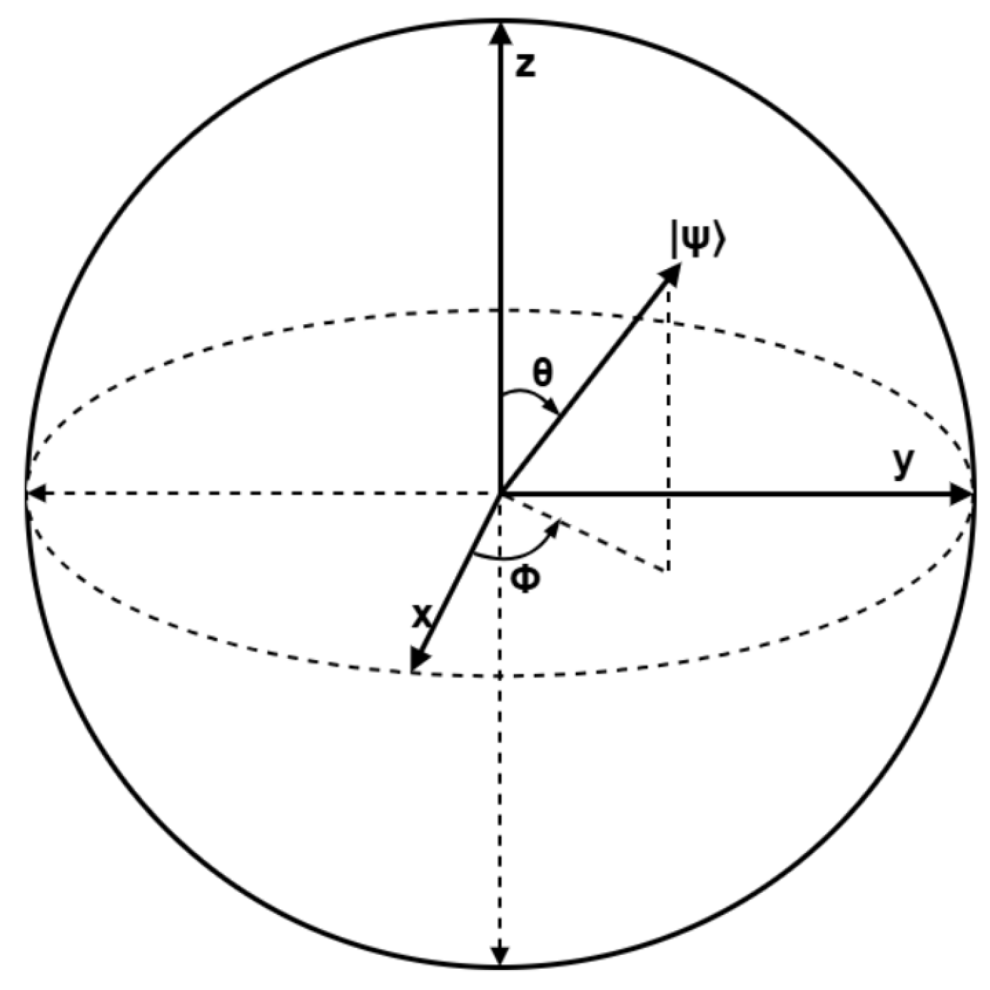
Figure 2.
VQC with a – CNOT – structure.
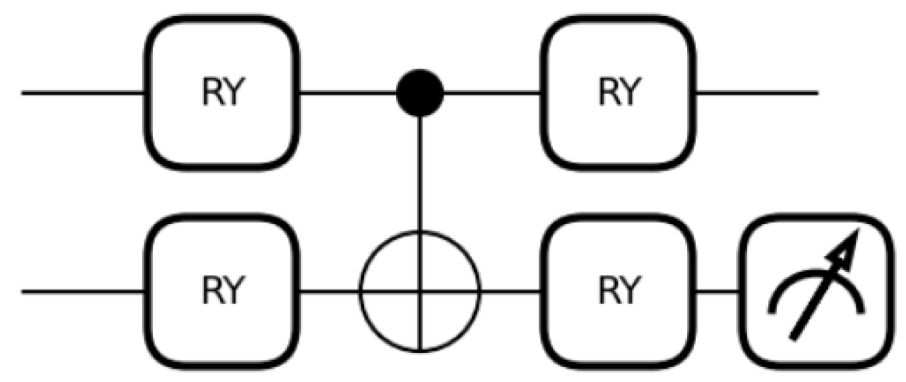
Figure 3.
Training loss vs. steps.
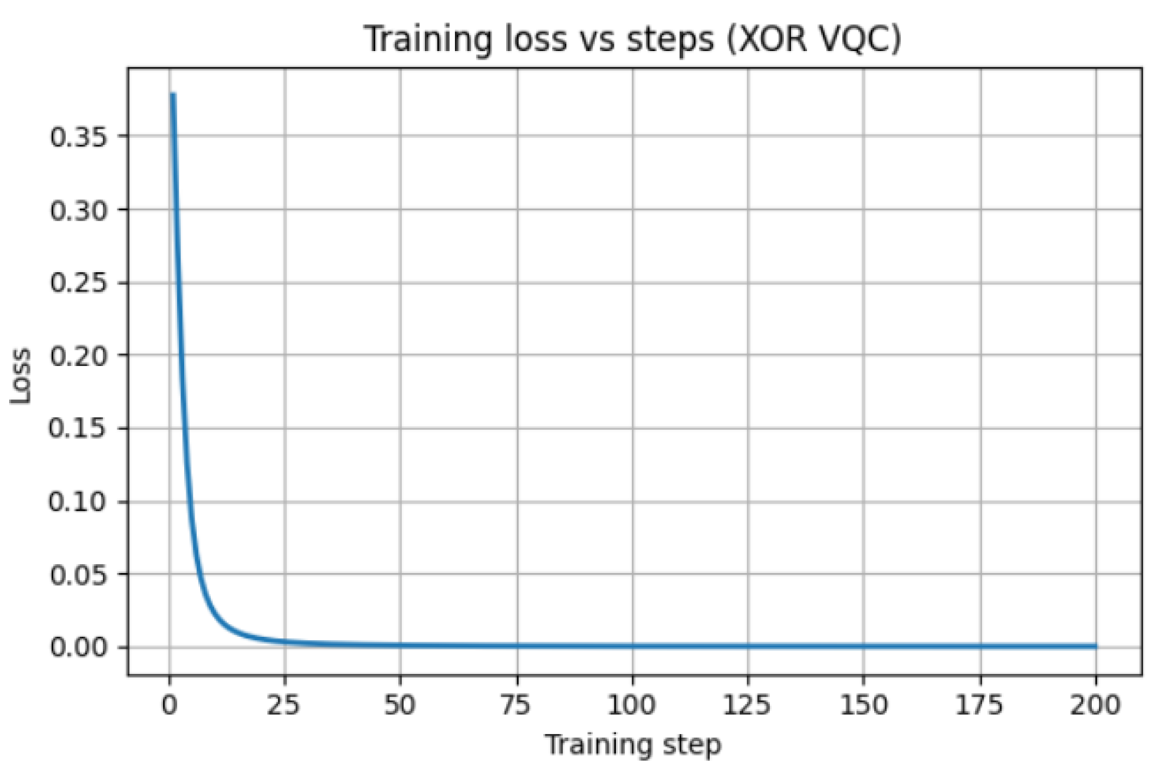
Figure 4.
Experimental results for input 00.
Figure 5.
Evaluation metrics for input 00.
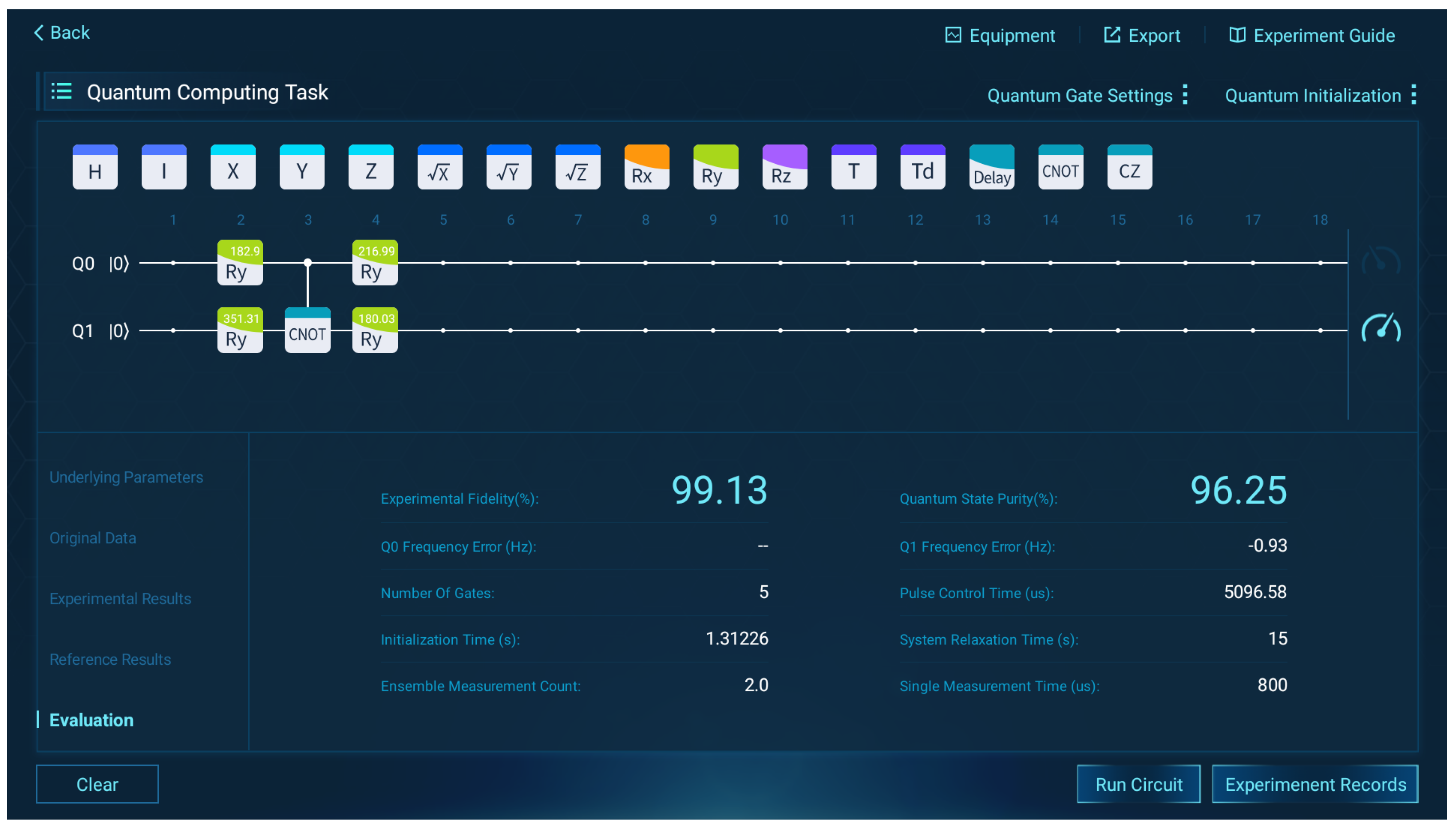
Figure 6.
XOR training: RY vs RX (with noise).
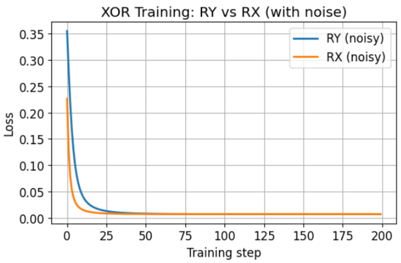
Figure 7.
XOR training: RY vs RX (noiseless).
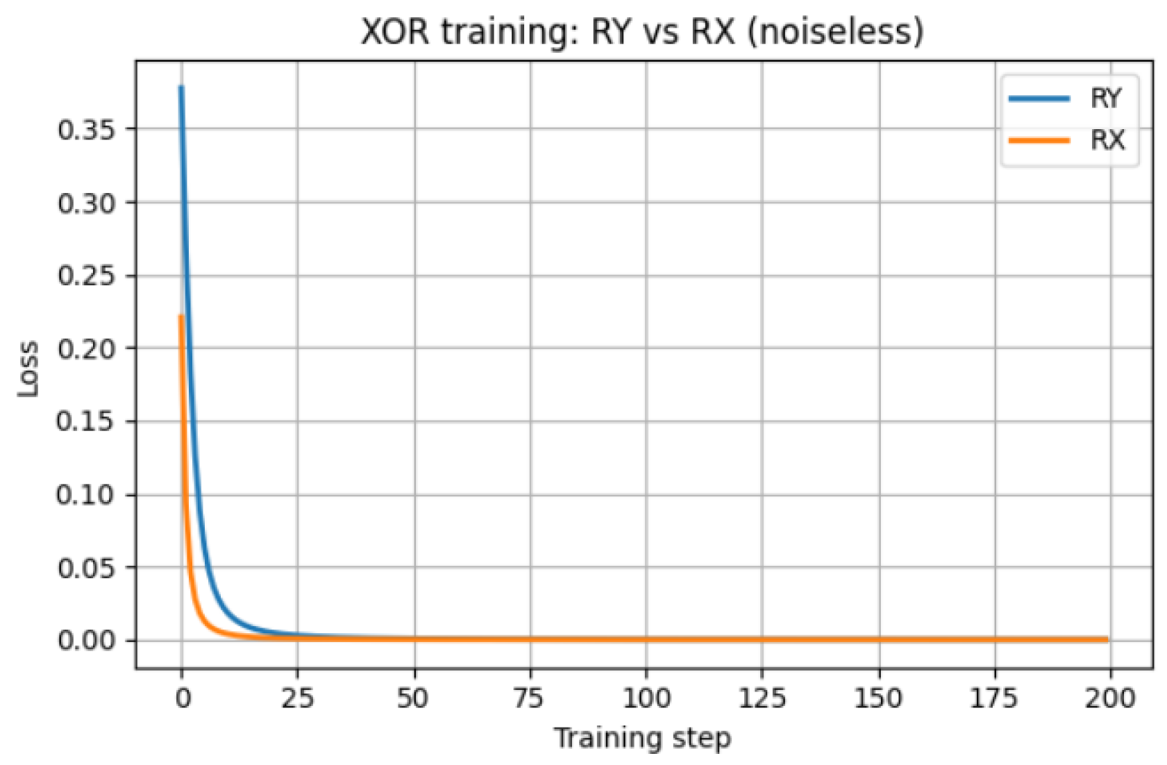
Figure 8.
Experimental results for input 00.
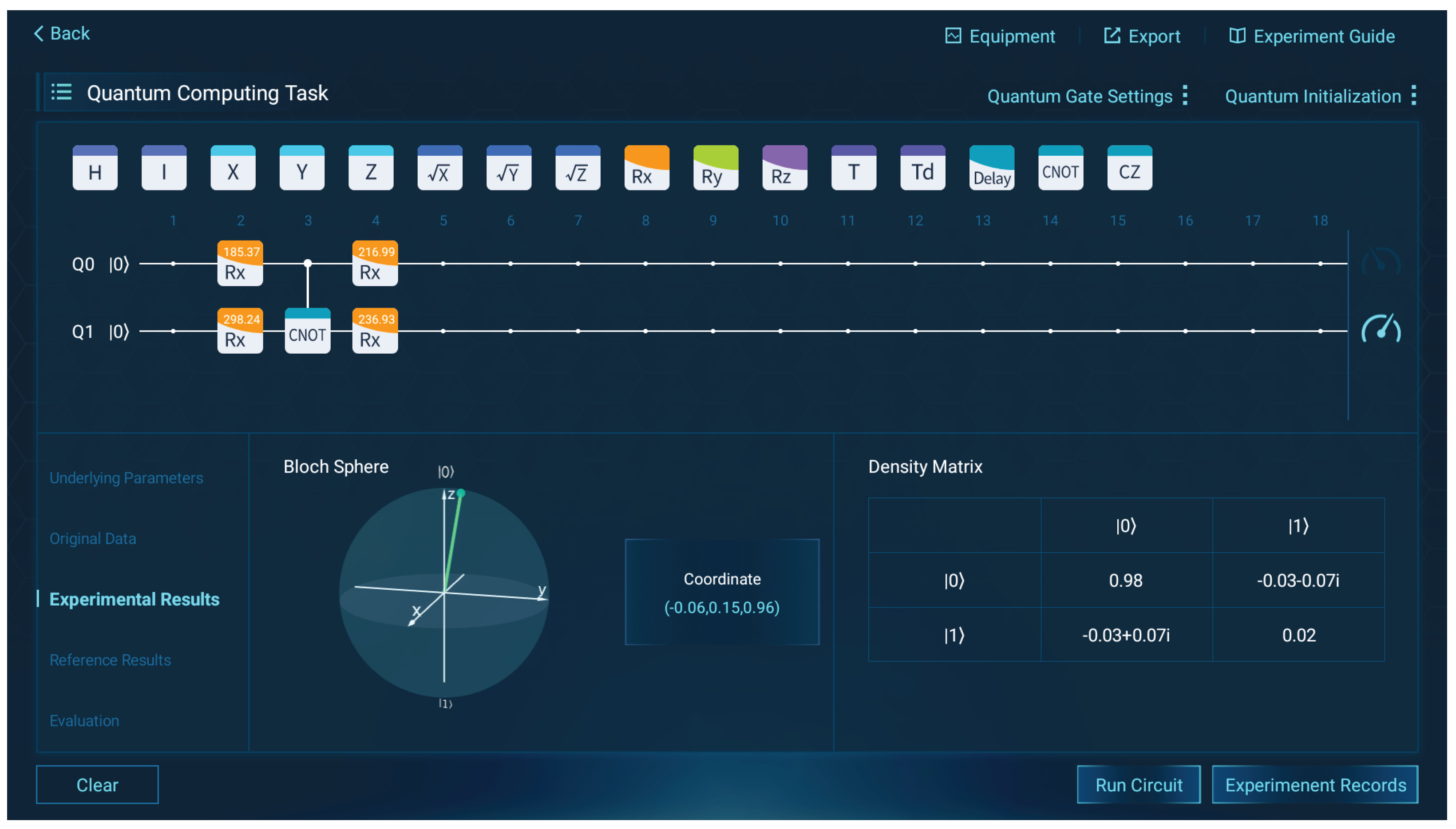
Figure 9.
Evaluation results for input 00.


Table 1.
Truth Table of the XOR Function.
| 0 | 0 | 0 |
| 0 | 1 | 1 |
| 1 | 0 | 1 |
| 1 | 1 | 0 |
Table 2.
Truth table of the CNOT gate.
| Control | Target | Output Control | Output Target |
|---|---|---|---|
| 0 | 0 | 0 | 0 |
| 0 | 1 | 0 | 1 |
| 1 | 0 | 1 | 1 |
| 1 | 1 | 1 | 0 |
Table 3.
Optimized rotation parameters in radians and degrees(Ry).
| Parameter | Radian (rad) | Degree (deg) |
|---|---|---|
| 3.192290 | 182.90 | |
| 6.131568 | 351.31 | |
| 3.787274 | 216.99 | |
| 3.142093 | 180.03 |
Table 4.
VQC performance on XOR truth table.
| Input | Target | VQC Output | Error |
|---|---|---|---|
| 00 | 0 | 0.0064 | 0.0064 |
| 01 | 1 | 0.9936 | 0.0064 |
| 10 | 1 | 0.9963 | 0.0037 |
| 11 | 0 | 0.0037 | 0.0037 |
Table 5.
Experimental and reference density matrices for all XOR inputs.
| Input | Basis | Experimental | Reference | ||
|---|---|---|---|---|---|
| 00 | 0.97 | 0.99 | 0.08 | ||
| 0.03 | 0.08 | 0.01 | |||
| 01 | 0.02 | 0.01 | |||
| 0.98 | 0.99 | ||||
| 10 | 0.02 | 0 | 0.01 | ||
| 0 | 0.98 | 0.99 | |||
| 11 | 0.95 | 0.99 | |||
| 0.05 | 0.01 | ||||
Table 6.
Fidelity and purity of four experimental runs(Ry).
| Input | Fidelity (%) | Purity (%) |
|---|---|---|
| 00 | 97.90 | 91.43 |
| 01 | 98.84 | 95.17 |
| 10 | 99.54 | 97.80 |
| 11 | 99.13 | 96.25 |
Table 7.
Final Loss Comparison Between RY and RX Circuits.
| Circuit | Loss (No Noise) | Loss (With Noise) |
|---|---|---|
| RY | ||
| RX |
Table 8.
Optimized rotation parameters in radians and degrees(Rx).
| Parameter | Radian (rad) | Degree (deg) |
|---|---|---|
| 3.235376 | 185.37 | |
| 5.205278 | 298.24 | |
| 3.787274 | 216.99 | |
| 4.135212 | 236.93 |
Table 9.
Experimental and reference density matrices for all XOR inputs(Rx).
| Input | Basis | Experimental | Reference | ||
|---|---|---|---|---|---|
| 00 | 0.98 | 1 | |||
| 0.02 | 0 | ||||
| 01 | 0.01 | 0 | |||
| 0.99 | 1 | ||||
| 10 | 0.01 | 0 | |||
| 0.99 | 1 | ||||
| 11 | 0.96 | 1 | |||
| 0.04 | 0 | ||||
Table 10.
Fidelity and purity of four experimental runs(Rx).
| Input | Fidelity (%) | Purity (%) |
|---|---|---|
| 00 | 99.59 | 96.92 |
| 01 | 99.58 | 100 |
| 10 | 99.34 | 100 |
| 11 | 98.89 | 92.78 |
Table 11.
Average fidelity and purity of RX and RY circuits.
| Metric | RX | RY |
|---|---|---|
| Average fidelity | 99.35% | 98.85% |
| Average purity | 97.43% | 95.16% |
Disclaimer/Publisher’s Note: The statements, opinions and data contained in all publications are solely those of the individual author(s) and contributor(s) and not of MDPI and/or the editor(s). MDPI and/or the editor(s) disclaim responsibility for any injury to people or property resulting from any ideas, methods, instructions or products referred to in the content. |
© 2026 by the authors. Licensee MDPI, Basel, Switzerland. This article is an open access article distributed under the terms and conditions of the Creative Commons Attribution (CC BY) license.
Copyright: This open access article is published under a Creative Commons CC BY 4.0 license, which permit the free download, distribution, and reuse, provided that the author and preprint are cited in any reuse.


