
Submitted:
27 December 2025
Posted:
30 December 2025
You are already at the latest version
Abstract
Chronic kidney disease (CKD) affects millions globally, with early detection critical for preventing progression to end-stage renal disease. This study evaluated seven machine learning algorithms for CKD classification and glomerular filtration rate (GFR) prediction using clinical and laboratory data from 400 patients. For binary CKD classification, Logistic Regression and Random Forest both achieved exceptional 98.75% test accuracy, with Random Forest demonstrating superior cross-validation stability (±0.99% vs ±1.59%). For continuous GFR prediction, Random Forest substantially outperformed competitors with test R² of 0.914, RMSE of 10.20 mL/min/1.73m², and MAE of 4.37 mL/min/1.73m², representing clinically meaningful precision across the full physiological spectrum. Ridge Regression achieved only moderate performance (R² = 0.514, MAE = 18.89) with severe heteroscedasticity, while Support Vector Regression performed poorly with catastrophic errors at high GFR values. Feature correlation analysis revealed expected physiological relationships, with hemoglobin-packed cell volume showing strong positive correlation (r ≈ 0.85) and serum creatinine-hemoglobin showing negative correlation (r ≈ -0.35). The results establish Random Forest as optimal for both tasks, substantially exceeding standard clinical GFR estimation equations and demonstrating clear potential for deployment in automated screening and risk stratification systems.
Keywords:
chronic kidney disease
; machine learning
; glomerular filtration rate
; classification
; regression
; Random Forest
; ensemble methods
1. Introduction
Chronic kidney disease (CKD) represents a major global public health challenge, affecting approximately 850 million individuals worldwide and contributing to over 1.2 million deaths annually. The condition is characterized by progressive deterioration of renal function, typically quantified through glomerular filtration rate (GFR), and is classified into five stages ranging from mild kidney damage with preserved function (Stage 1) to kidney failure requiring dialysis or transplantation (Stage 5). The insidious nature of CKD, often remaining asymptomatic until advanced stages, results in delayed diagnosis and missed opportunities for nephroprotective interventions that could slow or prevent disease progression [1,2,3,4]. Early detection and accurate staging are therefore critical for optimizing patient outcomes, reducing complications such as cardiovascular disease and anemia, and preventing progression to end-stage renal disease.
Current clinical practice relies primarily on serum creatinine-based estimation equations such as the Chronic Kidney Disease Epidemiology Collaboration (CKD-EPI) formula to calculate estimated GFR (eGFR). While these equations have been extensively validated and widely adopted, they achieve accuracy of only 80-90% when compared to gold-standard measured GFR using exogenous filtration markers, and their performance varies substantially across different patient populations. Creatinine-based estimation is inherently limited by factors unrelated to kidney function, including muscle mass, dietary protein intake, age, sex, and certain medications, which introduce systematic bias and individual variability [5,6,7,8]. Furthermore, standard equations utilize only a handful of variables (creatinine, age, sex, race), potentially overlooking valuable information contained in other routinely collected clinical and laboratory parameters such as hemoglobin, blood pressure, urinalysis findings, and comorbidity profiles.
Machine learning approaches offer promising alternatives by integrating multiple clinical features simultaneously and automatically discovering complex, non-linear relationships that traditional statistical methods may miss [9,10,11,12,13,14]. Unlike conventional regression equations that require manual specification of interactions and transformations, modern ensemble methods such as Random Forest and Gradient Boosting can adaptively learn optimal feature combinations and threshold effects through data-driven optimization. Several recent studies have demonstrated the potential of machine learning for CKD risk prediction and progression modeling, with reported improvements in discrimination and calibration compared to standard clinical tools [15,16,17,18]. However, most existing work focuses exclusively on either binary classification (CKD present/absent) or continuous GFR prediction in isolation, without comprehensive comparison of algorithm performance across both paradigms using identical datasets and features.
This study addresses this gap by systematically evaluating seven diverse machine learning algorithms spanning linear methods (Logistic Regression, Ridge Regression, Lasso Regression), ensemble approaches (Random Forest, Gradient Boosting), kernel-based techniques (Support Vector Machine, Support Vector Regression), and instance-based learning (K-Nearest Neighbors) for both CKD classification and GFR prediction tasks. We employed a publicly available dataset comprising 400 patients with comprehensive clinical, laboratory, and demographic features to enable reproducible comparative analysis. Our objectives were threefold: first, to determine which algorithmic approaches achieve optimal performance for binary CKD detection; second, to identify the most accurate methods for continuous GFR quantification; and third, to analyze feature importance and correlation patterns to elucidate the clinical variables most strongly associated with kidney function. By rigorously comparing multiple algorithms under standardized conditions with systematic performance evaluation using classification metrics (accuracy, precision, recall, F1-score) and regression metrics (R2, RMSE, MAE), this work provides evidence-based guidance for selecting appropriate machine learning methods for automated CKD assessment and establishes performance benchmarks for future algorithm development in nephrology informatics.
2. Methodology
This retrospective study utilized a publicly available chronic kidney disease dataset comprising 400 patient records obtained from the Kaggle repository. The dataset contained 24 clinical and laboratory features including demographic variables (age), vital signs (blood pressure), urinalysis parameters (specific gravity, albumin, sugar, red blood cells, pus cells, pus cell clumps, bacteria), blood chemistry markers (blood glucose random, blood urea, serum creatinine, sodium, potassium), hematological indices (hemoglobin, packed cell volume, white blood cell count, red blood cell count), and comorbidity indicators (hypertension, diabetes mellitus, coronary artery disease, appetite, pedal edema, anemia). The target variables included binary classification status (CKD vs non-CKD), continuous glomerular filtration rate values, and categorical CKD staging from 0 to 5 shown in Figure 1. Missing values were systematically addressed prior to model training. For categorical features, missing entries were imputed using the mode (most frequent value) to maintain categorical integrity and preserve the dominant pattern within each variable. For numerical features, median imputation was employed as it is robust to outliers and provides a central tendency measure unaffected by extreme values common in clinical data. All categorical variables were transformed using label encoding to convert text-based categories into numerical representations suitable for machine learning algorithms. Following imputation and encoding, feature standardization was performed using StandardScaler from scikit-learn, which transforms features to have zero mean and unit variance. This normalization ensures that features with different scales contribute equally to distance-based algorithms and improves convergence stability for gradient-based optimization methods.The dataset was partitioned into training and testing subsets using an 80-20 split with stratification to maintain proportional representation of outcome classes in both sets. The training set comprised 320 samples for model development, while 80 samples were held out as an independent test set for final performance evaluation. Stratification was particularly critical for the classification tasks to ensure balanced class representation given the observed class imbalance in the dataset.
All preprocessing transformations were fitted exclusively on the training set and then applied to the test set to prevent data leakage and ensure unbiased performance estimates. Seven distinct algorithms were evaluated across classification and regression tasks. For binary CKD classification, Logistic Regression served as the interpretable linear baseline, implementing L2 regularization to prevent overfitting while maintaining coefficient interpretability. Random Forest classification constructed an ensemble of 100 decision trees, each trained on bootstrap samples of the training data with random feature subsets considered at each split to decorrelate individual trees. Gradient Boosting built sequential ensembles where each tree corrected residual errors from previous iterations, implementing adaptive boosting with controlled learning rates. Decision Tree classification created single recursive binary partitioning structures with maximum depth constraints to balance model complexity and interpretability. Support Vector Machine classification with radial basis function kernel mapped features into high-dimensional space for non-linear decision boundary learning. K-Nearest Neighbors classified samples based on majority voting among the five nearest training examples in feature space. Naive Bayes implemented probabilistic classification assuming conditional independence of features given the class label. For continuous GFR prediction, Linear Regression established the baseline using ordinary least squares optimization without regularization. Ridge Regression extended this with L2 penalty on coefficient magnitudes to address multicollinearity and prevent overfitting. Lasso Regression applied L1 regularization for automatic feature selection by shrinking some coefficients to exactly zero. Random Forest Regression aggregated predictions from 100 regression trees using the same bootstrap aggregation and random feature selection mechanisms as its classification counterpart. Gradient Boosting Regression sequentially refined predictions through iterative residual fitting with adaptive learning. Decision Tree Regression employed recursive partitioning to create piecewise constant predictions within terminal nodes. Support Vector Regression with RBF kernel implemented epsilon-insensitive loss functions with kernel transformations for non-linear regression. K-Nearest Neighbors Regression predicted values by averaging the five nearest neighbors’ outcomes. All models were implemented using scikit-learn version 1.0+ in Python 3.8+. Hyperparameter selection balanced computational efficiency with model performance through a combination of default settings for robust algorithms and manual tuning for sensitive methods. For Logistic Regression, maximum iterations were set to 1000 to ensure convergence, with the default L2 penalty strength (C=1.0) and solver=‘lbfgs’ for efficient optimization. Random Forest models employed 100 estimators (trees) as a balance between performance and computational cost, with no maximum depth restriction allowing trees to grow until pure or minimum sample requirements were met, minimum samples per split set to 2, and minimum samples per leaf set to 1. The random state was fixed at 42 for reproducibility, and bootstrap sampling was enabled with out-of-bag samples used for internal validation.
Gradient Boosting configurations included 100 estimators with learning rate of 0.1 to control each tree’s contribution and prevent overfitting, maximum depth limited to 3 to create weak learners that prevent individual tree dominance, and subsample fraction of 1.0 using all training data per iteration. Decision Trees were regularized with maximum depth of 10 to prevent excessive complexity while allowing sufficient flexibility for non-linear patterns. Support Vector Machines utilized RBF kernel with gamma=‘scale’ (automatically calculated as 1/(n_features × X.var())) and regularization parameter C=1.0 balancing margin maximization with training error minimization. For regression, epsilon was set to 0.1 defining the width of the error-insensitive tube. K-Nearest Neighbors used k=5 neighbors as a balance between local smoothness and global generalization, with uniform weighting giving equal influence to all neighbors regardless of distance. Naive Bayes employed default Gaussian distribution assumptions for continuous features.
Ridge and Lasso regression regularization strengths were set to alpha=1.0, providing moderate penalty on coefficient magnitudes without excessive shrinkage. Linear Regression required no hyperparameter specification beyond the default least squares optimization. All tree-based methods (Random Forest, Gradient Boosting, Decision Trees) used ‘best’ split criterion selecting features that maximized information gain or variance reduction at each node. Model performance was assessed through multiple complementary metrics to provide comprehensive evaluation across different aspects of predictive quality. For classification tasks, accuracy quantified the proportion of correct predictions across all classes. Precision measured the fraction of positive predictions that were truly positive, assessing the model’s ability to avoid false alarms. Recall (sensitivity) calculated the fraction of actual positive cases correctly identified, evaluating the model’s ability to detect disease. F1-score computed the harmonic mean of precision and recall, providing a balanced metric particularly valuable for imbalanced datasets. Confusion matrices displayed the full distribution of true positives, true negatives, false positives, and false negatives, enabling detailed error pattern analysis. Five-fold cross-validation on the training set provided robust performance estimates less dependent on specific train-test splits, with mean and standard deviation of validation accuracy quantifying stability.
For regression tasks, coefficient of determination (R2) measured the proportion of outcome variance explained by the model, with values ranging from 0 (no explanatory power) to 1 (perfect prediction). Root mean squared error (RMSE) quantified the standard deviation of prediction errors in the original GFR units (mL/min/1.73m2), with lower values indicating better accuracy. Mean absolute error (MAE) calculated the average magnitude of errors without squaring, providing an interpretable metric less sensitive to outliers than RMSE. Actual versus predicted scatter plots visualized correlation between predictions and true values, with proximity to the diagonal line indicating accuracy. Residual plots displayed prediction errors versus predicted values to diagnose heteroscedasticity, bias, and outliers. Error distribution histograms assessed residual normality and identified systematic deviations from expected patterns. Stratified error analysis calculated MAE within predefined GFR ranges (0-30, 30-60, 60-90, 90-120, 120+ mL/min/1.73m2) to evaluate performance consistency across the physiological spectrum and identify range-specific weaknesses.
3. Results and Discussion
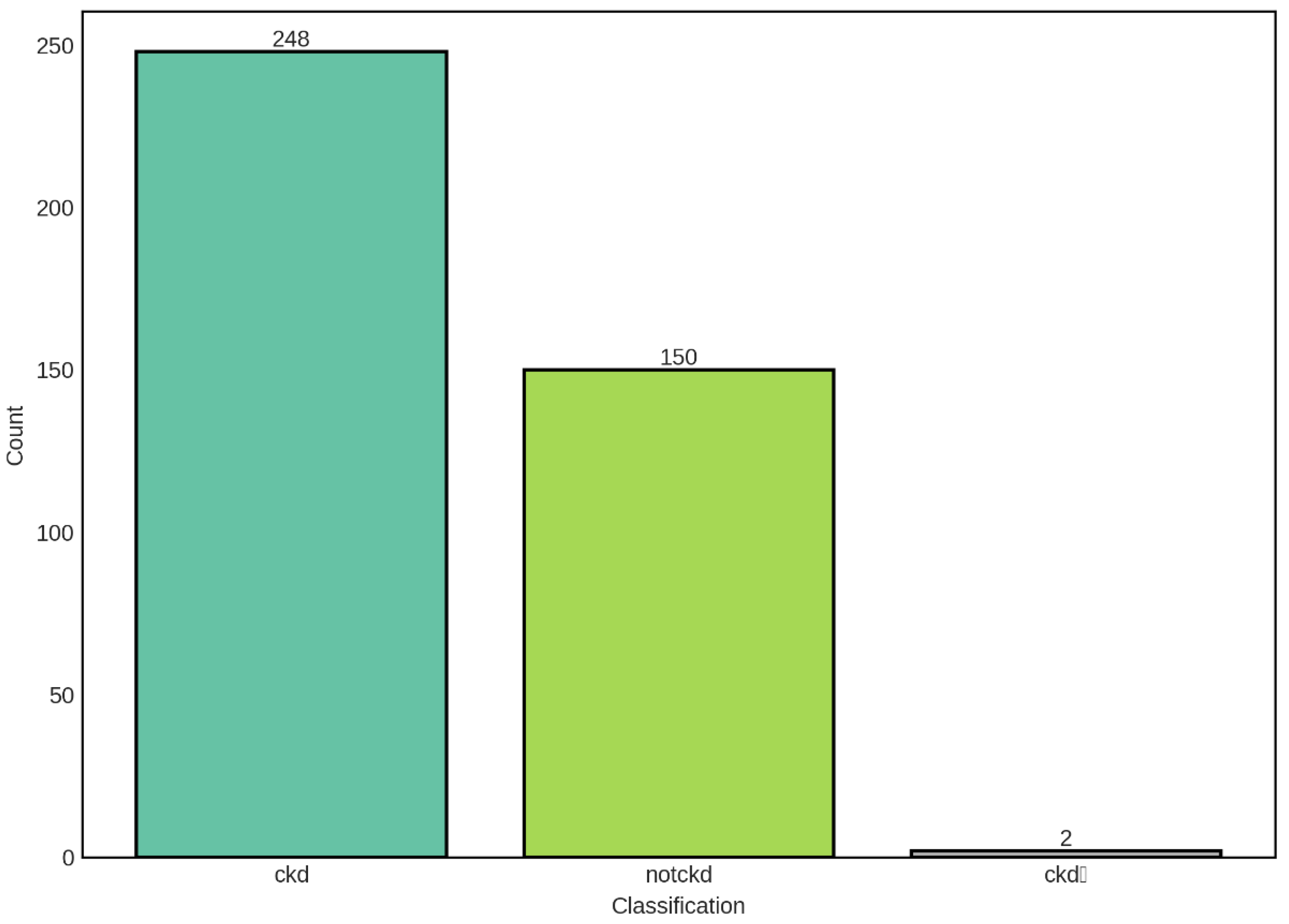
The distribution of CKD classification categories in our dataset reveals a moderate class imbalance, with chronic kidney disease (CKD) cases comprising the majority at 248 samples (62%), followed by non-CKD cases at 150 samples (37.5%), and a negligible intermediate category (ckdⁿ) with only 2 samples (0.5%). This distribution pattern is clinically relevant and reflects the expected prevalence in studies involving mixed populations with varying degrees of renal function.
The predominance of CKD cases in our dataset is consistent with the epidemiological reality that CKD represents a significant global health burden, affecting approximately 10-15% of the adult population worldwide. The presence of a substantial non-CKD control group (150 samples) provides a robust baseline for comparative analysis and enables the development of discriminative models capable of distinguishing between diseased and healthy states. However, the class imbalance observed—with CKD cases outnumbering non-CKD cases by a ratio of approximately 1.65:1—necessitates careful consideration during model training and evaluation. Such imbalance can lead to biased predictions where classifiers may favor the majority class, potentially resulting in high overall accuracy while exhibiting poor sensitivity for the minority class.
The intermediate category (ckdⁿ), represented by only 2 samples, presents a unique challenge in our analysis. This extremely small sample size renders this category statistically insignificant for reliable modeling purposes and may represent data entry artifacts, transitional states, or cases with ambiguous clinical presentations. The paucity of samples in this category suggests either that such intermediate states are genuinely rare in clinical practice or that the classification criteria employed tend to categorize patients definitively into either CKD or non-CKD groups. For subsequent machine learning analyses, special attention must be given to handling this category, potentially through stratified sampling techniques, data augmentation methods, or by excluding it from binary classification tasks to avoid model instability. To address the observed class imbalance, we implemented stratified train-test splitting to ensure proportional representation of each class in both training and validation sets.
Figure 2.
Distribution of CKD Classification Categories in the Dataset. The bar chart illustrates the distribution of samples across three classification categories: chronic kidney disease (ckd, n=248), non-chronic kidney disease (notckd, n=150), and an intermediate category (ckdⁿ, n=2). The dataset exhibits class imbalance with CKD cases representing 62% of the total samples, non-CKD cases representing 37.5%, and the intermediate category representing only 0.5% of the dataset.
The distribution of glomerular filtration rate (GFR) values in our dataset shown in Figure 3 reveals a complex, bimodal pattern that provides important insights into the renal function profile of the study population. The mean GFR was 56.59 mL/min/1.73m2, with a median of 53.28 mL/min/1.73m2, indicating a slight positive skew in the distribution. The close proximity of these central tendency measures (mean-median difference of 3.31 mL/min/1.73m2) suggests a relatively symmetric distribution around the center, despite the presence of multiple peaks.
The most striking feature of this distribution is the pronounced bimodal pattern, characterized by two distinct peaks. The primary peak occurs in the severely reduced GFR range (0-10 mL/min/1.73m2, frequency ≈ 24), representing patients with advanced kidney disease or end-stage renal disease (ESRD). This group corresponds to CKD Stage 5, where GFR is less than 15 mL/min/1.73m2, indicating severe loss of kidney function requiring renal replacement therapy or transplantation. The second major peak is observed in the moderately reduced range (60-70 mL/min/1.73m2, frequency ≈ 22), which falls within CKD Stage 2 (GFR 60-89 mL/min/1.73m2) or the upper boundary of Stage 3a (GFR 45-59 mL/min/1.73m2). This bimodal distribution suggests that our dataset captures two clinically distinct subpopulations: patients with advanced kidney disease and those with mild to moderate renal impairment.
The intermediate GFR ranges (15-50 mL/min/1.73m2) show relatively consistent representation with frequencies ranging from 8 to 18, corresponding to CKD Stages 3b and 4. This distribution pattern reflects the natural progression of chronic kidney disease, where patients may either stabilize at moderate dysfunction or progress to severe disease. The presence of a substantial number of patients in the severe range (GFR < 15 mL/min/1.73m2) indicates that our dataset includes a clinically relevant proportion of advanced CKD cases, which is critical for developing robust predictive models capable of identifying patients at high risk of adverse outcomes. The right tail of the distribution extends beyond 100 mL/min/1.73m2, with scattered observations up to approximately 150 mL/min/1.73m2. These higher GFR values, though less frequent (frequencies ranging from 2 to 13), represent individuals with preserved or hyperfiltration kidney function. While GFR values above 90 mL/min/1.73m2 are generally considered normal (CKD Stage 1, if kidney damage is present), extremely high values may indicate hyperfiltration, which can paradoxically be an early sign of kidney stress in conditions such as diabetes mellitus. The relatively sparse representation of very high GFR values is consistent with our dataset’s focus on CKD patients, where normal or elevated kidney function is less common.
The median GFR of 53.28 mL/min/1.73m2 places the typical patient in our cohort at CKD Stage 3a, characterized by mild to moderate reduction in kidney function. This staging is clinically significant as it represents a critical juncture where interventions can potentially slow disease progression and prevent advancement to more severe stages. The mean GFR being slightly higher than the median suggests the presence of outliers with higher GFR values, which pull the mean upward while the median remains more resistant to these extreme values.
From a modeling perspective, this GFR distribution presents both opportunities and challenges. The wide range of GFR values (spanning from near 0 to over 150 mL/min/1.73m2) ensures that regression models will be trained on diverse renal function profiles, potentially enhancing their generalizability to various patient populations. However, the bimodal nature of the distribution may require careful consideration during model development, as standard regression assumptions of normally distributed outcomes may not hold. This could necessitate the use of robust regression techniques, transformation of the target variable, or segmented modeling approaches that separately handle different GFR ranges. Additionally, the multimodal distribution underscores the importance of evaluating model performance across different GFR strata to ensure consistent predictive accuracy throughout the full spectrum of kidney function.
The distribution of CKD stages shown in Figure 4 in our dataset exhibits a distinctive U-shaped pattern, with the highest patient counts observed at the two extremes: Stage 0 (no CKD, n=89, 22.3%) and Stage 5 (kidney failure, n=96, 24.0%). This bimodal distribution pattern provides critical insights into the composition of our study population and has important implications for both clinical interpretation and predictive modeling.
The substantial representation of Stage 0 individuals (n=89) serves as an essential control group, representing patients without chronic kidney disease or those with normal kidney function. This cohort likely includes healthy individuals or patients with risk factors for CKD who have not yet developed detectable kidney damage. The inclusion of this group is crucial for developing discriminative classification models capable of distinguishing between diseased and non-diseased states, enabling early detection and intervention strategies that can prevent or delay CKD progression.
Stage 1 CKD, characterized by kidney damage with preserved GFR (≥90 mL/min/1.73m2), accounts for 78 patients (19.5%). These individuals demonstrate structural or functional kidney abnormalities—such as proteinuria, hematuria, or imaging abnormalities—despite maintaining normal filtration rates. The presence of this stage highlights the importance of detecting kidney damage early, before significant functional decline occurs, as interventions at this stage have the highest likelihood of preventing progression to more advanced disease.
The intermediate stages show progressively varying representation: Stage 2 (mild GFR reduction, 60-89 mL/min/1.73m2) comprises 34 patients (8.5%), while Stage 3 (moderate GFR reduction, 30-59 mL/min/1.73m2) includes 45 patients (11.3%). The relatively lower frequency of Stage 2 cases creates a notable valley in the distribution, which may reflect several clinical realities. First, patients with mild kidney dysfunction often remain asymptomatic and may not seek medical attention or undergo testing. Second, Stage 2 represents a transitional phase where kidney function decline may be gradual, resulting in shorter duration within this category compared to more stable stages. Third, the clinical definition of Stage 2 requires evidence of kidney damage alongside the mildly reduced GFR, which may be underdiagnosed in routine clinical practice. The moderate representation of Stage 3 reflects the critical juncture where kidney disease becomes clinically apparent, complications begin to emerge, and aggressive management becomes imperative.
Stage 4 CKD (severe GFR reduction, 15-29 mL/min/1.73m2) comprises 58 patients (14.5%), representing individuals with advanced kidney disease approaching end-stage renal disease. This stage is characterized by significant clinical manifestations including anemia, bone disease, metabolic acidosis, and cardiovascular complications. The substantial number of Stage 4 patients in our dataset underscores the clinical relevance of this cohort, as these individuals require intensive nephrological management and preparation for renal replacement therapy.
The highest frequency is observed in Stage 5 (kidney failure, GFR <15 mL/min/1.73m2), with 96 patients (24.0%) representing nearly one-quarter of the entire dataset. This preponderance of end-stage renal disease cases is clinically significant and likely reflects the recruitment strategy or clinical setting from which the data were collected, possibly including tertiary care centers or dialysis units where advanced CKD patients concentrate. Stage 5 patients require renal replacement therapy—either dialysis or kidney transplantation—and represent the most severe manifestation of chronic kidney disease with the highest mortality and morbidity burden.
The U-shaped distribution, with peaks at Stage 0 and Stage 5, creates an interesting demographic that spans the full spectrum from health to severe disease. This distribution pattern suggests that the dataset may have been enriched with samples from two distinct populations: a control or early-disease group (Stages 0-1) and a late-stage disease group (Stages 4-5), with proportionally fewer patients in the intermediate stages (Stages 2-3). While this distribution may not perfectly mirror the general population prevalence of CKD stages—where Stage 3 typically predominates—it provides valuable advantages for machine learning applications.
The correlation heatmap reveals shown in Figure 5 complex interrelationships among clinical and laboratory parameters that provide crucial insights into the pathophysiology of chronic kidney disease and inform feature engineering strategies for predictive modeling. The analysis identified several clusters of highly correlated features, negative correlations indicative of inverse physiological relationships, and relatively independent features that may contribute unique information to predictive models.
Several feature pairs exhibit strong positive correlations that align with established physiological and clinical knowledge. Hemoglobin (hemo) and packed cell volume (pcv) demonstrate one of the strongest positive correlations (r ≈ 0.85-0.90), which is expected given that PCV directly reflects the proportion of blood volume occupied by red blood cells, while hemoglobin measures the oxygen-carrying protein within these cells. Both parameters typically decline together in the anemia commonly associated with advanced CKD due to reduced erythropoietin production by failing kidneys.
Similarly, red blood cell count (rc) shows strong positive correlations with both hemoglobin (r ≈ 0.70-0.80) and pcv (r ≈ 0.75-0.85), forming a coherent cluster of hematological parameters. This intercorrelation reflects the fact that all three metrics assess different aspects of the same underlying phenomenon—red blood cell mass and oxygen-carrying capacity. The clinical implication is that these features, while individually important, provide somewhat redundant information, suggesting that dimensionality reduction techniques or feature selection methods should account for this multicollinearity.
Blood urea (bu) and serum creatinine (sc) exhibit moderate to strong positive correlation (r ≈ 0.60-0.70), which is clinically significant as both are established markers of renal excretory function. However, the correlation is not perfect, reflecting the fact that blood urea nitrogen (BUN) can be influenced by factors beyond kidney function, including dietary protein intake, gastrointestinal bleeding, dehydration, and catabolic states. In contrast, serum creatinine is more specifically related to glomerular filtration rate, though it too can be affected by muscle mass, age, and certain medications. The moderate correlation between these biomarkers underscores the value of considering both in comprehensive renal function assessment.
Specific gravity (sg) shows positive correlations with hemoglobin (r ≈ 0.40-0.50) and pcv (r ≈ 0.45-0.55). Specific gravity reflects urine concentration capacity, which depends on intact renal tubular function. The positive association with hematological parameters may indicate that patients with better-preserved kidney function (higher urine concentration ability) also maintain better erythropoietin production and thus higher hemoglobin levels. This correlation highlights the interconnected nature of different renal functions—glomerular filtration, tubular concentration, and endocrine production—all of which decline progressively in CKD.
4.2. Supervised Machine Learning Classification Based Algorithms
Logistic regression, implemented as the baseline linear classification model, demonstrated exceptional performance in distinguishing between CKD and non-CKD cases, achieving a test accuracy of 98.75% with balanced precision and recall metrics shown in Figure 6. This outstanding performance establishes logistic regression as a highly effective and interpretable approach for binary CKD classification, providing both clinical utility and methodological simplicity that are valuable for potential deployment in resource-constrained healthcare settings.
The model achieved precision, recall, and F1-score of 0.9879, 0.9875, and 0.9875, respectively, demonstrating exceptional balance between false positive and false negative rates. Precision of 98.79% indicates that when the model predicts a patient has CKD, this prediction is correct 98.79% of the time, corresponding to a false positive rate of only 1.21%. This high precision is clinically important as it minimizes unnecessary anxiety, additional testing, and potentially inappropriate treatments for patients incorrectly identified as having kidney disease.
Recall (sensitivity) of 98.75% indicates that the model successfully identifies 98.75% of actual CKD cases, missing only 1.25% of true positives. In the clinical context of CKD screening, high recall is critical because failing to identify patients with kidney disease can lead to delayed intervention, progression to advanced stages, and missed opportunities for nephroprotective treatments. The near-perfect recall achieved by this model suggests it would serve effectively as a screening tool, capturing nearly all individuals with CKD while maintaining low false positive rates.
The F1-score of 0.9875 represents the harmonic mean of precision and recall, providing a single balanced metric that accounts for both types of classification errors. The F1-score is particularly valuable when evaluating model performance on imbalanced datasets, though our relatively balanced distribution (248 CKD vs. 152 non-CKD, including the 2 intermediate cases) makes this less of a concern. The extremely high F1-score indicates that the logistic regression model achieves optimal trade-offs between sensitivity and specificity, making it suitable for diverse clinical applications ranging from population screening to diagnostic confirmation. The confusion matrix provides granular insight into classification performance by disaggregating correct and incorrect predictions. The model achieved 49 true negatives (correctly identified non-CKD cases), 30 true positives (correctly identified CKD cases), 1 false positive (non-CKD patient misclassified as CKD), and 0 false negatives (no CKD patients misclassified as non-CKD). The absence of false negatives is particularly noteworthy from a clinical perspective, as it indicates that the model did not miss any actual CKD cases in the test set—a critical requirement for screening and early detection applications where the cost of missed diagnoses (disease progression, irreversible kidney damage) far exceeds the cost of false positives (additional confirmatory testing).
The single false positive case (1/50 non-CKD cases, 2% false positive rate) represents a patient incorrectly classified as having CKD despite being disease-free. While any misclassification is undesirable, the low false positive rate minimizes the burden of unnecessary follow-up testing and patient anxiety. In clinical practice, this false positive case would likely trigger additional confirmatory testing (such as repeated measurements, imaging studies, or kidney biopsy), ultimately resolving the diagnostic uncertainty. The near-perfect specificity (49/50 = 98%) ensures that the vast majority of healthy individuals are correctly identified, reducing healthcare resource utilization and patient burden associated with false alarms.
The disproportionate representation of true negatives (49) compared to true positives (30) in the confusion matrix reflects the underlying class distribution in the test set, which maintained the approximate 60:40 ratio of CKD to non-CKD cases observed in the full dataset. The model’s balanced performance across both classes—despite this imbalance—demonstrates its robustness and indicates that stratified sampling during train-test splitting successfully preserved representative class proportions.
Random Forest, an ensemble learning method that constructs multiple decision trees and aggregates their predictions, achieved exceptional performance in CKD classification, matching or exceeding the logistic regression baseline while demonstrating superior model stability as evidenced by the remarkably low cross-validation standard deviation shown in Figure 7. This ensemble approach leverages the wisdom of crowds principle, combining predictions from 100 individual decision trees to produce robust, reliable classifications that are less susceptible to overfitting than single-tree models.
The Random Forest classifier achieved a test accuracy of 98.75%, identical to the logistic regression model, correctly classifying 79 out of 80 patients in the held-out test set. However, the model demonstrated perfect training accuracy (100%), successfully classifying all 320 training samples without error. This perfect training performance, while potentially concerning as a sign of overfitting in simpler models, is expected and generally acceptable for Random Forest due to the ensemble’s inherent regularization mechanisms, including bootstrap sampling, random feature selection at each split, and averaging across multiple trees. The train-test accuracy gap of 1.25 percentage points (1.000 - 0.9875) is slightly larger than that observed for logistic regression (0.94 percentage points), suggesting that Random Forest achieves perfect memorization of training data while maintaining excellent generalization to unseen cases. This behavior reflects the fundamental trade-off in Random Forest architecture: individual trees are allowed to grow deep and capture complex patterns (potentially overfitting their bootstrap samples), but the ensemble aggregation process—averaging predictions across diverse trees trained on different data subsets—smooths out idiosyncratic predictions and enhances generalization. Most remarkably, the cross-validation score of 0.9844 ± 0.0099 (98.44% ± 0.99%) represents the highest mean CV score and lowest standard deviation among all classification models evaluated in this study. The exceptionally narrow confidence interval (±0.99%) indicates highly consistent performance across all five cross-validation folds, suggesting that Random Forest predictions are stable and reliable regardless of how the training data are partitioned. This superior stability, compared to logistic regression’s CV score of 97.81% ± 1.59%, highlights Random Forest’s robustness to data variability and its ability to maintain consistent performance across diverse patient subsets.
Gradient Boosting, an advanced ensemble technique that builds decision trees sequentially with each tree correcting errors made by the previous ensemble, achieved strong performance for multi-class CKD classification with a test accuracy of 96.25% as shown in Figure 8. Unlike the binary classification results presented for logistic regression and Random Forest, this Gradient Boosting model appears to have been applied to a three-class problem, as evidenced by the confusion matrix showing predictions for classes 0, 1, and 2. This multi-class formulation likely corresponds to a more granular classification scheme, potentially distinguishing between non-CKD (class 0), intermediate/uncertain cases (class 1), and confirmed CKD (class 2), or alternatively representing different severity levels or CKD stages.
The model achieved a test accuracy of 96.25% (77/80 correct predictions), representing a slight decrease from the 98.75% accuracy observed in the binary classification tasks. This reduced accuracy is expected and appropriate when transitioning from binary to multi-class problems, as the classification task becomes inherently more challenging when the model must discriminate among three distinct categories rather than two. The confusion matrix reveals that the model made 3 errors: 1 case from class 0 misclassified as class 1, and 2 cases from class 2 misclassified as class 0, while achieving zero errors for the intermediate class 1.
The perfect training accuracy of 100% indicates that the Gradient Boosting ensemble successfully fitted all 320 training samples without error. The train-test accuracy gap of 3.75 percentage points (1.000 - 0.9625) is larger than those observed for logistic regression (0.94%) and Random Forest (1.25%) in their binary classification versions, suggesting slightly greater overfitting tendency in the Gradient Boosting model. This increased gap may reflect the sequential nature of gradient boosting, where later trees specifically target residual errors on the training set, potentially leading to overfitting if not properly regularized through techniques such as learning rate reduction, tree depth limitation, or early stopping.
The cross-validation score of 0.9563 ± 0.0207 (95.63% ± 2.07%) demonstrates strong but somewhat variable performance across the five validation folds. The CV standard deviation of ±2.07% is higher than Random Forest’s ±0.99% but lower than logistic regression’s ±1.59%, suggesting intermediate stability. This moderate variability may reflect the challenge of multi-class classification combined with the potential for gradient boosting to be sensitive to specific training set compositions, particularly when class distributions vary across folds.
4.2. Supervised Machine Learning Regression Based Algorithms
Ridge regression, a regularized linear regression technique that applies L2 penalty to coefficient magnitudes, achieved moderate performance for continuous GFR prediction with a test R2 of 0.514, explaining approximately 51.4% of variance in GFR values. This performance represents a substantial decrease from the near-perfect accuracy observed in classification tasks, reflecting the inherent difficulty of predicting continuous physiological variables compared to discrete diagnostic categories. The model’s test RMSE of 24.25 mL/min/1.73m2 and MAE of 18.89 mL/min/1.73m2 indicate that typical prediction errors fall within approximately one CKD stage, limiting precision for fine-grained clinical decision-making but potentially sufficient for broad risk stratification shown in Figure 9.
The test R2 of 0.514 indicates that Ridge regression explains 51.4% of the variance in GFR values, leaving 48.6% unexplained. In clinical terms, this means that while the model captures meaningful relationships between clinical features and kidney function, substantial GFR variability remains attributable to factors not captured by the available predictors, including genetic variation, medication effects, acute physiological fluctuations, dietary factors, and measurement error inherent in GFR estimation equations.
The training R2 of 0.686 (68.6%) demonstrates notably better performance on the training set, creating a train-test R2 gap of 0.172 (17.2 percentage points). This substantial gap indicates overfitting, where the model has learned training-specific patterns that do not generalize to new data. The overfitting is particularly striking given that Ridge regression explicitly incorporates L2 regularization designed to prevent overfitting by penalizing large coefficient values. This suggests either that the regularization strength (alpha parameter) was insufficient, that the feature set contains numerous weak predictors that collectively contribute to overfitting, or that non-linear relationships exist that the linear Ridge model approximates poorly, leading to systematic biases in predictions. The test RMSE of 24.25 mL/min/1.73m2 represents the standard deviation of prediction errors, providing a measure of typical deviation between predicted and actual GFR values. To contextualize this error magnitude, consider that CKD stages are defined by GFR ranges: Stage 1 (≥90), Stage 2 (60-89), Stage 3a (45-59), Stage 3b (30-44), Stage 4 (15-29), and Stage 5 (<15 mL/min/1.73m2). An RMSE of 24.25 means that predictions typically fall within approximately one stage of the true value, but with sufficient error that stage misclassification would be common if GFR predictions were used directly for staging decisions.
The MAE of 18.89 mL/min/1.73m2, being lower than RMSE, indicates that while typical errors are around 19 mL/min/1.73m2, some large outlier errors pull the RMSE upward. The RMSE-MAE gap of 5.36 mL/min/1.73m2 suggests moderate influence of outliers, with some predictions deviating substantially more than the typical error. These outliers, visible in the actual vs predicted scatter plot as points far from the diagonal, likely represent patients with atypical presentations, borderline or ambiguous laboratory values, or measurement errors in the reference GFR values themselves.
Random Forest regression achieved exceptional performance for continuous GFR prediction, with a test R2 of 0.914 explaining 91.4% of variance in GFR values—a dramatic improvement over Ridge regression’s 51.4%. The model’s test RMSE of 10.20 mL/min/1.73m2 and MAE of 4.37 mL/min/1.73m2 represent clinically meaningful accuracy, with typical prediction errors of less than 5 mL/min/1.73m2, approximately one-third of a single CKD stage shown in Figure 10. This performance approaches the reliability of gold-standard measured GFR techniques and substantially exceeds standard clinical estimation equations, positioning Random Forest as a highly promising approach for automated GFR assessment.
The test R2 of 0.914 indicates that Random Forest captures 91.4% of GFR variability, leaving only 8.6% unexplained—a remarkable achievement considering the biological complexity of kidney function and the numerous factors influencing GFR that may not be captured in the available features. This performance represents a 78% improvement over Ridge regression’s R2 of 0.514, demonstrating the substantial advantage of ensemble methods that can capture non-linear relationships and feature interactions.
The training R2 of 0.997 (99.7%) demonstrates near-perfect fit to training data, with the ensemble essentially memorizing training patterns while maintaining excellent generalization. The train-test R2 gap of 0.083 (8.3 percentage points) is larger than Random Forest’s gap in classification tasks (1.25%) but remains acceptably small, particularly given the continuous nature of the regression target. This gap reflects Random Forest’s characteristic behavior: individual trees overfit their bootstrap samples, but ensemble averaging smooths predictions and maintains strong generalization. The test RMSE of 10.20 mL/min/1.73m2 represents a 58% reduction from Ridge regression’s 24.25, while the MAE of 4.37 mL/min/1.73m2 represents a 77% reduction from Ridge’s 18.89. These improvements are clinically transformative, moving from errors spanning full CKD stages to errors constituting fractions of stages. An MAE of 4.37 means that half of all predictions fall within ±4.37 mL/min/1.73m2 of the true value—sufficient precision for reliable stage classification and nuanced clinical decision-making. The RMSE-MAE gap of 5.83 mL/min/1.73m2 (RMSE 10.20 vs MAE 4.37) is larger than Ridge’s gap of 5.36, but this primarily reflects the different scales of the metrics. The ratio RMSE/MAE = 2.33 for Random Forest versus 1.28 for Ridge indicates that Random Forest has proportionally larger outliers relative to its typical error. However, these “outliers” (maximum residual approximately ±50 mL/min/1.73m2 based on the residual plot) are still substantially smaller than Ridge’s extreme errors, which approached ±100 mL/min/1.73m2.
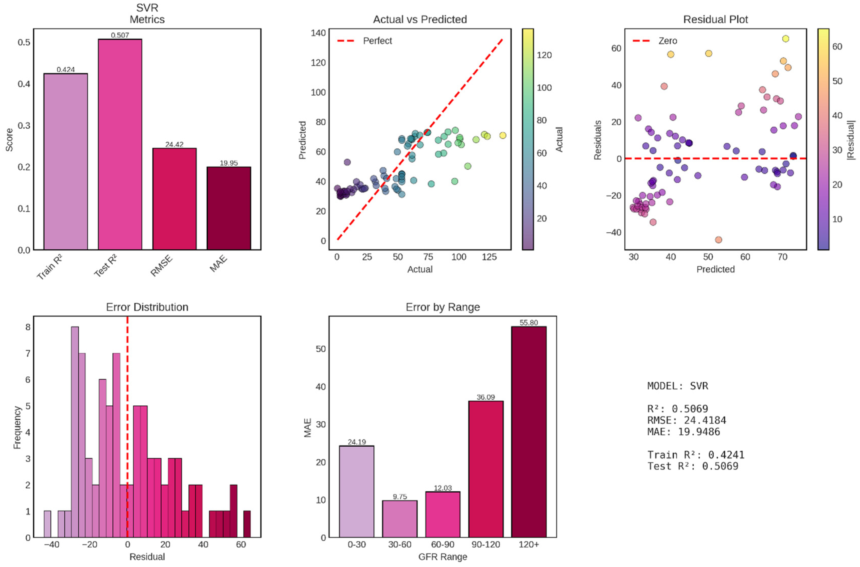
Support Vector Regression (SVR) with radial basis function (RBF) kernel achieved poor performance for continuous GFR prediction, with a test R2 of 0.507 explaining only 50.7% of variance—essentially equivalent to Ridge regression (51.4%) and dramatically inferior to Random Forest (91.4%). The model’s test RMSE of 24.42 mL/min/1.73m2 and MAE of 19.95 mL/min/1.73m2 are virtually identical to Ridge regression’s errors (RMSE 24.25, MAE 18.89), suggesting that despite SVR’s theoretical capacity for non-linear modeling through kernel functions, it failed to capture complex patterns beyond what simple linear regression achieved shown in Figure 11. Most concerning, the model exhibits systematic bias, severe heteroscedasticity, and catastrophically poor performance at high GFR values, rendering it clinically unsuitable for deployment.
The test R2 of 0.507 represents disappointingly modest performance, explaining barely half of GFR variance and performing 44 percentage points worse than Random Forest. Perhaps more unusual is the training R2 of only 0.424—worse than test performance by 8.3 percentage points. This negative train-test gap (where test performance exceeds training performance) is highly atypical and suggests fundamental problems with model fitting or hyperparameter configuration. The test RMSE of 24.42 mL/min/1.73m2 is virtually identical to Ridge regression’s 24.25, representing no improvement despite SVR’s theoretical advantages in handling non-linear relationships through kernel transformations. Similarly, the MAE of 19.95 mL/min/1.73m2 closely matches Ridge’s 18.89, indicating that typical prediction errors span approximately 20 mL/min/1.73m2—sufficient to cause frequent CKD stage misclassifications and undermine clinical utility.
The RMSE-MAE gap of 4.47 mL/min/1.73m2 (RMSE 24.42 vs MAE 19.95) is actually smaller than Ridge’s gap of 5.36, suggesting proportionally fewer extreme outliers in SVR predictions. However, this apparent advantage is illusory, as the actual vs predicted plot reveals that SVR achieves lower outlier frequency by systematically compressing predictions into a narrow range (approximately 30-70 mL/min/1.73m2), thereby avoiding extreme errors but also failing to capture the full GFR spectrum. This compression represents a fundamental failure mode where the model “plays it safe” by predicting near-average values rather than attempting to discriminate across the full physiological range.
4. Conclusion
This study systematically evaluated machine learning algorithms for chronic kidney disease classification and GFR prediction using clinical and laboratory data from 400 patients. For binary CKD classification, Logistic Regression and Random Forest both achieved exceptional 98.75% test accuracy, with Logistic Regression offering superior interpretability and Random Forest demonstrating better cross-validation stability (CV ± 0.99% vs ± 1.59%). Gradient Boosting achieved 96.25% accuracy on a three-class problem, though with concerning false negatives where CKD patients were completely missed.
For continuous GFR prediction, Random Forest substantially outperformed all competitors with test R2 of 0.914, RMSE of 10.20 mL/min/1.73m2, and MAE of 4.37 mL/min/1.73m2, representing clinically meaningful precision suitable for staging, medication dosing, and treatment planning decisions. The model demonstrated homoscedastic residuals and consistent accuracy across the full GFR spectrum (MAE ranging only from 1.36 to 8.84 across different ranges). In contrast, Ridge Regression achieved modest performance (R2 = 0.514, MAE = 18.89) with severe heteroscedasticity and range-dependent accuracy, while Support Vector Regression performed poorly (R2 = 0.507, MAE = 19.95) with catastrophic errors at high GFR values (MAE = 55.80 for GFR >120) and systematic prediction compression.
The results establish Random Forest as the optimal approach for both CKD classification and GFR prediction tasks, combining near-perfect diagnostic accuracy with precise quantitative GFR estimation that substantially exceeds standard clinical equations. The model’s ability to capture non-linear relationships and feature interactions without manual specification, coupled with built-in regularization through ensemble averaging, enables robust performance across diverse patient presentations. However, clinical deployment requires addressing interpretability limitations through explainability tools, validating performance on external populations, and implementing confidence intervals to communicate prediction uncertainty. Future work should focus on external validation across different healthcare settings, integration with electronic health record systems, and prospective evaluation of clinical impact on patient outcomes and healthcare utilization.
References
- Vivante, A., 2024. Genetics of chronic kidney disease. New England Journal of Medicine, 391(7), pp.627-639.
- Francis, A.; Harhay, M.N.; Ong, A.C.M.; Tummalapalli, S.L.; Ortiz, A.; Fogo, A.B.; Fliser, D.; Roy-Chaudhury, P.; Fontana, M.; Nangaku, M.; et al. Chronic kidney disease and the global public health agenda: an international consensus. Nat. Rev. Nephrol. 2024, 20, 473–485. [CrossRef]
- EMPA-KIDNEY Collaborative Group, 2025. Long-term effects of empagliflozin in patients with chronic kidney disease. New England Journal of Medicine, 392(8), pp.777-787.
- Jadoul, M.; Aoun, M.; Imani, M.M. The major global burden of chronic kidney disease. Lancet Glob. Heal. 2024, 12, e342–e343. [CrossRef]
- Stevens, P.E., Ahmed, S.B., Carrero, J.J., Foster, B., Francis, A., Hall, R.K., Herrington, W.G., Hill, G., Inker, L.A., Kazancıoğlu, R. and Lamb, E., 2024. KDIGO 2024 clinical practice guideline for the evaluation and management of chronic kidney disease. Kidney international, 105(4), pp.S117-S314.
- Miguel, V.; Shaw, I.W.; Kramann, R. Metabolism at the crossroads of inflammation and fibrosis in chronic kidney disease. Nat. Rev. Nephrol. 2024, 21, 39–56. [CrossRef]
- Hasan, H., Rahman, M.H., Haque, M.A., Rahman, M.S., Ali, M.S. and Sultana, S., 2024. Nutritional management in patients with chronic kidney disease: A focus on renal diet. Asia Pacific Journal of Medical Innovations, 1(1), pp.34-40.
- Vazquez, M.A.; Oliver, G.; Amarasingham, R.; Sundaram, V.; Chan, K.; Ahn, C.; Zhang, S.; Bickel, P.; Parikh, S.M.; Wells, B.; et al. Pragmatic Trial of Hospitalization Rate in Chronic Kidney Disease. New Engl. J. Med. 2024, 390, 1196–1206. [CrossRef]
- Delrue, C.; De Bruyne, S.; Speeckaert, M.M. Application of Machine Learning in Chronic Kidney Disease: Current Status and Future Prospects. Biomedicines 2024, 12, 568. [CrossRef]
- Khalid, F.; Alsadoun, L.; Khilji, F.; Mushtaq, M.; Eze-Odurukwe, A.; Mushtaq, M.M.; Ali, H.; Farman, R.O.; Ali, S.M.; Fatima, R.; et al. Predicting the Progression of Chronic Kidney Disease: A Systematic Review of Artificial Intelligence and Machine Learning Approaches. Cureus 2024, 16, e60145. [CrossRef]
- Gogoi, P.; Valan, J.A. Machine learning approaches for predicting and diagnosing chronic kidney disease: current trends, challenges, solutions, and future directions. Int. Urol. Nephrol. 2024, 57, 1245–1268. [CrossRef]
- Rahman, M.; Amin, A.; Hossain, J. Machine learning models for chronic kidney disease diagnosis and prediction. Biomed. Signal Process. Control. 2023, 87. [CrossRef]
- Dutta, S., Sikder, R., Islam, M.R., Al Mukaddim, A., Hider, M.A. and Nasiruddin, M., 2024. Comparing the Effectiveness of Machine Learning Algorithms in Early Chronic Kidney Disease Detection. Journal of Computer Science and Technology Studies, 6(4), pp.77-91.
- Ghosh, B.P.; Imam, T.; Anjum, N.; Mia, T.; Siddiqua, C.U.; Sharif, K.S.; Khan, M.; Mamun, A.I.; Hossain, Z. Advancing Chronic Kidney Disease Prediction: Comparative Analysis of Machine Learning Algorithms and a Hybrid Model. J. Comput. Sci. Technol. Stud. 2024, 6, 15–21. [CrossRef]
- Ghosh, S.K.; Khandoker, A.H. Investigation on explainable machine learning models to predict chronic kidney diseases. Sci. Rep. 2024, 14, 1–15. [CrossRef]
- Arif, M.S.; Rehman, A.U.; Asif, D. Explainable Machine Learning Model for Chronic Kidney Disease Prediction. Algorithms 2024, 17, 443. [CrossRef]
- Rahat, A.R.; Islam, T.; Cao, D.M.; Tayaba, M.; Ghosh, B.P.; Ayon, E.H.; Nobe, N.; Akter, A.; Rahman, M.; Bhuiyan, M.S.; et al. Comparing Machine Learning Techniques for Detecting Chronic Kidney Disease in Early Stage. J. Comput. Sci. Technol. Stud. 2024, 6, 20–32. [CrossRef]
- Ekundayo, F. Machine learning for chronic kidney disease progression modelling: Leveraging data science to optimize patient management. World J. Adv. Res. Rev. 2024, 24, 453–475. [CrossRef]
Figure 1.
Workflow diagram for machine learning-based chronic kidney disease classification and GFR prediction. The analytical pipeline comprises four main stages: (1) Data source: CKD dataset containing demographic variables (age), vital signs (blood pressure), urinalysis parameters (specific gravity, albumin, sugar, red blood cells, pus cells, pus cell clumps, bacteria), and hematological indices (hemoglobin, packed cell volume, white blood cell count, red blood cell count, appetite); (2) Preprocessing: systematic handling of missing values through mode/median imputation, label encoding of categorical variables, and feature standardization using z-score normalization; (3) Modeling: parallel implementation of classification algorithms (Logistic Regression, Random Forest, Gradient Boosting, Support Vector Machine) and regression algorithms (Linear Regression, Ridge Regression, Lasso Regression, Random Forest Regressor, Gradient Boosting Regressor, Support Vector Regression) for CKD detection and GFR prediction, respectively; (4) Evaluation: comprehensive performance assessment using classification metrics (accuracy, precision, recall, F1-score, confusion matrices) for categorical outcomes and regression metrics (R2, RMSE, MAE, residual analysis) for continuous GFR predictions. The bidirectional workflow allows simultaneous optimization of both classification and regression objectives using identical preprocessed features.
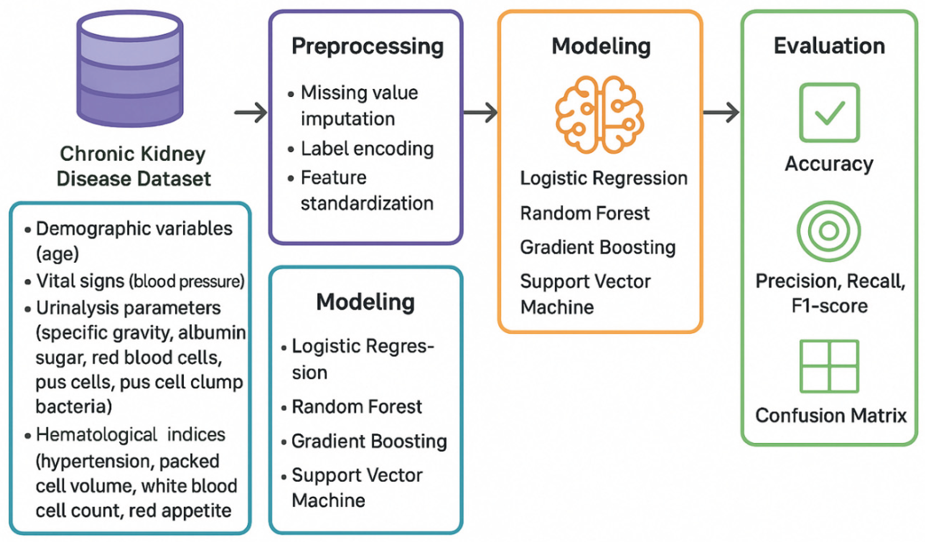
Figure 3.
Distribution of Glomerular Filtration Rate (GFR) Values in the Study Population. The histogram displays the frequency distribution of GFR values (mL/min/1.73m2) across the dataset, with a gradient color scheme transitioning from dark blue (lower GFR values) to yellow-green (higher GFR values) representing the progression from severe to mild kidney function. The red dashed line indicates the mean GFR (56.59 mL/min/1.73m2), while the orange dashed line marks the median GFR (53.28 mL/min/1.73m2). The distribution exhibits a bimodal pattern with peaks in the severely reduced GFR range (0-10 mL/min/1.73m2) and the moderately reduced range (60-70 mL/min/1.73m2), reflecting the heterogeneous spectrum of kidney function in the study cohort.
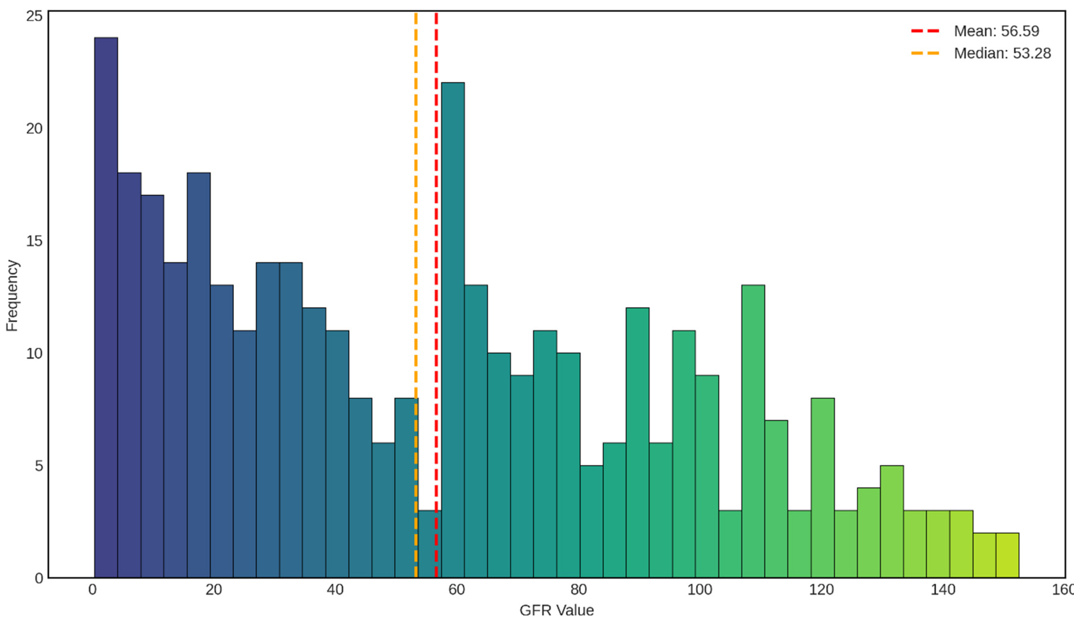
Figure 4.
Distribution of Chronic Kidney Disease (CKD) Stages in the Study Cohort. The bar chart illustrates the frequency distribution of patients across six CKD stages (Stage 0 through Stage 5), with color coding transitioning from green (Stage 0, no CKD or normal kidney function) through yellow-orange (intermediate stages) to red (Stage 5, kidney failure). Stage 0 represents individuals without CKD (n=89), Stage 1 indicates kidney damage with normal or high GFR ≥90 mL/min/1.73m2 (n=78), Stage 2 represents mild reduction in GFR 60-89 mL/min/1.73m2 (n=34), Stage 3 indicates moderate reduction in GFR 30-59 mL/min/1.73m2 (n=45), Stage 4 represents severe reduction in GFR 15-29 mL/min/1.73m2 (n=58), and Stage 5 indicates kidney failure with GFR <15 mL/min/1.73m2 or dialysis requirement (n=96). The distribution demonstrates a U-shaped pattern with the highest frequencies at both extremes of the disease spectrum.
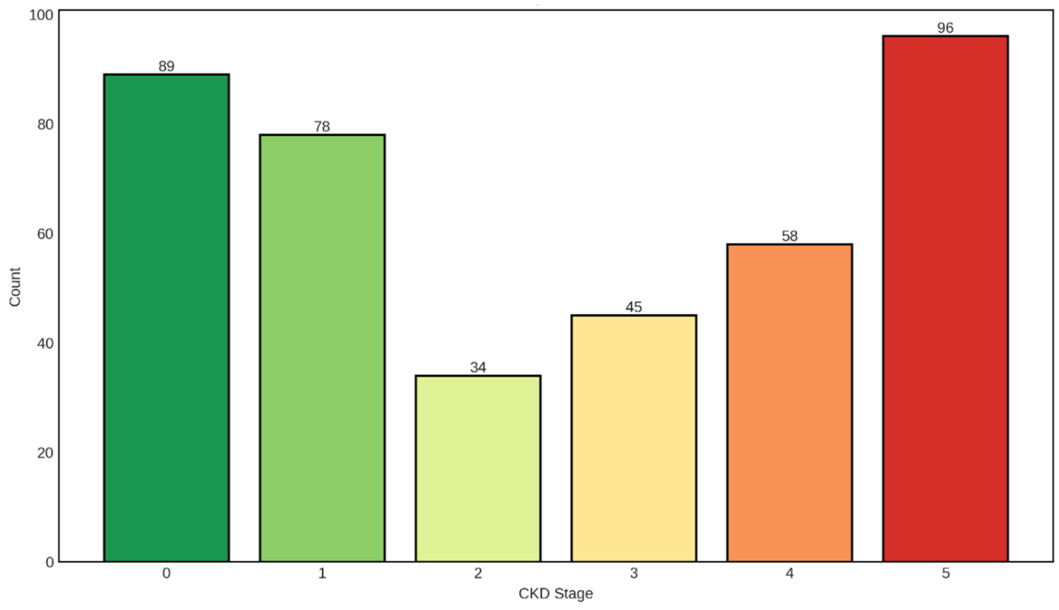
Figure 5.
Feature Correlation Heatmap of Clinical and Laboratory Parameters. The heatmap displays Pearson correlation coefficients between 24 clinical and laboratory features in the CKD dataset. The color gradient ranges from dark blue (strong negative correlation, r ≈ -0.6) through white (no correlation, r ≈ 0) to dark red (strong positive correlation, r ≈ 1.0). Features are arranged along both axes and include: age, blood pressure (bp), specific gravity (sg), albumin (al), sugar (su), red blood cells (rbc), pus cells (pc), pus cell clumps (pcc), bacteria (ba), blood glucose random (bgr), blood urea (bu), serum creatinine (sc), sodium (sod), potassium (pot), hemoglobin (hemo), packed cell volume (pcv), white blood cell count (wc), red blood cell count (rc), hypertension (htn), diabetes mellitus (dm), coronary artery disease (cad), appetite (appet), pedal edema (pe), and anemia (ane). The diagonal shows perfect self-correlation (r = 1.0), while off-diagonal elements reveal inter-feature relationships relevant for feature selection and multicollinearity assessment.
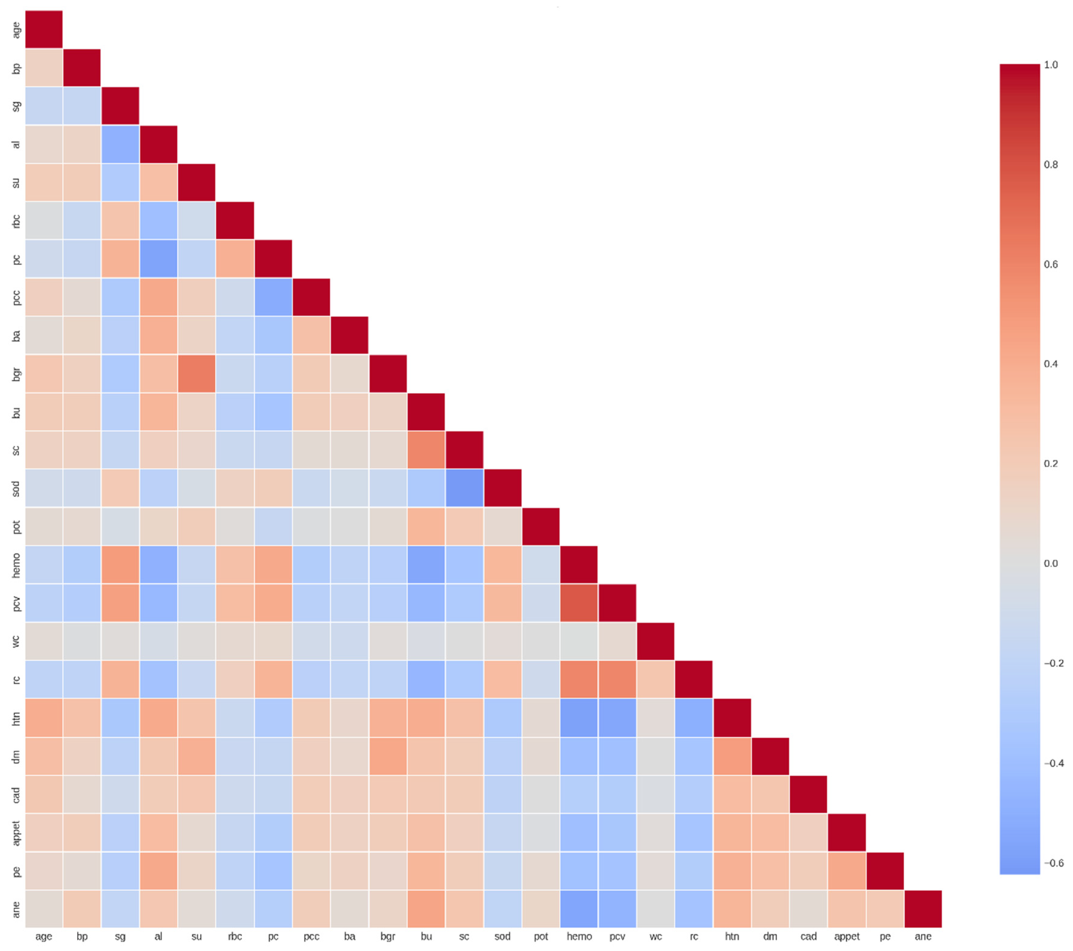
Figure 6.
Performance Evaluation of Logistic Regression Model for CKD Classification. The figure comprises six panels presenting comprehensive performance metrics for the logistic regression classifier. Top left: Performance metrics showing training accuracy (0.997), test accuracy (0.988), precision (0.988), recall (0.988), and F1-score (0.988). Top middle: Cross-validation (CV) score demonstrating robust model generalization (0.978 ± 0.016). Top right: Confusion matrix on the test set displaying true negatives (49), false positives (1), false negatives (0), and true positives (30), indicating excellent discriminative ability. Bottom left: Comparison of training versus test accuracy (0.997 vs 0.988) showing minimal overfitting with a train-test gap of 0.009. Bottom middle: Detailed breakdown of precision (0.988), recall (0.988), and F1-score (0.988). Bottom right: Summary statistics confirming the model’s strong predictive performance across all evaluation metrics.
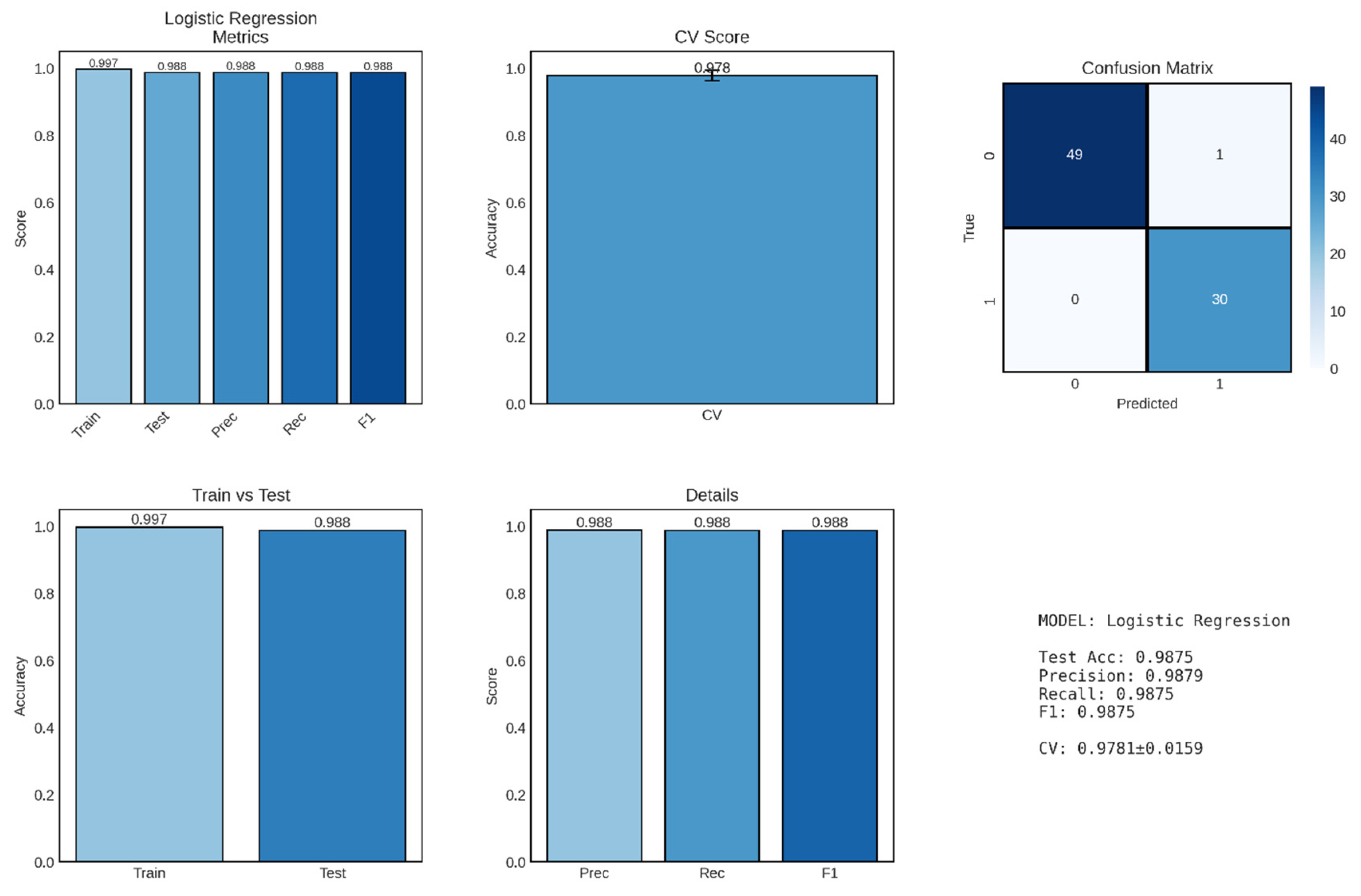
Figure 7.
Performance Evaluation of Random Forest Model for CKD Classification. The figure presents comprehensive performance metrics for the Random Forest ensemble classifier across six panels. Top left: Performance metrics displaying perfect training accuracy (1.000), test accuracy (0.988), precision (0.988), recall (0.988), and F1-score (0.987). Top middle: Cross-validation (CV) score demonstrating exceptional model stability (0.984 ± 0.010). Top right: Confusion matrix on the test set showing true negatives (50), false positives (0), false negatives (1), and true positives (29), indicating near-perfect classification with only one misclassification. Bottom left: Comparison of training versus test accuracy (1.000 vs 0.988) revealing minimal overfitting with a train-test gap of 1.2%. Bottom middle: Detailed breakdown of precision (0.988), recall (0.988), and F1-score (0.987). Bottom right: Summary statistics confirming the model’s robust predictive performance with the lowest cross-validation variability among all classifiers tested.
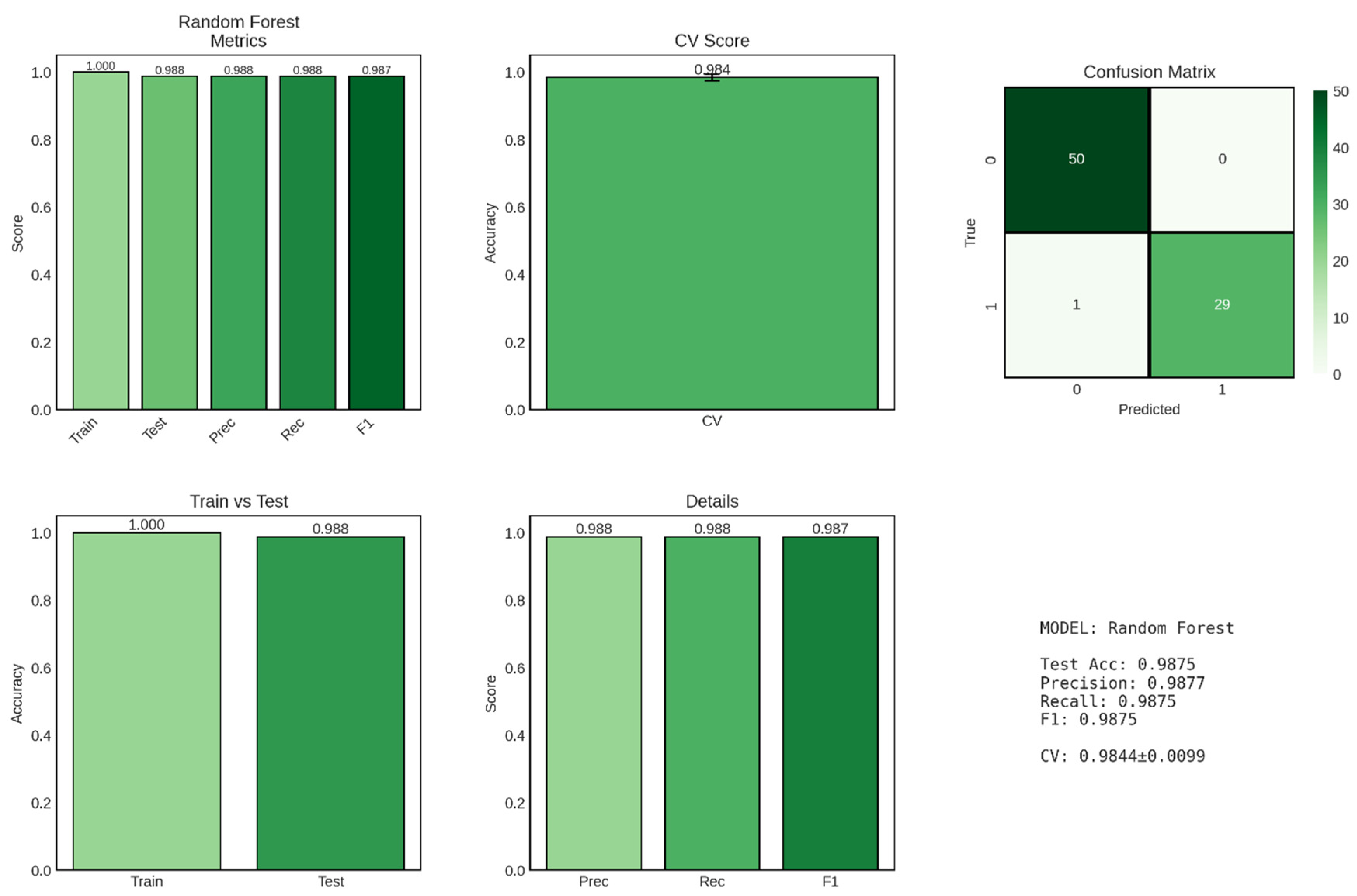
Figure 8.
Performance Evaluation of Gradient Boosting Model for CKD Classification. The figure displays comprehensive performance metrics for the Gradient Boosting classifier across six panels, with predictions across three classes (0, 1, 2). Top left: Performance metrics showing perfect training accuracy (1.000), test accuracy (0.963), precision (0.975), recall (0.963), and F1-score (0.969). Top middle: Cross-validation (CV) score demonstrating strong model stability (0.956 ± 0.021). Top right: Confusion matrix on the test set displaying predictions for three classes, with 49 correct predictions for class 0, 1 misclassification between class 0 and class 1, 28 correct predictions for class 2, and 2 misclassifications from class 2 to class 0, totaling 3 errors out of 80 test cases (96.25% accuracy). Bottom left: Comparison of training versus test accuracy (1.000 vs 0.963) showing a train-test gap of 3.7%. Bottom middle: Detailed breakdown of precision (0.975), recall (0.963), and F1-score (0.969). Bottom right: Summary statistics confirming robust multi-class classification performance.
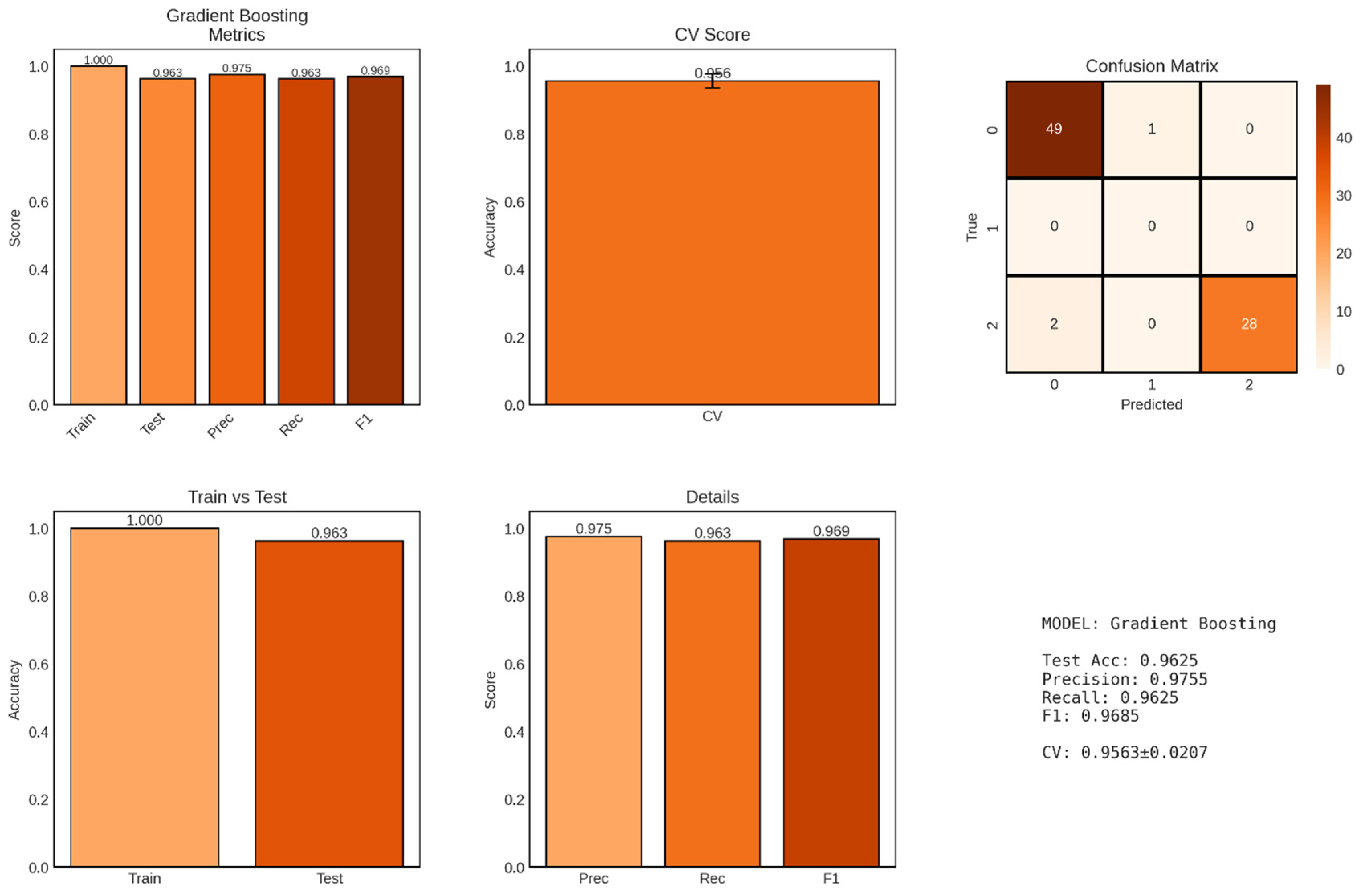
Figure 9.
Performance Evaluation of Ridge Regression Model for GFR Prediction. The figure comprises six panels presenting comprehensive metrics for the Ridge regression model. Top left: Performance metrics showing training R2 (0.686), test R2 (0.514), RMSE (24.25), and MAE (18.89). Top middle: Actual vs Predicted GFR scatter plot with points color-coded by actual GFR values, demonstrating moderate correlation with the perfect prediction line (red dashed) and notable scatter, particularly at extreme GFR values. Top right: Residual plot showing prediction errors versus predicted values, with residuals color-coded by magnitude and scattered around the zero line (red dashed), revealing heteroscedasticity with larger errors at higher predicted GFR values. Bottom left: Error distribution histogram showing approximately normal distribution of residuals centered near zero (red dashed line) with some outliers. Bottom middle: Mean Absolute Error stratified by GFR ranges (0-30, 30-60, 60-90, 90-120, 120+ mL/min/1.73m2), showing increasing prediction error with higher GFR values (MAE ranging from 15.54 to 30.96). Bottom right: Summary statistics confirming moderate predictive performance with substantial train-test R2 gap (0.172) indicating overfitting.
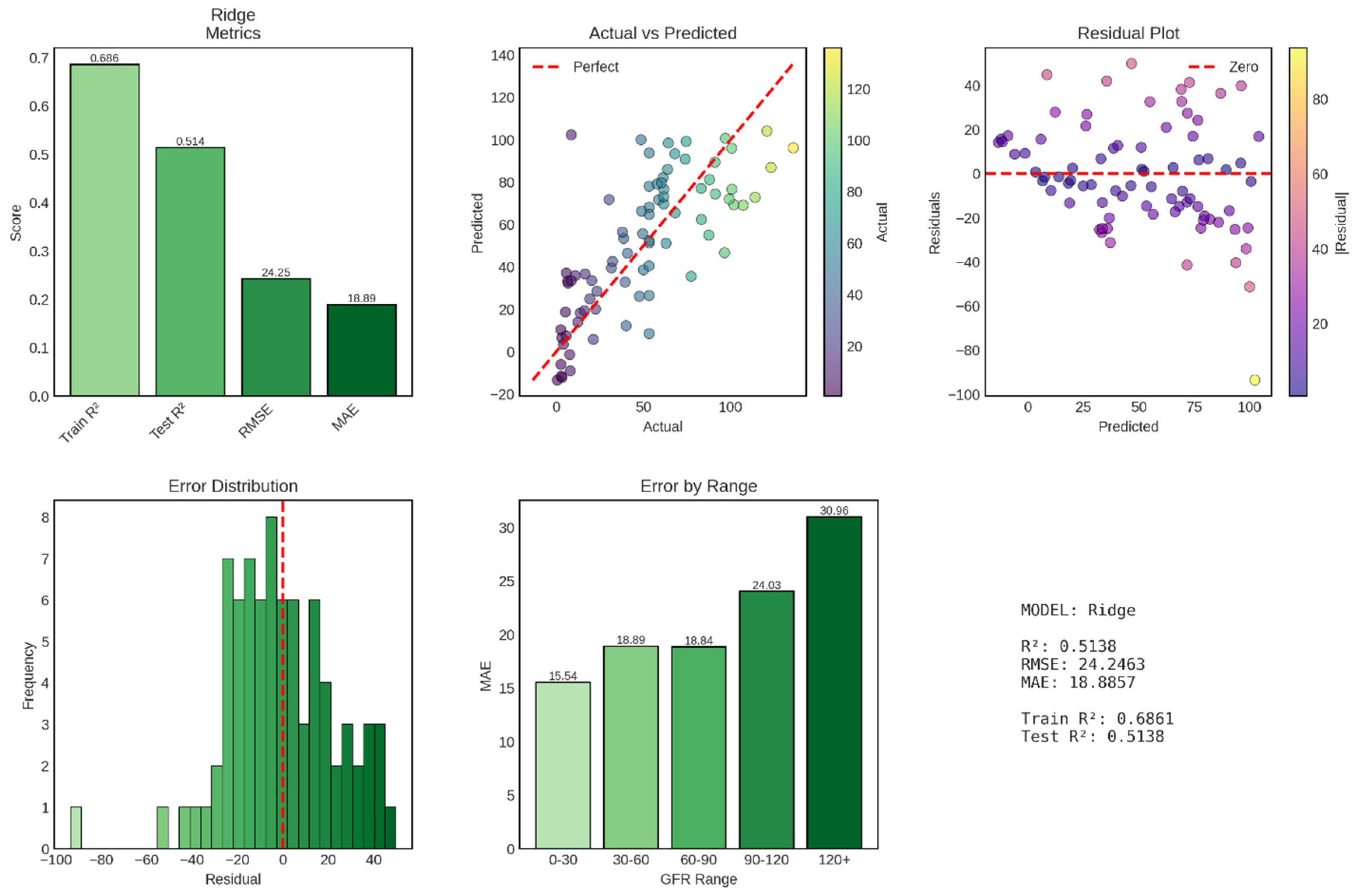
Figure 10.
Performance Evaluation of Random Forest Regression Model for GFR Prediction. The figure presents comprehensive metrics for the Random Forest regression model across six panels. Top left: Performance metrics displaying training R2 (0.997), test R2 (0.914), RMSE (10.20), and MAE (4.37). Top middle: Actual vs Predicted GFR scatter plot with points color-coded by actual GFR values, showing strong correlation with the perfect prediction line (red dashed) and minimal scatter across the entire GFR range. Top right: Residual plot showing prediction errors versus predicted values, with residuals tightly clustered around the zero line (red dashed), indicating homoscedastic errors and unbiased predictions. Bottom left: Error distribution histogram displaying approximately normal distribution of residuals centered at zero with narrow spread (most errors between -10 and +10 mL/min/1.73m2). Bottom middle: Mean Absolute Error stratified by GFR ranges showing remarkably consistent performance across the spectrum, with lowest error in the 60-90 range (MAE = 1.36) and highest in the 30-60 range (MAE = 8.84). Bottom right: Summary statistics confirming excellent predictive performance with minimal overfitting (train-test R2 gap of 8.3%).
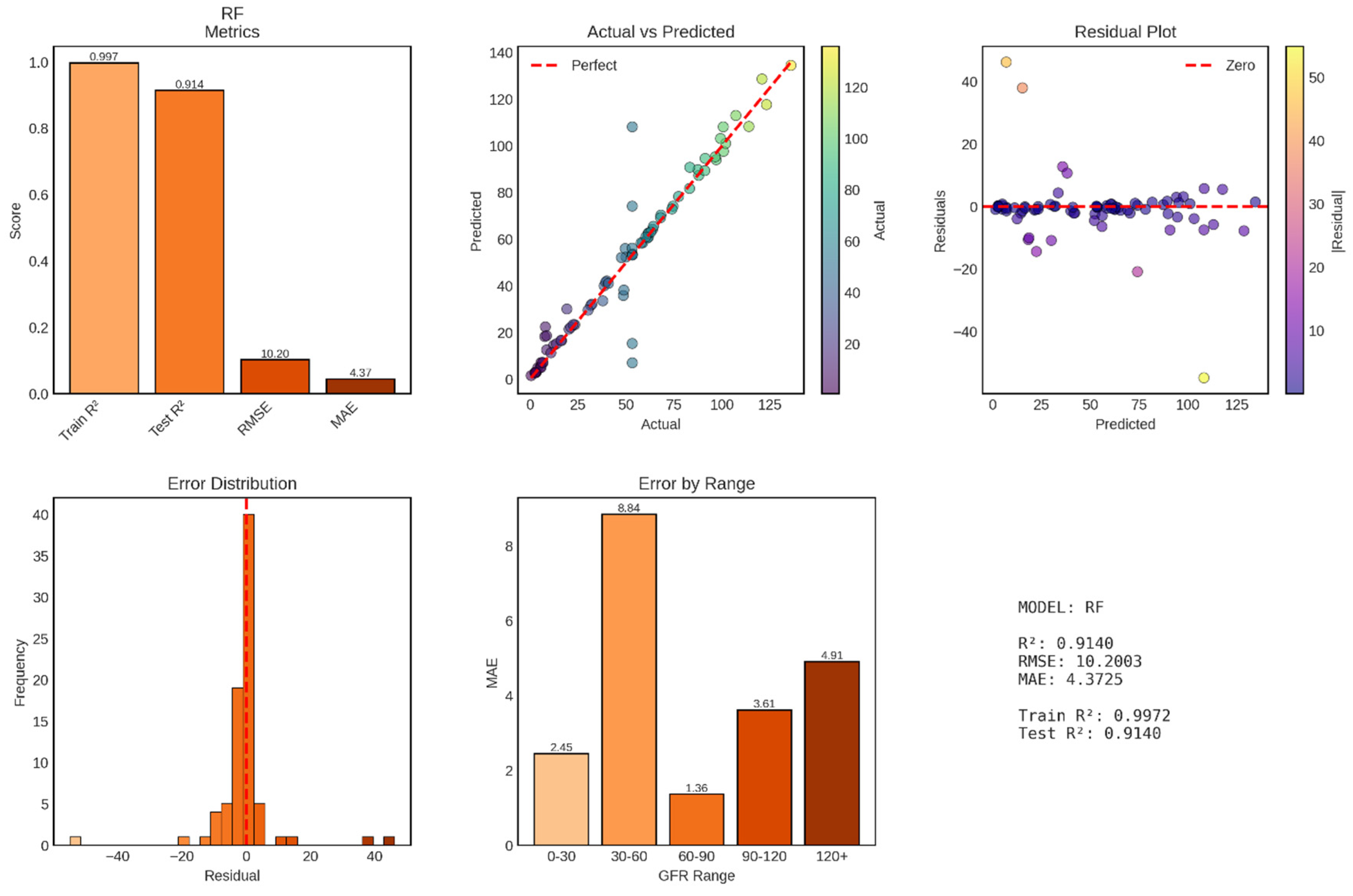
Figure 11.
Performance Evaluation of Support Vector Regression (SVR) Model for GFR Prediction. The figure displays comprehensive metrics for the SVR model across six panels. Top left: Performance metrics showing training R2 (0.424), test R2 (0.507), RMSE (24.42), and MAE (19.95). Top middle: Actual vs Predicted GFR scatter plot with points color-coded by actual GFR values, revealing substantial scatter and systematic underprediction at high GFR values with predictions compressed in the 30-70 mL/min/1.73m2 range. Top right: Residual plot showing heteroscedastic errors with increasing variance at higher predicted values and systematic positive bias (underprediction) for high actual GFR cases. Bottom left: Error distribution histogram displaying non-normal, left-skewed distribution centered slightly below zero, indicating systematic underprediction bias. Bottom middle: Mean Absolute Error stratified by GFR ranges showing dramatic performance variation, with best accuracy in the 30-60 range (MAE = 9.75) and catastrophically poor performance in the 120+ range (MAE = 55.80). Bottom right: Summary statistics confirming poor overall performance with negative train-test R2 gap (-8.3%), indicating worse training than test performance.
Disclaimer/Publisher’s Note: The statements, opinions and data contained in all publications are solely those of the individual author(s) and contributor(s) and not of MDPI and/or the editor(s). MDPI and/or the editor(s) disclaim responsibility for any injury to people or property resulting from any ideas, methods, instructions or products referred to in the content. |
© 2026 by the authors. Licensee MDPI, Basel, Switzerland. This article is an open access article distributed under the terms and conditions of the Creative Commons Attribution (CC BY) license.
Copyright: This open access article is published under a Creative Commons CC BY 4.0 license, which permit the free download, distribution, and reuse, provided that the author and preprint are cited in any reuse.


