1. Introduction
The kidneys are vital in filtering excess water and waste from the bloodstream to produce urine. Elevated blood glucose levels, characteristic of diabetes, can impair the blood vessels within the kidneys, diminishing their functionality. Classified as a microvascular consequence, Diabetic Kidney Disease (DKD) can appear in patients with type 1 diabetes (T1DM) or type 2 diabetes (T2DM). Kidney failure may result from DKD because the kidney’s microscopic blood capillaries are damaged by high blood glucose levels, which lessens the kidney’s capacity to filter waste and extra water. Diabetic kidney disease or diabetic nephropathy, is a common complication arising from diabetes, affecting roughly one-third of adults with the condition. Its occurrence is more pronounced in individuals aged 65 years or older, with 38% affected, compared to those aged between 45 to 64 years (13%) or between 18 to 44 years (7%) [
1]. Diabetes-related death rates increased by 3% between 2000 and 2019, with lower-middle-income countries experiencing a notable 13% increase in these rates [
2]. Notably, adults afflicted with DKD face a heightened risk of premature mortality compared to their counterparts without DKD of similar age.
Predicting diabetic kidney disease (DKD) involves a comprehensive approach using clinical assessments and lab tests like serum creatinine, eGFR, and urine ACR. Monitoring blood pressure and glycemic control is vital, as hypertension and poor blood sugar management are DKD risk factors. Genetic testing can identify predispositions, while imaging studies provide insights into kidney structure. Risk prediction models incorporating demographic, medical, and lab data estimate DKD risk. Biomarkers such as KIM-1 and suPAR show promise in predicting DKD progression. Regular clinical assessments are crucial for early detection and intervention. The conventional upper limit for urine albumin is 30 mg/day, with values >300 mg/day termed macroalbuminuria and those between 30-300 mg/day traditionally called microalbuminuria [
3]. Macroalbuminuria and microalbuminuria serve as key indicators in identifying and monitoring DKD, reflecting kidney damage in individuals with diabetes and aiding clinicians in assessing the progression and severity of the disease.
Current methods for predicting Diabetic Kidney Disease (DKD) rely on assessing causative factors such as blood pressure, blood glucose levels, and kidney function tests. However, these methods often fall short in accurately predicting DKD due to their reliance on a limited set of indicators and static models that do not adapt over time. Manual analysis further complicates the process, leading to variability in diagnosis and treatment decisions. Machine learning (ML) offers a transformative solution by leveraging large volumes of clinical data to identify intricate patterns and associations that may be missed by conventional methods. ML algorithms excel in feature selection and engineering, capturing complex relationships between variables and dynamically updating models to reflect changes in patient health status. By automating analysis and generating personalized risk assessments, ML facilitates timely intervention. With its scalability and potential for widespread adoption, ML holds promise in revolutionizing DKD prediction, empowering healthcare providers to manage better and mitigate the impact of this debilitating condition.
This paper presents a comparative analysis of machine learning algorithms such as Logistic Regression (LR), Decision Tree (DT), Random Forest (RF), Bayesian Tree Model (BTM), and Support Vector Machine (SVM) for determining the effective model for predicting Diabetic Kidney Disease. The main contributions of this study are as follows:
XGBoost along with SHAP(SHapley Additive exPlanations) was employed for feature selection to enhance the model performance and decrease overfitting.
The well known machine learning classification algorithms such as Logistic Regression (LR), Decision Tree (DT), Random Forest (RF), Bayesian Tree Model (BTM), and Support Vector Machine (SVM) were trained and evaluated using performance evaluation metrics such as Accuracy, Precision, Recall, Specificity, F1-score and AUC for their effectiveness in predicting kidney disease.
Most common Swarm Intelligence-based algorithms were utilized for optimization of hyperparameters. Specifically, Particle Swarm Optimization was applied to XGBoost, while Firefly Optimization(FFO) and Ant Colony Optimization(ACO) were utilized for optimizing the LR, DT, RF, BTM and SVM machine learning models. The performance of all models before and after applying FFO and ACO optimization algorithms were compared based on the evaluation metrics.
The performance of the models was trained and evaluated using a clinical report dataset, which includes diverse information about diabetic patients collected from a private hospital in Coimbatore.
The paper’s structure is as follows:
Section 2 presents a review of related research concerning the prediction of Chronic Kidney Disease utilizing multiple classifiers.
Section 3 details the methodology employed in our study, encompassing data collection, preprocessing, feature selection, dataset splitting, and the development of models utilizing various machine learning algorithms. In
Section 4, the results and discussions of our work are presented. Finally,
Section 5 concludes our findings and discusses future plans.
2. Related Work
In 2015, Vijayarani and Dhayanand [
4] compared Naïve Bayes and Support Vector Machine (SVM) using a synthetic kidney function test (KFT) dataset. Their findings indicated that while SVM achieved higher accuracy (76.32%), Naïve Bayes exhibited faster execution times. This study underscored the conflicts between accuracy and computational efficiency and emphasized the importance of data preprocessing. In 2017, Gunarathne et al. [
5] employed various machine learning classification algorithms to predict the status of chronic kidney disease (CKD) using a dataset with 400 instances and 25 variables from the UCI repository. Among the algorithms tested, the Multiclass Decision Forest achieved the highest accuracy of 99.1% using only 14 attributes, outperforming other models that used more attributes. This finding demonstrated that fewer attributes could lead to higher accuracy and faster predictions, which is crucial for early treatment initiation. However, the study also pointed out limitations, including a small dataset size and missing attribute values, indicating a need for larger datasets with complete records for further improvement. Both studies illustrate the potential and challenges of using machine learning in predicting kidney disease, emphasizing the need for balancing accuracy and computational efficiency, as well as the importance of comprehensive and robust datasets.
In 2018, Siddheshwar Tekale et al. [
6] further explored the UCI CKD dataset using Decision Tree and SVM, achieving accuracies of 91.75% and 96.75%, respectively. This reinforced the superior performance of SVM noted by Vijayarani and Dhayanand[
4], while also highlighting the necessity for larger datasets with complete records for robust predictions. Building on this, Revathy et al. [
7] in 2019 evaluated Decision Trees, SVM, and Random Forest, with Random Forest achieving the highest accuracy of 99.16%. This demonstrated the potential of advanced algorithms for more accurate CKD prediction, a trend continued in later studies.
Jyoti Rani’s [
8] study in 2020 explored advanced machine learning applications by employing Decision Tree, Random Forest, Gradient Boosting, and K-Nearest Neighbors, utilizing Ant Colony Optimization for feature selection. Both Random Forest and Gradient Boosted Trees performed exceptionally well, particularly in predicting diabetic kidney disease (DKD) within five years of T2DM diagnosis. This study addressed the limitations of earlier works regarding dataset size and missing data handling, highlighting the importance of feature selection techniques and large datasets.
In 2021, Gazi et al. [
9] examined various machine learning models, including Decision Tree, Random Forest, SVM, K-Nearest Neighbors, and Naive Bayes. Random Forest again achieved the highest accuracy at 99%, reaffirming its robust prediction capabilities as observed by Revathy et al.[
7] This study emphasized model selection based on specific criteria, noting that computational complexity and overfitting remain challenges, consistent with findings by Jyoti Rani [
8]. Angier Allen et al. [
10] in 2022 focused on predicting DKD within five years of an initial T2DM diagnosis using machine learning algorithms and electronic health records (EHRs). Random Forest and Gradient Boosted Trees (XGB) were compared to the CDC risk score. This study leveraged readily accessible EHR data without requiring urinary albumin measurements, facilitating broader screening for DKD and echoing the effectiveness of Random Forest observed in previous studies.
In 2023 [
11], Pal performed a study aimed at early detection of CKD utilized machine learning algorithms, including SVM, Random Forest, and Artificial Neural Network classifiers, applied to a UCI dataset. Random Forest emerged as the best performer with an accuracy of 0.92, benefiting from a combination of categorical and non-categorical attributes. However, limitations included the relatively small dataset size and lack of feature selection methods, issues addressed through advanced techniques like those used by Jyoti Rani[
8]. Additionally, Chamandeep Kaur et al. [
12] explored various machine learning models, including Decision Trees, Random Forests, and Gradient Boosted Trees, using Ant Colony Optimization for feature selection. RF and XGB showed high accuracy, with RF yielding an AUROC of 0.930 for CKD prediction. This study demonstrated significant potential for early disease detection, although improvements in handling missing data and overfitting were needed, consistent challenges identified in previous research.
Overall, the existing studies collectively contribute to advancing DKD prediction by addressing various limitations and refining methodologies to enhance predictive accuracy and efficiency. The common research gaps identified from the literature review include:
Small dataset sizes and challenges in handling missing data.
Potential biases in the training data was not discussed.
Unclear data description
Information about the generalizability of the proposed predictive models for diabetic kidney disease to different populations or settings was not provided.
Apart from few of the existing studies, mostly the importance of feature selection and model optimization remains unaddressed. The recurring use of advanced algorithms, such as SVM, Random Forest, and Gradient Boosted Trees, along with sophisticated feature selection techniques, underscores the ongoing efforts to mitigate these issues.
The proposed system addressed these limitations by deeply analyzing and utilizing an augmented dataset that includes clinical data for training the model. In addition to this, feature selection and Swarm Intelligence based optimization techniques were used for enhancing the performance of the machine learning models.
3. Methodology
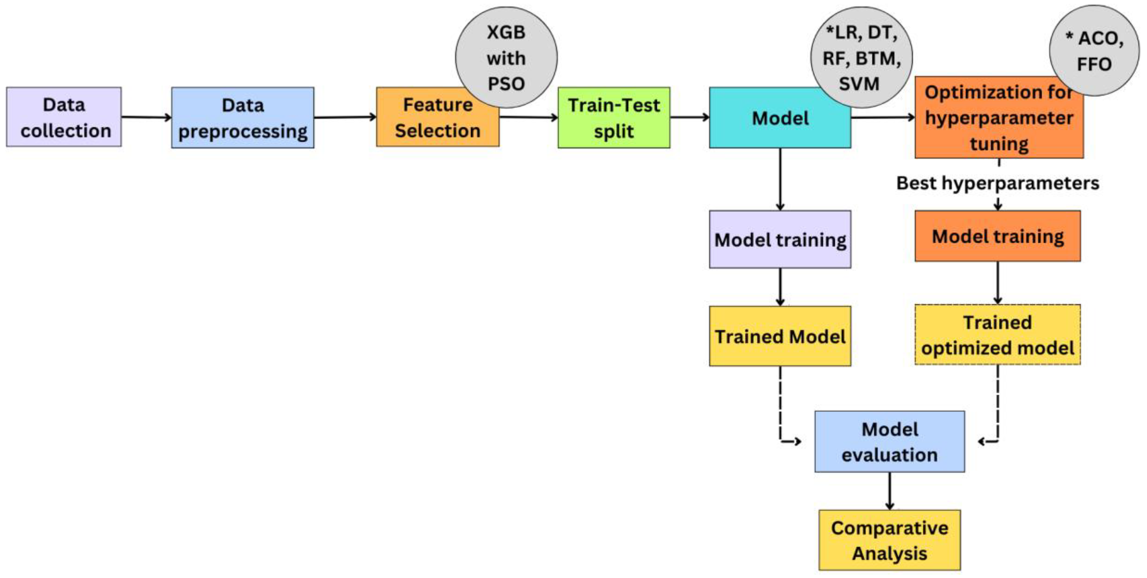
This research study performs a comparative analysis of machine learning models such as Logistic Regression (LR), Decision Tree (DT), Random Forest (RF), Bayesian Tree Model (BTM), and Support Vector Machine (SVM) for determining the robust model for predicting Diabetic Kidney Disease. The proposed methodology for predicting Chronic Kidney Disease (DKD) begins with data collection and preprocessing, followed by splitting the data into train and test datasets. Feature extraction is carried out on the dataset using XGBoost combined with Particle Swarm Optimization (PSO). This process involves training the XGBoost model and optimizing it with PSO to determine the attributes that contribute to the highest accuracy. These selected features are then used to train and test ML models such as LR, DT, RF, BTM, and SVM. The models are initially evaluated using these features, and the results are recorded. The machine learning models are then further optimized by tuning the hyperparameters using Ant Colony Optimization(ACO) and Firefly Optimization(FFO) techniques. The optimized models are re-evaluated, and their performance metrics are tabulated. Finally, a comparative analysis is conducted, highlighting the performance of models without optimization, with ACO optimization, and with FFO optimization, showcasing the improvements achieved through each optimization technique. The System Design of this study is illustrated in
Figure 1.
3.1. Data Collection
The Dataset: The dataset used for analysis is the “Diabetic Kidney Disease” dataset obtained from Kaggle dataset [
13]. It comprises 24 attributes (14 numerical and 10 categorical attributes) and a class attribute indicating the presence of DKD. The attributes are listed in
Table 1. 400 samples were available initially. To address the small dataset size, real-time data from around 50 patients was manually collected from a private hospital in Coimbatore, Tamil Nadu. SMOTE (Synthetic Minority Oversampling Technique) technique was then applied to generate 131 synthetic samples, resulting in a final dataset of 531 samples. SMOTE is a dataset augmentation technique that generates synthetic samples for minority class, thus balancing the distribution of dataset classes and increasing the dataset size. The data statistics analysis presented in
Table 2 provides a quick overview on the distribution of the numerical data.
3.2. Data Preprocessing
Preprocessing techniques help to prepare and clean raw data to enhance the data quality. This helps to improve the model performance and makes it resilient. The following preprocessing techniques were applied to the raw data in the dataset:
Managing Missing Values: To handle missing values, the numerical and categorical preprocessing processes entailed imputing the mean and mode, respectively, to the data. This method maintains the dataset’s statistical properties while guaranteeing representative replacements.
Data Type Conversion: To enable easier handling by numerical-based algorithms, the categorical columns were converted from “object” to “numeric” data types.
One-Hot Encoding: Transformed categorical attributes into a binary matrix using one-hot encoding to ensure proper interpretation by algorithms, preventing ordinal misinterpretations and enhancing model performance.
Z-Score Normalization: Standardized the entire dataset using Z-score normalization to enable fair comparison, suppressing the features with larger range from influencing the model training process, and ensuring a mean value of zero and a standard deviation value of one for all numerical features.
3.3. Feature Selection
Feature selection decreases the number of input attributes by selecting only relevant features, which can lower computing costs and improve model performance. In this case, the XGBoost model was optimized using Particle Swarm Optimization (PSO) and then employed with SHAP (Shapley Additive Explanations) value analysis for feature selection. XGBoost is a boosting ensemble learning ML model based on the decision tree. It utilizes gradient boosting for regression and classification by iteratively calculating weak classifiers [
14]. Particle Swarm Optimization (PSO) is a computational method inspired by the social behavior of birds or fish, used for finding optimal solutions by having a group of candidate solutions (particles) move through the solution space based on individual and collective experience[
15]. SHAP is a method used to interpret the output of machine learning models by providing consistent and locally accurate feature importance values [
16]. It is based on Shapley values from cooperative game theory, ensuring that the contribution of each attribute to the prediction is fairly distributed. By combining PSO with XGBoost, an effective feature selection process was achieved, enhancing the performance of the model. Each feature’s significance was determined using SHAP importance value. Based on these importance values, a subset of top 14 features were considered.
3.4. Dataset Splitting
70% of the dataset was split into training data and 30% of the dataset was split into testing data. Stratified sampling is applied to the dataset split to preserve the class distribution.
3.5. Model Selection
After the feature selection process, six classifiers were trained and tested using the dataset with all features and selected features. The six machine learning models are LR, DT,RF, BTM, SVM.
3.5.1. Logistic Regression
Logistic Regression (LR) is a linear model commonly used for binary classification tasks. It estimates the probability of a categorical outcome based on one or more predictor variables using a logistic function [
17].
3.5.2. Decision Tree
A Decision Tree (DT) constructs a tree-shaped model to make decisions. In this model, each internal node signifies a decision criterion based on a feature, each branch denotes the result of that criterion, and each leaf node indicates a classification label [
18].
3.5.3. Random Forest
Random Forest (RF) is an ensemble learning technique that extends the idea of bagged decision trees. It generates several decision trees during the training process and combines their outputs to enhance accuracy and reduce overfitting [
19]. Each tree in the forest is created using a bootstrap sample from the training data, and features are randomly chosen at each split point.
3.5.4. Bayesian Tree Model
Bayesian Tree Model (BTM) integrates Bayesian statistics with decision tree algorithms to provide probabilistic predictions. This model allows the incorporation of prior knowledge and provides a measure of uncertainty for its predictions [
20].
3.5.5. Support Vector Machine
Support Vector Machine (SVM) is a robust supervised learning model employed for both classification and regression problems. It functions by identifying the best hyperplane that maximizes the margin between distinct classes within the feature space [
16].
3.6. Model Training
The five chosen machine learning models were individually trained using both the full set of features and a subset of 14 features that were selected through feature selection.
3.7. Model Evaluation
The trained models were subsequently assessed, and their performance was analyzed using various evaluation metrics, including accuracy, precision, recall, F1-score, specificity, and AUC.
Accuracy: Measures the overall correctness of a model’s predictions.
where,
True Positives (TP): Instances where the model correctly identified a positive outcome.
True Negatives (TN): Instances where the model correctly identified a negative outcome.
False Positives (FP): Instances that are wrongly forecasted as positive but are fact negative.
False Negatives (FN): Instances that are positively anticipated but are mistakenly classified as negative.
Precision: Represents the fraction of true positives out of all positive predictions made by the model.
Recall (Sensitivity or True Positive Rate): Indicates the proportion of true positives among all actual positive cases.
F1-Score: The harmonic mean of precision and recall, offering a balanced measure between the two.
Specificity (True Negative Rate): Measures the proportion of true negatives out of all actual negative cases.
AUC (Area Under Curve): A graphical representation of the true positive rate (TPR) versus the false positive rate (FPR) across different thresholds. A higher AUC value, closer to 1, indicates better model performance, while an AUC of 0.5 implies performance comparable to random guessing.
The models that were trained using selected features were compared with the models that were trained using all features.
3.8. Hyperparameter Tuning
Hyperparameters are settings that are established before the learning process starts and influence the performance of the machine learning model.
3.8.1. Swarm Intelligence-Based Optimization Algorithms
Swarm Intelligence (SI) is a field of artificial intelligence that focuses on the collective behavior of decentralized, self-organizing systems. It is often inspired by natural phenomena such as ant colonies, bird flocking, and fish schooling. Swarm intelligence algorithms emulate these natural processes to discover optimal solutions to complex problems.
3.8.1.1. Particle Swarm Optimization
Particle Swarm Optimization (PSO) draws inspiration from the social behavior observed in bird flocking. In this method, each particle in the swarm symbolizes a potential solution, possessing both a position and velocity that are updated in each iteration. Particles modify their velocity based on their individual best position and the best position discovered by the swarm as a whole [
17]. The position of each particle is then updated in line with this new velocity. This iterative process enables particles to effectively explore the solution space and gradually move towards the optimal solution.
3.8.1.2. Ant Colony Optimization
Ant Colony Optimization (ACO) is modeled after the foraging behavior of ants. In this approach, artificial ants explore the solution space and lay down pheromones to signal advantageous routes, aiding in the convergence toward an optimal solution [
18]. The amount of pheromone is adjusted according to the quality of the solutions, with better solutions receiving more pheromone reinforcement. To prevent the algorithm from getting trapped in local optima, ACO incorporates pheromone evaporation, which diminishes the influence of older paths over time. This mechanism balances exploration and exploitation, facilitating the discovery of global optima.
3.8.1.3. FireFly Optimization
The Firefly Optimization Algorithm (FFO) is based on the flashing behavior of fireflies. In this algorithm, fireflies are drawn to one another depending on their light intensity, which reflects the quality of the solutions; brighter fireflies are more appealing. Light intensity diminishes with distance, and fireflies move towards brighter ones, allowing exploration of the solution space [
19]. The algorithm sorts fireflies by light intensity, with brighter fireflies leading the optimization process.
3.8.1.4. Hyperparameter Tuning Using SI-Based Optimization Algorithms
Hyperparameter tuning through optimization algorithms like PSO, ACO, and FFO involves modeling the hyperparameters of a machine learning model as particles within a search space. The fitness function assesses the performance of the model based on a specific set of hyperparameters. In this study, FFO and ACO were used for optimizing the hyperparameters of the model to improve the model’s performance. Besides, the PSO was employed to optimize the XGBoost model for feature extraction. The fitness function and population parameter values of FFO and ACO algorithms used for optimizing the models are tabulated in
Table 3. The selected features dataset was used for model optimization.
3.9. Comparative Analysis
After optimizing machine learning models like DT, RF, SVM, BTM and LR using ACO and FFO algorithms, the performance evaluation metrics of these optimized models are compared with those of the models without the optimization techniques.
4. Result and Discussions
The simulation environment for this research work is Google Colab, utilizing its default 12GB RAM capacity. The development language employed is Python, leveraging machine learning models imported from the scikit-learn library. Optimization techniques, specifically Particle Swarm Optimization (PSO), were implemented using the built-in pyswarm package. To visualize and analyze the results, matplotlib was utilized. Additionally, scikit-learn’s metrics module was employed to evaluate and identify the performance of the machine learning models based on predefined evaluation parameters. This comprehensive setup allowed for the seamless integration of various tools and libraries to conduct simulations, optimize models, and assess their performance in a collaborative and resource-efficient environment.
4.1. Feature Importance Findings
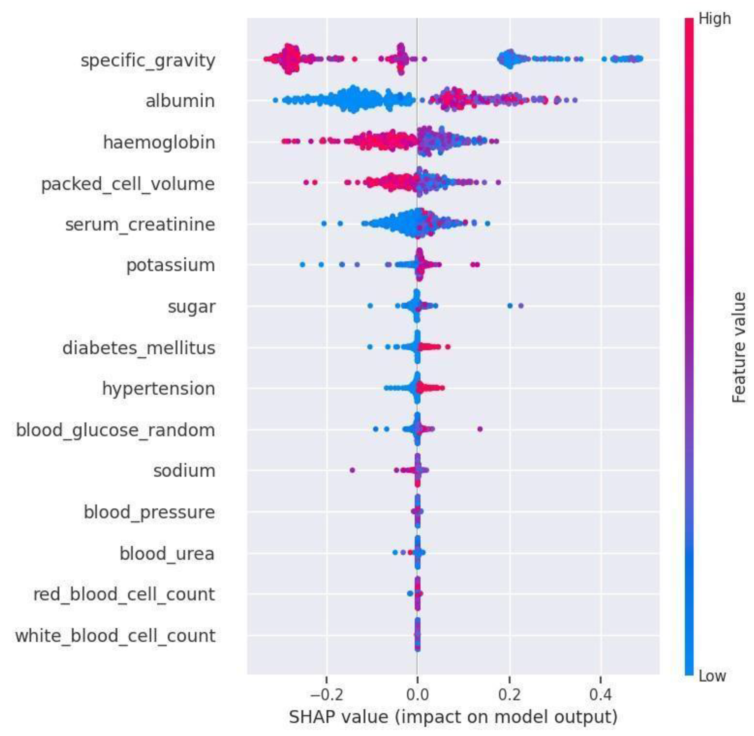
Feature significance methods generate a score for each input attribute of the model which indicates the attribute’s importance. A higher score denotes a higher contribution to the prediction. In
Figure 2, the x-axis of the Bee Swarm plot represents the attributes arranged in descending order of importance i.e., from high to low and the y-axis represents the SHAP values. The distribution of the attribute “specific_gravity” which spans between -0.375 and 0.475 is considered to be the widest distribution in the graph. Therefore specific_gravity is the most common cause for Diabetic Kidney Disease followed by albumin and hemoglobin. The distribution of the attribute “white_blood_cell_count” is lesser when compared to other attributes which make it the least impactful feature on Diabetic Kidney Disease. The feature importance value of the top 14 impactful attributes are tabulated in
Table 4.
4.2. Comparison of Performance of Machine Learning Models on Selected Features
The evaluation metrics values of the machine learning models which were trained and tested on the dataset with all features and selected features are represented in
Table 5 and
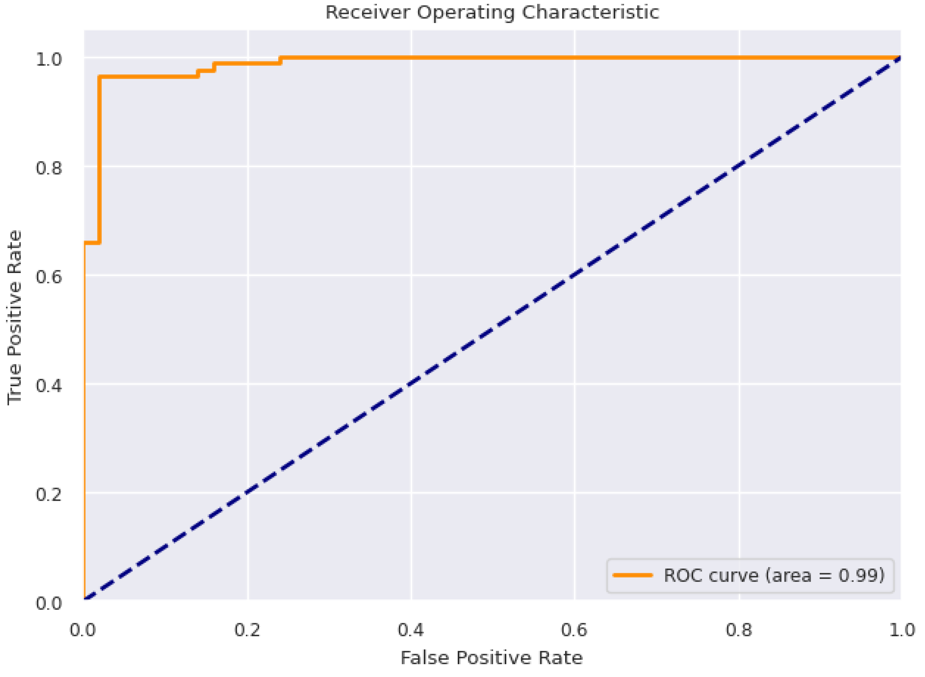
Table 6 respectively. Accuracy is used as the primary evaluation metric. The accuracy of LR, DT and RF remains constant before and after feature selection. Conversely, after applying feature selection, the BTM and SVM showed slight increase in accuracy. Using a subset of features during training, the Bagging Tree model produced the best accuracy of 96.29%. At 91.85%, Logistic Regression demonstrated the least accuracy. The Receiver Operating Characteristic Curve for BTM is represented in
Figure 3.
4.3. Comparison of Performance of Machine Learning Models after Optimization on Selected Features
Swarm Intelligence based optimization algorithms were used for hyperparameter tuning and the resultant hyperparameter values are tabulated in
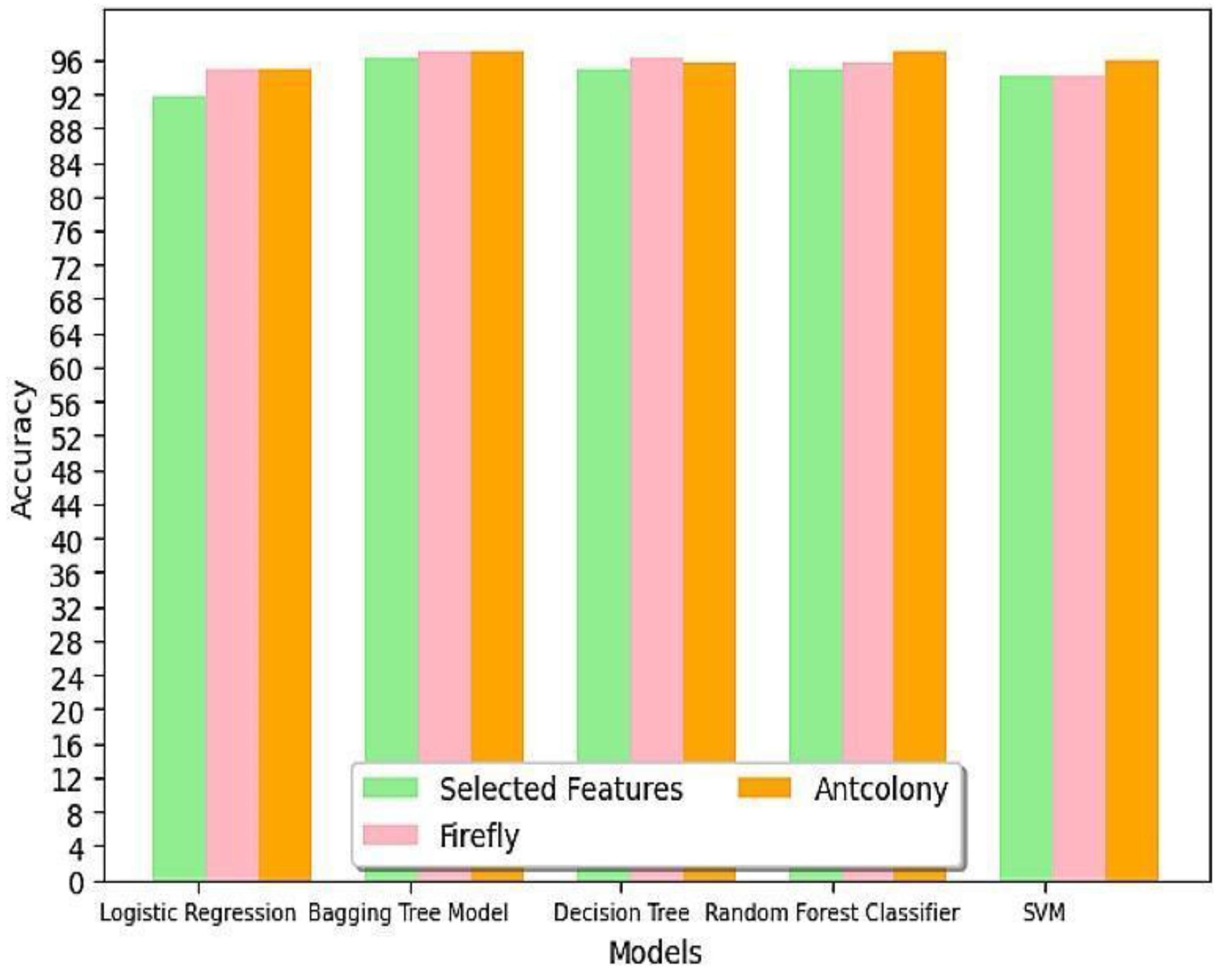
Table 7. The final model’s performance in predicting the likelihood of a patient developing Diabetic Kidney Disease is evaluated using various metrics. The analysis includes a comparison of accuracy among different classification models and the impact of optimization techniques on model accuracy. The accuracy values of different models under selected features with and without optimization are compared in
Table 8 and the same is represented as a graph in
Figure 4.
Logistic Regression: Both Firefly and Ant Colony Optimization increased the accuracy from 91.85% to 94.81%. Similar impact from both optimization algorithms.
Bagging Tree Model: Both Firefly and Ant Colony Optimization increased the accuracy from 96.29% to 97.03%. Similar impact from both optimization algorithms.
Random Trees: Firefly increased the accuracy from 94.81% to 96.29%, while Ant Colony increased it to 95.55%. Firefly performed better for Random Trees.
Random Forest: Firefly increased the accuracy from 94.81% to 95.55%, while Ant Colony increased it to 97.03%. Ant Colony performed better for Random Forest.
SVM: Firefly had no effect on the model, while Ant Colony increased accuracy from 94.07% to 96.00%.
Table 9 discusses the top 3 algorithms based on accuracy. Experimenting with selected characteristics, the highest accuracy of 97.03% was attained with the Bagging Tree Model with both PSO and ACO and Random Forest with ACO. From
Table 8, after optimization, SVM with FFO attained lowest accuracy of 94.07%.
5. Conclusion
The main objective of this research has been to empirically compare six different ML classifiers and find the best performing classification and robust classification model to effectively predict DKD early on. This study has explored the effect of feature selection techniques and swarm intelligence based optimization algorithms It was discovered that, when applied to the entire dataset, BTM and RF consistently produced the highest accuracy based on the empirical results produced by these algorithms. Notably, BTM performed the best overall throughout, although RF performed exceptionally well when optimization was used. Furthermore, augmenting the dataset with a larger and more diverse sample improves the model’s accuracy and real-time applicability, contributing to its overall robustness and viability for future research. Utilizing machine learning in the medical field will be rewarding both cost-wise, time-wise and most importantly reduces mortality and morbidity caused due to medical complications. Moreover, this implementation can be carried out with elementary hardware and software parameters. The finding of this study can be used to further develop models that forecast the progression of DKD in at-risk patients. Similar studies can be conducted on various disease related dataset to develop effective reliable disease prediction systems.
Data Availability Statement
References
- Available online: https://www.niddk.nih.gov/health-information/health-statistics/kidney-disease#:~:text=CKD%20is%20most%20common%20among,18%20to%2044%20(6%25).
- Available online: https://www.who.int/news-room/fact-sheets/detail/diabetes.
- Available online: https://www.ncbi.nlm.nih.gov/pmc/articles/PMC4170131/.
- S. Vijayarani, S. S. Vijayarani, S. Dhayanand et al., “Data mining classification algorithms for kidney disease prediction,” International Journal on Cybernetics & Informatics (IJCI), vol. 4, no. 4, pp. 13–25, 2015. [CrossRef]
- W. Gunarathne, K. W. Gunarathne, K. Perera, and K. Kahandawaarachchi, “Performance evaluation on machine learning classification techniques for disease classification and forecasting through data analytics for chronic kidney disease (ckd),” in 2017 IEEE 17th International Conference on Bioinformatics and Bioengineering (BIBE). IEEE, 2017, pp. 291–296.
- 2018. Available online: https://www.researchgate.net/publication/329395701_Prediction_of_Chronic_Kidney_Disease_Using_Machine_Learning_Algorithm.
- 2019. Available online: https://www.researchgate.net/profile/Revathy-Ramesh-3/publication/341398109_Chronic_Kidney_Disease_Prediction_using_machine_Learning_Models/links/5ebe42b1458515626ca85977/Chronic-Kidney-Disease-Prediction-using-Machine-Learning-Models.pdf.
- Rani KJ 2020 Diabetes prediction using machine learning. International Journal of Scientific Research in Computer Science Engineering and Information Technology. 6:294-305.
- Ifraz GM, Rashid MH, Tazin T, Bourouis S, Khan MM 2021 Comparative analysis for prediction of kidney disease using intelligent machine learning methods. Computational and Mathematical Methods in Medicine.
- Available online: https://www.ncbi.nlm.nih.gov/pmc/articles/PMC8772425/.
- Pal S 2023 Prediction for chronic kidney disease by categorical and non_categorical attributes using different machine learning algorithms.Multimedia Tools and Applications.82(26):41253-66.
- Kaur C, Kumar MS, Anjum A, Binda MB, Mallu MR, Al Ansari MS 2023 Chronic kidney disease prediction using machine learning. Journal of Advances in Information Technology.14(2):384-91.
- 1999. Available online: https://www.kaggle.com/datasets/abhia1999/chronic-kidney-disease/data.
- Ogunleye, A. and Wang, Q.G., 2019. XGBoost model for chronic kidney disease diagnosis. IEEE/ACM transactions on computational biology and bioinformatics, 17(6), pp.2131-2140.
- Wang, D. , Tan, D. and Liu, L., 2018. Particle swarm optimization algorithm: an overview. Soft computing, 22(2), pp.387-408. [CrossRef]
- Chu, C.C.F. and Chan, D.P.K., 2020. Feature selection using approximated high-order interaction components of the Shapley value for boosted tree classifier. IEEE Access, 8, pp.112742-112750. [CrossRef]
- Al Imran, A. , Amin, M.N. and Johora, F.T., 2018, December. Classification of chronic kidney disease using logistic regression, feedforward neural network and wide & deep learning. In 2018 International Conference on Innovation in Engineering and Technology (ICIET) (pp. 1-6). IEEE.
- Patel HH, Prajapati P 2018 Study and analysis of decision tree based classification algorithms. International Journal of Computer Sciences and Engineering.6(10):74-8.
- Biau G 2012 Analysis of a random forests model. The Journal of Machine Learning Research.13(1):1063-95.
- Kotsiantis SB, Tsekouras GE, Pintelas PE 2005 Bagging model trees for classification problems.Springer Berlin Heidelberg. InAdvances in Informatics.10th Panhellenic Conference on Informatics, PCI 2005, Volas, Greece, -13, 2005. Proceedings 10 2005. (pp. 328-337). 11 November.
- Wang L, editor 2005 Support vector machines: theory and applications. Springer Science & Business Media.
- Poli, R. , Kennedy, J. and Blackwell, T., 2007. Particle swarm optimization: An overview. Swarm intelligence, 1, pp.33-57.
- Dorigo M, Blum C 2005 Ant colony optimization theory: A survey. Theoretical computer science.344(2-3):243-78.
- Johari, N.F. , Zain, A.M., Noorfa, M.H. and Udin, A., 2013. Firefly algorithm for optimization problem. Applied Mechanics and Materials, 421, pp.512-517. [CrossRef]
|
Disclaimer/Publisher’s Note: The statements, opinions and data contained in all publications are solely those of the individual author(s) and contributor(s) and not of MDPI and/or the editor(s). MDPI and/or the editor(s) disclaim responsibility for any injury to people or property resulting from any ideas, methods, instructions or products referred to in the content. |
© 2024 by the authors. Licensee MDPI, Basel, Switzerland. This article is an open access article distributed under the terms and conditions of the Creative Commons Attribution (CC BY) license (http://creativecommons.org/licenses/by/4.0/).