Exploratory Spatial Analysis of Conservation Reserve Program Participation in the U.S. Midwest

1. Introduction

Since 1985, The Conservation Reserve Program (CRP) has been introduced as a supportive plan to incentivize environment-sensitive farm lands, where annual spendings on the plan have been expected to average $2.4 billion annually in fiscal years 2023–2032 Farm Bill [1]. The program’s success and cost-effectiveness heavily relies on voluntary participation from private landowners [2], as over 61% of U.S. land is privately owned [3]. Common motivations for participation include protecting natural resources, reducing soil erosion, improving water quality, providing wildlife habitat, and reflecting land stewardship or legacy values, especially among landowners with a strong conservation ethic [4,5,6]. The CRP compensates farmers for converting marginal lands to native vegetation and livestock producers for maintaining pasturelands. Enrollment restricts activities like farming and building, but landowners can resume these activities after the contract ends (typically after 10–15 years) [7]. Farmlands can be retired for two reasons, for conservation purposes and reducing the supply for their regular crops [6]. The midwestern regions have been the focus of many previous studies for CRP practices due to the row-crop production and high soil erosions in farmland compared to other US regions [6]. The US government adjusts the CRP participation caps according to changes in market conditions, and aiming not only for its environmental benefits, but also for managing crop supply [8]. This means that for example increased participation in CRP can lead to lower corn and soybean being available to the market and increasing their price whereas the decrease can have an opposite result [8,9].

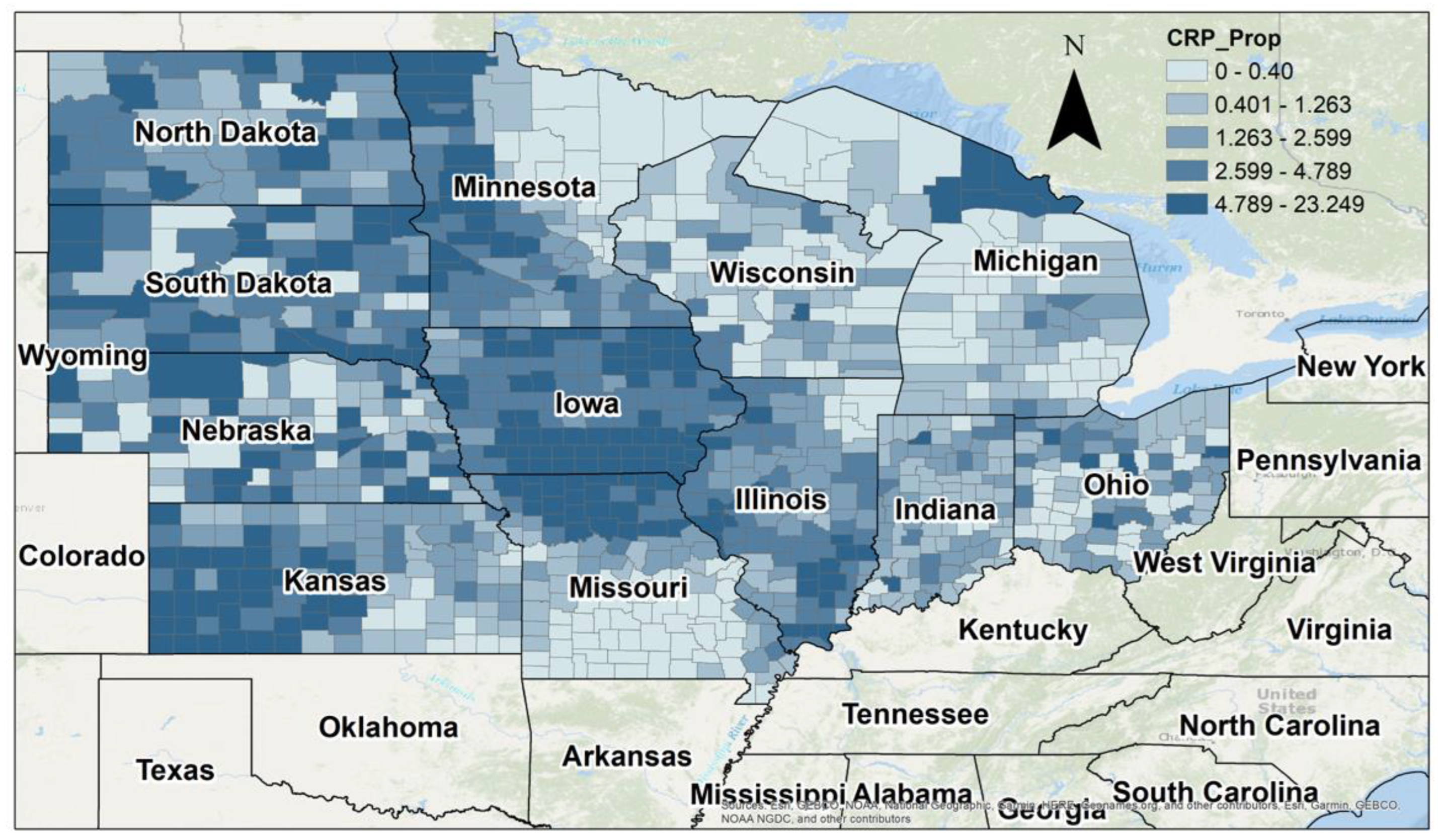
However, even among the Midwestern states and counties who may seem more homogenous compared to other US regions, there are significant differences in their participation in the CRP program, which makes it important to demystify such inconsistencies in such areas [10]. Figure 1 depicts some level of variances in CRP participation rates in the Midwest region.

In recent years, CRP participation has declined [11], which may have originated from several reasons, including lower competitiveness of the rental rates of the dedicated CRP farmlands compared to strong market conditions in the region [12], relatively high farm subsidy payments and risk management programs [7,8]. In summary, while CRP implementation policies and payments to farms play an important role in attracting more farmers into this environmentally friendly activity, factors such as land-use policies and local market conditions, including development pressure and rental demands, can work against CRP adoption [8]. While CRP has enrolled over 20 million acres nationwide, its effectiveness varies spatially due to unmodeled clustering in high row-crop counties, resulting in suboptimal targeting of erodible lands amid rising commodity prices [13]. While the impacts of policies and supplies on CRP participation have been extensively examined, there is a lack of studies to understand the spatial patterns that may exist in regional-like CRP adoption behaviors. More importantly, the recent decline in CRP enrollments and concerns about the spatial targeting and effectiveness of the program necessitate a systematic spatial evaluation of CRP adoption. This evaluation should determine whether CRP lands are spatially clustered and, if so, how these clusters relate to the characteristics of the lands. To address these gaps, this research seeks to answer the following questions:

• Is CRP participation spatially clustered across Midwestern U.S. counties, or is it randomly distributed? How about the spatial dependence of the contributing factors to CRP participation, such as CRP rental rates, soil erosion in cultivated farmlands, and farmland income per acre?
• Which counties exhibit statistically significant clusters of high and low CRP participation, and where are these clusters located? Are there any local deviations from the regional patterns regarding the CRP participation and each of the contributing factors?
• How do CRP rental rates, soil erosion, and agricultural profitability indicators spatially relate to CRP participation? Do these relationships demonstrate spatial clusterings?

Using county-level data on farmland characteristics, CRP participation, economic incentives, and soil erosion, this study applies an exploratory spatial data analysis (ESDA) to identify clustering patterns, spatial associations, and regional disparities in CRP enrollment across the Midwestern counties. To the best of our knowledge, this is fist study examining the CRP participation in the Midwest in such a detailed exploratory spatial analysis.

The results from this study would be helpful to the federal agencies and playmakers to understand the dynamics in the region in terms of the CRP adoption and any potential interference and association of other factors impacting the enrollments.

2. Materials and Methods

2.1. Case Study

This study is considering the US midwestern counties as the study area. The counties are from the Midwestern states, including consists of Illinois, Indiana, Iowa, Kansas, Michigan, Minnesota, Missouri, Nebraska, North Dakota, Ohio, South Dakota, and Wisconsin. Characterized as row-crop agriculture, substantial farmlands, and incurred by environmental pressure such as soil erosion on their cultivated farmlands, the region is well suited for examining the spatial patterns of CRP participation and associated land-use and economic characteristics. It is worth mentioning that counties are most detailed level of information publicly available regarding CRP participation in the US, as more accurate information such as the location of farms affiliated with CRP activities are prohibited to be shared by the federal government due to their confidentiality [14].

2.2. Data Sources and Variables

This section provides information regarding the data and variables used in the ESDA analysis. All the variables were harmonized based on the counties included in the study region.

The CRP participation rate and acreage for each county were extracted from the Farm Service Agency (FSA) web portal from which the average of CRP participation rate for years 2020 to 2024 were calculated [15]. To normalize the CRP participation rates in the study region, we divided them by farmlands acreage which were collected from the National Agricultural Statistics Service (NASS) for each of the corresponding state and counties [16]. The division resulted in the ratio of CRP participation acreage to total farmland acreage at the county level. This variable plays as the primary indicator of CRP adoption intensity, allowing reasonable comparisons between plans with different land bases.

This study also uses economic incentives and farm performance as other variables to capture both conservation-specific incentives and broader economic conditions influencing land-use decisions [6]. Average CRP rental rate plays as an important incentive factor in motivating farmers on deciding whether to contribute to the plan [6]. The corresponding data is collected from FSA web portal provided by USDA [15], and average of four year period consistent with CRP participation is considered for obtaining the variable’s values. Additionally, to examine the impact of general profitability of the farmlands in the study region, county-level income per acre was used as the primary economic productivity indicator instead of total net cash farm income. Unlike total income measures, income per acre standardizes economic returns by farmland area, enabling meaningful spatial comparison across counties of differing sizes and agricultural footprints. This measure better captures the opportunity cost faced by landowners when deciding between continued agricultural production and participation in CRP. This variable is collected from 2022 Census of Agriculture [16].

To reflect the environmental sensitivity of the farmlands, soil erosion in the study region, especially in the cultivated lands is collected [9]. The data is extracted from the NASS web portal, through the interactive Land Use & Cover Inventory Database (Lucid Public) [17,18]. The variable provides the average tons of the eroded soil per acre per year in the cultivated farmlands in each county.

2.3. Methodology

In this study, we employ ESDA to answer the research questions. This includes investigating spatial structure, clustering patterns, spatial associations of CRP involvements, as well as related agricultural, economic, and environmental variables across Midwestern counties. ESDA consists of a set of models purposed at describing and visualizing geographical distributions to detect any spatial outliers and atypical localizations [19,20,21]. The results helps to identify patterns of spatial association and indicate forms of spatial heterogeneity without imposing a predefined functional form or causal structure [19,20,22]. The ESDA framework is suitable for this study because CRP participation and agricultural outcomes are spatial, and ESDA framework can identify localized patterns, and provides links between spatial patterns and policy-relevant questions, supporting descriptive and diagnostic insights.

The ESDA workflow implemented in this study follows the following sequence:

• Determining a spatial weight matrix to specify spatial relationships
• Assessment of global spatial autocorrelation (Global Moran’s I)
• Identification of local clustering using Local Indicators of Spatial Association (LISA)
• Exploration of spatial co-location patterns using bivariate Local Indicators of Spatial Association (BiLISA).

The spatial analyses are conducted in Geoda 1.22.0.21 [21], in which statistical significance is assessed using 999 random permutations, with results reported at the 5% significance level to balance computational efficiency and statistical robustness.

2.3.1. Spatial Weights Matrix Specification

To incorporate the spatial dependence among observations in our dataset that come from counties in the study area, we modeled the relationships using spatial weights matrix. In this study, we use contiguity-based spatial weights matrix ($\mathrm{W}$), where counties are counted as neighbors if they share a boundary [23,24]. The spatial weights matrix is defined as:

$$w_{ij}=\left\{\begin{array}{c}1 \mathrm{if} \mathrm{counties} \mathrm{i} \mathrm{and} \mathrm{j} \mathrm{are} \mathrm{contiguous} \\ 0 \mathrm{otherwise} \end{array}\right.$$

(1)

where $\sum _j{w}_{ij}=1$. This row standardization ensures compatibility across counties with different number of neighbors [19,25]. The $\mathrm{W}$ obtained through this step will be used as the fundamental spatial interaction factor for all the subsequent spatial analyses in the framework.

2.3.2. Global Spatial Autocorrelation (Global Moran’s I)

Following the $w$ construction, Global Moran’s I evaluates the presence of overall spatial dependence and measures spatial autocorrelation. Global Moran’s I assesses whether values of a variable observed in nearby locations are more similar (or dissimilar) than would be expected under spatial randomness [19,23].

For a variable x, Moran’s I is defined as:

$$I={\displaystyle \frac{n{\sum }_i{\sum }_j{w}_{ij}\left(x_i-\overline{x}\right)\left(x_j-\overline{x}\right)}{S_0{\sum }_i{\left(x_i-\overline{x}\right)}^2}}$$

(2)

where n is the number of spatial units, $x_i$ represents the observed value of region i, $x_j$ represents the observed value of region j, and $\overline{x}$ is the mean of x. $w_{ij}$ is the spatial weight matrix, and

$${\mathrm{S}}_0={\sum }_{\mathrm{i}}{\sum }_{\mathrm{j}}{\mathrm{w}}_{\mathrm{i}\mathrm{j}}$$

(3)

When the value of I is greater than zero, it indicates a positive spatial correlation. This implies that regions with a high (low) level of for example CRP participation rate tend to cluster significantly in space, and vice versa. A positive and significant Moran’s I value indicates a general pattern of clustering in space of similar values, while negative values indicate spatial dispersion. Values close to zero suggest spatial randomness [19]. Monte Carlo permutation testing is used for inference in ESDA, randomly permuting observed values to generate a reference distribution under the null hypothesis of spatial randomness [19,21].

2.3.3. Local Indicators of Spatial Association (LISA)

To identify localized patterns, this study employs Local Indicators of Spatial Association (LISA). According to Anselin [19], the local Moran I statistic for county i can be defined as:

$${\mathrm{I}}_{\mathrm{i}}={\mathrm{z}}_{\mathrm{i}}\sum _{\mathrm{j}}{\mathrm{w}}_{\mathrm{i}\mathrm{j}}{\mathrm{z}}_{\mathrm{j}}$$

(4)

Where ${\mathrm{z}}_{\mathrm{i}}$represents standardized value at location i and ${\sum }_{\mathrm{j}}{\mathrm{w}}_{\mathrm{i}\mathrm{j}}{\mathrm{z}}_{\mathrm{j}}$is the spatial lag of neighboring values.

In this research, we run univariate LISA analyses for CRP proportion rates, CRP rental rates, soil erosion rates, and income per acre in cultivated farmlands. Through creating significance maps and clustering maps, LISA reveals statistically significant local clusters. These results directly address research questions addressing spatial heterogeneity of CRP participation, and the other contributing variables. LISA statistics identify four spatial regimes:

• High-High (HH) clusters: show counties with high values of given variable surrounded with other high value counties. This shows a spatial concentration in the clusters, suggesting strong regional consistency regarding the variable examined.
• Low-Low (LL) clusters: present counties with low values of the given variable surrounded with other low value counties. This depicts persistently low values in cluster/s for a given value, potentially indicating barriers/challenges for providing good conditions for the given variable.
• High-Low (HL) outliers: occur when counties with high values in a given variable are surrounded with low value counties. These are considered as spatial outliers, representing localized exceptions that deviate from the broader regional patterns.
• Low-High (LH) outliers: represent counties with low value in a given variable embedded in regions of high-value counties. This can signal under achievements of the variable-related potentials compared to neighboring counties’, triggering targeted policy interventions.

2.3.4. Bivariate Spatial Association

Following the identification of local spatial clustering patterns using univariate LISA analyses, bivariate local spatial association (BiLISA) analyses are employed to examine if county-level CRP participation is spatially associated with economic and environmental characteristics (represented by their corresponding variables) in neighboring counties. Unlike univariate LISA, which assess spatial dependence within a single variable, BiLISA evaluates the extent to which values of one variable at a given location are correlated with values of a different variable in surrounding locations (Anselin et al., 2006). Bivariate Moran’s I can be expressed as:

$${\mathrm{I}}_{\mathrm{i}}^{\mathrm{x}\mathrm{y}}={\mathrm{z}}_{\mathrm{x},\mathrm{i}}\sum _{\mathrm{j}}{\mathrm{w}}_{\mathrm{i}\mathrm{j}}{\mathrm{z}}_{\mathrm{y},\mathrm{j}}$$

(5)

where $z_{x,i}$ represents the standardized value of variable x at county i, $z_{y,j}$ represents the standardized value of variable y in neighboring counties (j), and $w_{ij}$ represents elements of the spatial weight matrix.

3. Results and Discussion

This section presents the findings of the analyses conducted for each of the methodologies discussed in the methodology section. Additionally, it provides discussions of the results, elucidating the managerial insights and implications derived from the analyses.

3.1. Global Spatial Autocorrelation

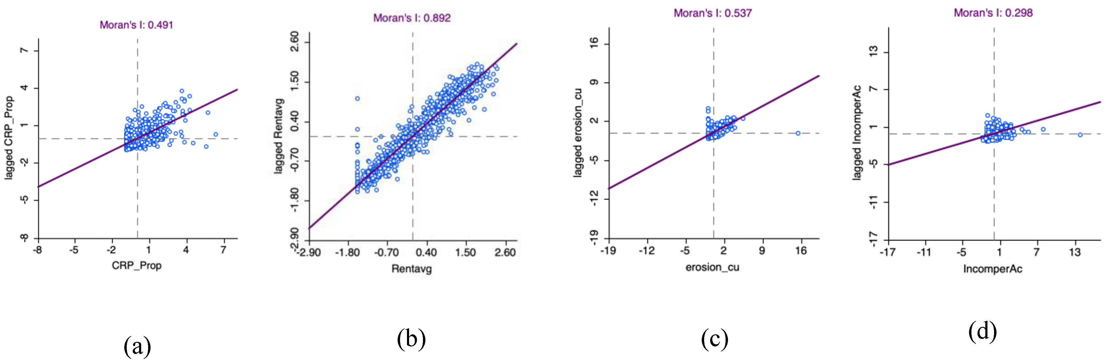
In this section, we provide the results from employing Global Moran’s I to examine if the four variables’ values cluster spatially or are randomly distributed. Figure 2 presents the Global Moran’s I scatter plots for four county-level variables across the Midwestern United States: (a) CRP proportion, (b) average CRP rental rates, (c) soil erosion on cultivated land, and (d) farm income per acre. All analyses were conducted using a first-order queen contiguity spatial weights matrix. The spatial weight was created based on a variable referring to the counties’ FIPS codes.

Based on Figure 2(a), the Global Moran’s I statistic for county-level CRP proportion is 0.491, indicating a moderate and positive spatial autocorrelation, suggesting counties with relatively high (low) CRP participation tend to be surrounded by counties with similarly high (low) CRP participation. This value for the CRP rental rates variable (Figure 2(b)) results 0.892, indicating very strong positive spatial autocorrelation, meaning CRP rental payments are highly spatially structured, with counties offering high rental rates neighboring other high CRP rent counties, and vice versa.

Resulted 0.537 from the Global Moran’s I statistic for soil erosion on cultivated land, Figure 2(c) indicates moderate-to-strong positive spatial autocorrelation. This implies counties with higher erosion rates tend to cluster spatially, which may originate from shared biophysical conditions such as soil characteristics and climate. However, Figure 2(d) reports a weaker Global Moran’s I value for farm income per acre variable, indicating a lower spatial autocorrelation compared to other variables, but still positive and offering some degree of clustering.

Taken together, all variables exhibited statistically significant positive spatial autocorrelation, indicating that location-based dynamics influence adoption outcomes. Stronger spatial clustering in CRP rental rates and soil erosion risk supported their inclusion in subsequent spatial interaction analyses (LISA and BiLISA), though potential misalignments between these variables and CRP participation remain. However, the lower Moran’s I value for income per acre suggests weaker regional clustering and greater regional heterogeneity.

3.2. Local Spatial Autocorrelation Analysis (LISA)

At this stage, LISA is employed to identify county level spatial heterogeneity for each of the variables. The LISA significance map determines, for a examined variable, where the spatial clustering or outlier behavior is unlikely to happen randomly (statistically significant). Additionally, the LISA cluster map shows and interprets the local spatial patterns of persistent high and low values of a variable, with also detecting outliers, showing localized deviations from regional trends.

3.2.1. Local Spatial Autocorrelation of CRP Participation

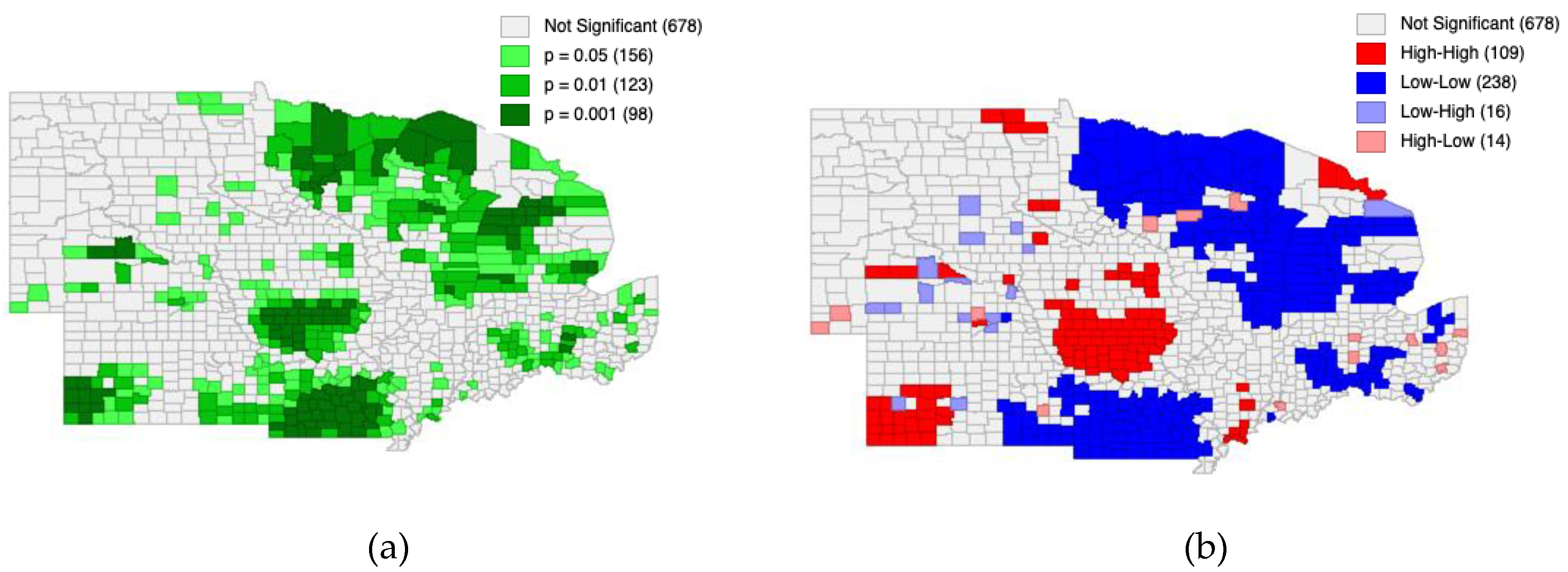
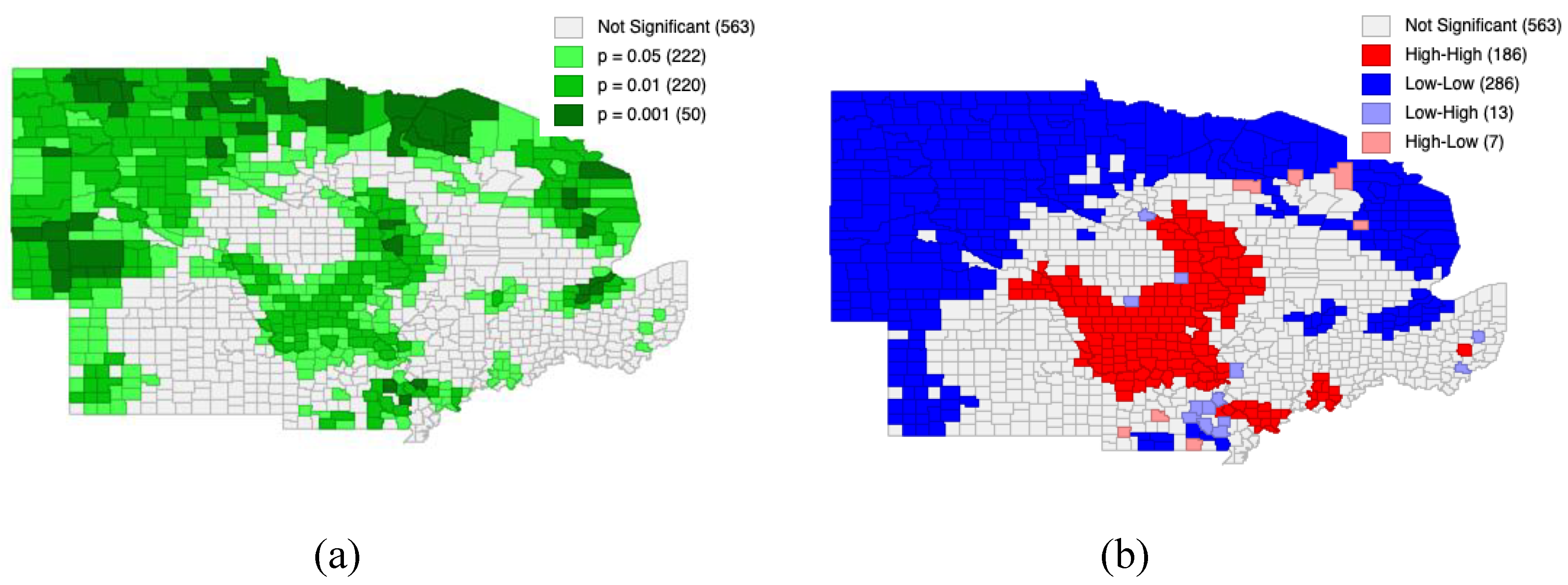
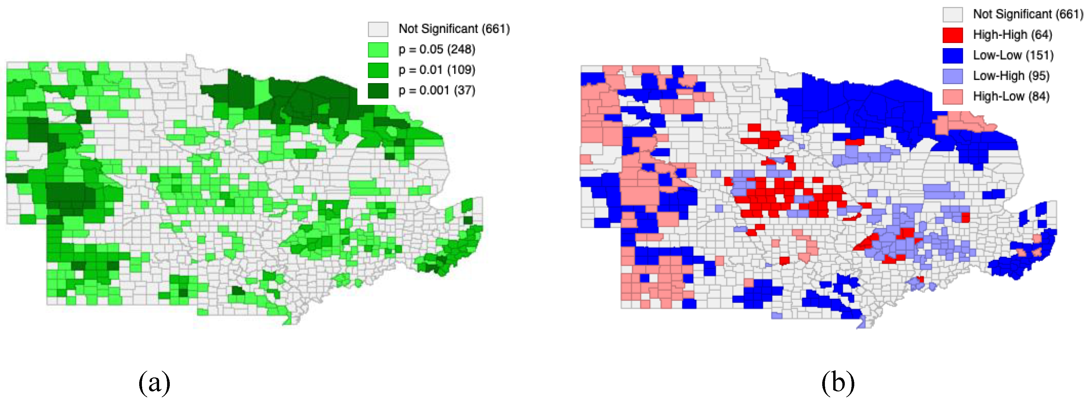
LISA was calculated for CRP proportion variable using the local Moran’s I statistic based on a first-order queen contiguity spatial weights matrix, using 999 random permutations, with results reported at the 5% significance level. The resulted two maps from the analysis are provided in Figure 3.

The LISA significance map in Figure 3(a) reveals that CRP participation has statistically significant local spatial autocorrelation across multiple subregions, while many counties show no statistically significant local association, reflecting spatial heterogeneity in program participation. In Figure 3(b), the LISA cluster map identifies distinct spatial regimes of CRP participation, with HH clusters representing counties with high CRP rates surrounded by similarly high-participation neighbors, representing contiguous high CRP enrollments. LL clusters, presented in the map, indicate areas where low CRP participation persists across neighboring counties, suggesting spatially entrenched non-participation or alternative land-use priorities.

The existence of these two types of clusters implies that that CRP participation is more driven by regional dynamics rather than isolated county-level decisions. However, HL and LH clusters turn out to be spatially scattered, indicating a small number of localized deviations from regional participation trends occurring. This echoes the CRP participation alignment in the study region with broader regional patterns rather than local anomalies.

3.2.2. LISA for CRP Rental Rate

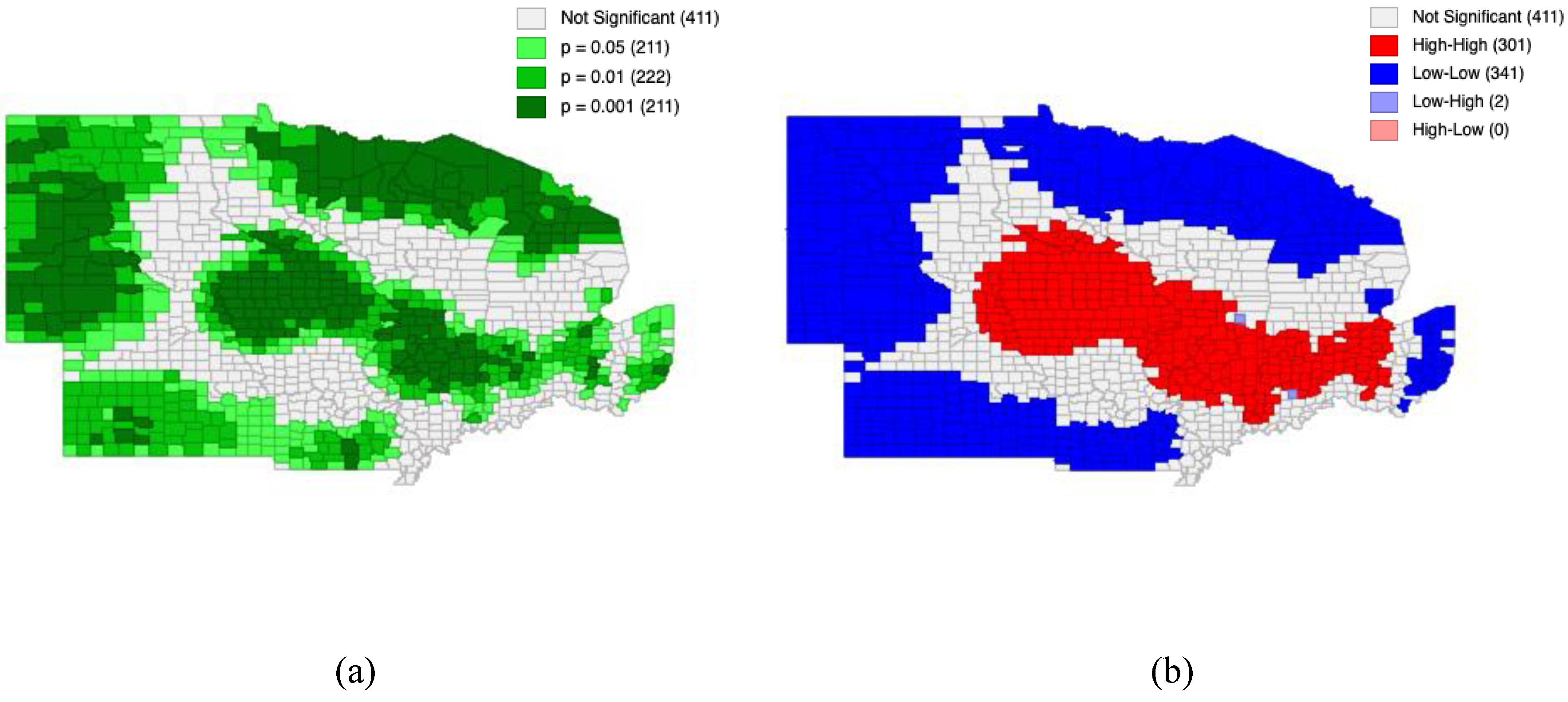
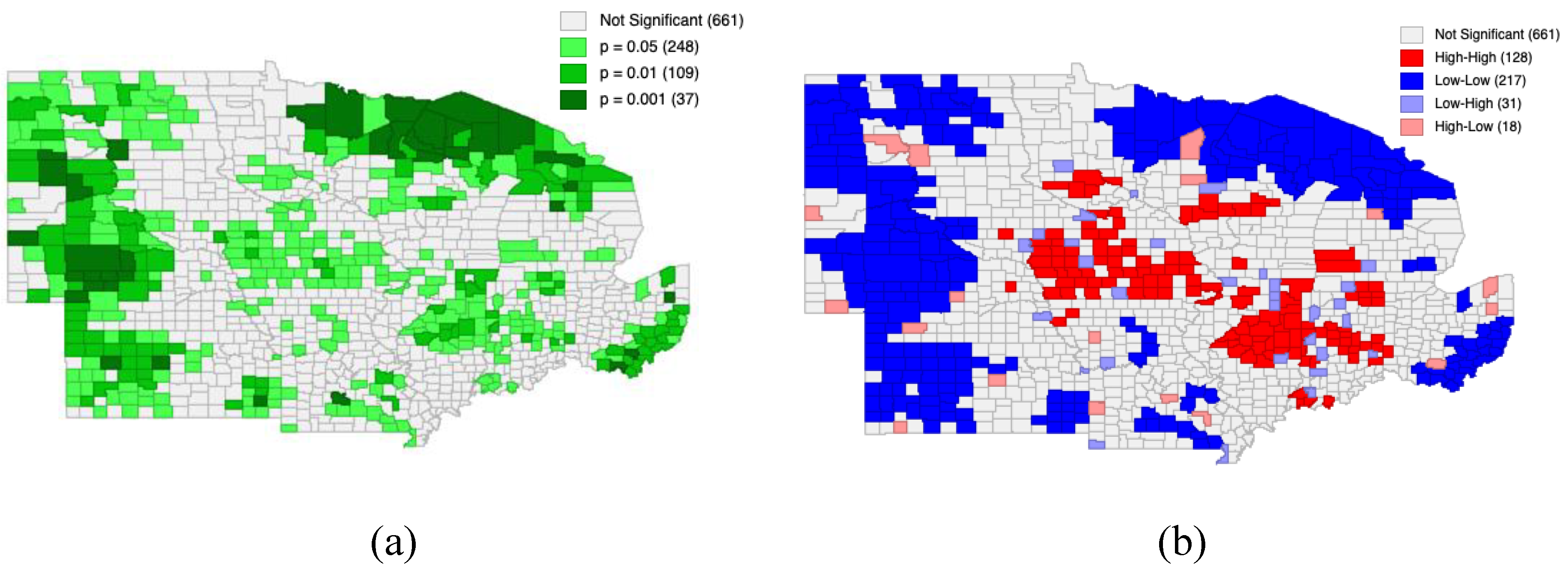
Already indicated strong positive spatial autocorrelation across the Midwest, CRP rental rates were also examined by LISA to identify the specific locations of the clusters and spatial regimes where such clustering occurred. LISA significance and cluster maps are presented in Figure 4 to show statistically significant local patterns in CRP rental payments.

Figure 4(a) depicts that statistically significant clustering occurs across large, contiguous areas. Also, a higher proportion of counties is significant compared to the result from CRP participation which implies stronger spatial structuring of rental payments than CRP enrollment patterns in the Midwest. Regarding the cluster map, the clusters of both HH and LL form broad contiguous significant clusters, indicating that rental rate determination reflects strong regional patterns. Comparing to CRP participation, more counties display significant local clustering, implying CRP rental payments are more spatially structured and regionally consistent. However, regarding the outliers in the map, they are comparatively rare, meaning very low localized deviation from the dominant HH and LL rental payment regions.

3.2.3. LISA for Soil Erosion on Cultivated Farmlands

This subsection examines the local spatial autocorrelation of soil erosion on cultivated farmlands to assess whether erosion risks exhibit spatial clustering across Midwestern counties.

The LISA significance map in Figure 5(a) demonstrates that numerous counties exhibit statistically significant local spatial autocorrelation in soil erosion, indicating that soil erosion distributions are spatially structured rather than randomly distributed. The LISA cluster map in Figure 5(b) reveals significant regional clustering through HH and LL clusters with comparatively rare spatial outliers. The prevalence of HH and LL clusters in the region suggests that soil erosion is driven by regional scale factors rather than anomalies in isolated counties.

3.2.4. LISA of Income per Acre on Farmlands

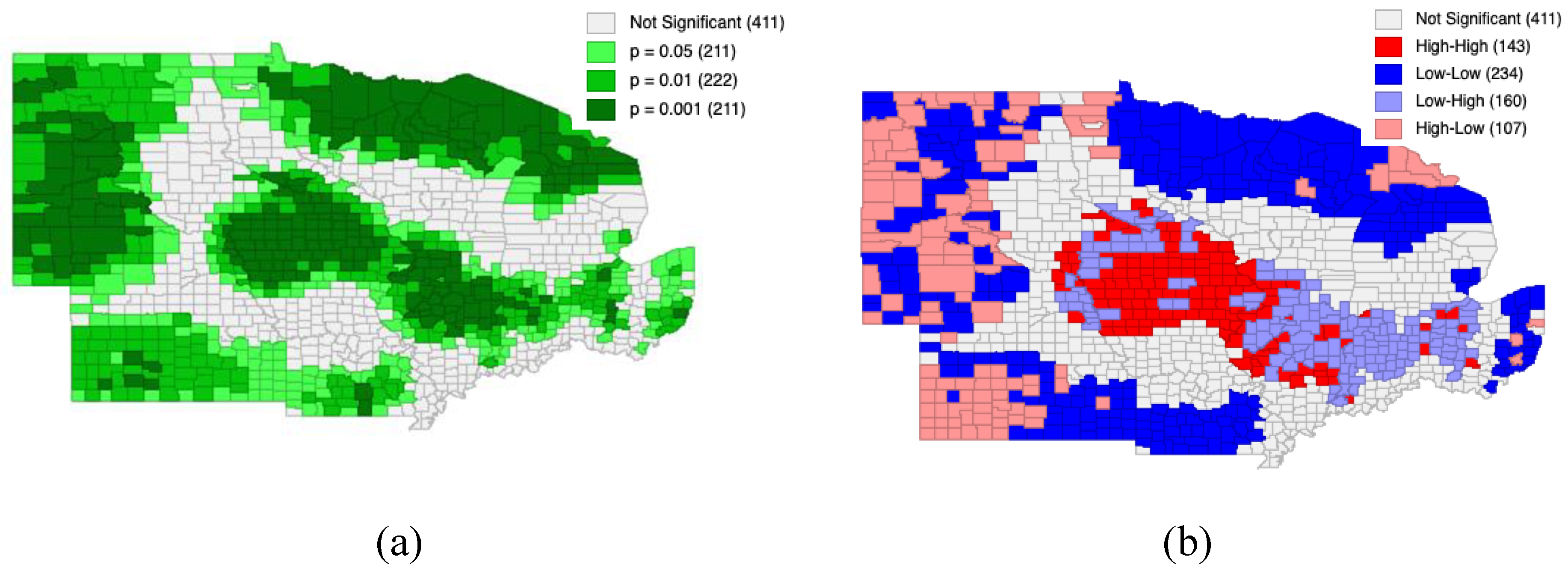
This subsection analyzes the local spatial structure of farm income per acre using LISA. The results of the analysis, including the significance map and cluster map, are provided in Figure 6.

The LISA significance map in Figure 6(a) indicates that 394 out of 1,055 counties show statistically significant local spatial autocorrelation in income per acre. The cluster map in Figure 6(b) indicates evident patterns of spatial clusters. LL clusters represent contiguous areas. There are also limited number of outliers (HL and LH), suggesting that localized variations from regional income patterns are relatively uncommon. The spatial clusters for income per acre of cultivated farmlands can be caused by dominant regional production systems and product mixes, variations in land quality and agronomic potential, and differences in market access and supporting infrastructure.

3.3. BiLISA Between CRP Participation and Economic & Environmental Factors

In the following subsections, following the detection of local spatial patterns for each of the variables using LISA, we proceed with employing BiLISA to examine whether spatial patterns of CRP participation are spatially associated with neighboring economic and environmental conditions, thereby proving insights regarding spatial co-location patterns between CRP participation and key drivers.

3.3.1. BiLISA between CRP Participation and CRP Rental Rates

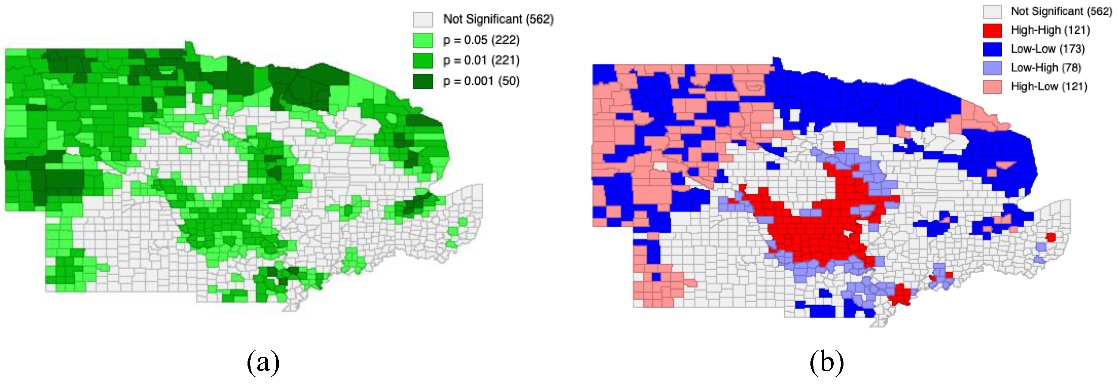
This subsection provides results from BiLISA regarding the identifying of local spatial patterns between CRP participation and CRP rental rates. The significance map and cluster maps are provided in Figure 7.

According to the results demonstrated in Figure 7(a), it can be observed that large, spatially contiguous areas of significant counties are formed, indicating statistically significant CRP participation-CRP rental rates relationship operates systematically across the study region, and CRP participation patterns being spatially linked to rental rates in neighboring counties.

The results in Figure 7(b) shows several extensive and statistically significant spatial clustering across the region. More specifically, HH clusters appear in the central Midwest, indicating counties with high CRP participation surrounded by neighbors offering relatively high rental rates, indicating an effective alignment between participation and rental rates in these counties. LL clusters are present parts of the northern, southern, and eastern Midwest, reflecting limited incentive-driven CRP adoption. There also exist outlier (HL and LH) clusters in the western and eastern Midwest, respectively, presenting high and low participation rates coincided with low and high rental payments, respectively, suggesting that factors beyond rental payments, such as opportunity costs, land suitability, or institutional constraints, may encourage or inhibit enrollments.

3.3.2. BiLISA between CRP Participation and Soil Erosion

In this section, BiLISA maps are used to identify localized spatial patterns between CRP proportion and soil erosion on cultivated lands across Midwestern counties. The results from significance map and cluster map are provided in Figure 8.

According to the results in Figure 8(a), a considerable number of counties indicate statistically significant local spatial associations between CRP participation and soil erosion in cultivated farmlands. More specifically, Figure 8(b) shows HH clusters, primarily concentrated in the central Midwest, whereas LL clusters are also present with relatively low erosion, but still low participation, both cluster types showing partial alignment between CRP enrollment and erosion-related environmental pressure. However, spatial outliers also exist in the region, presenting spatial heterogeneity in local areas (also presented in Figure 8(b) with LH and HL labels in the legend). Specially, the coexistence of HH regions with LH regions around it highlights the importance of considering the incorporation of more differentiated economic and institutional variables into their CRP policy design, as the high erosion rate in such counties is not resulting in high enrollments.

3.3.3. BiLISA between CRP Participation and Income per Acre

In this subsection, BiLISA is employed to examine the local spatial association between county-level CRP participation and income per acre on neighboring farmlands.

The BiLISA significance map in Figure 9(a) indicates that clusters of counties show spatial dependence between CRP enrollment and surrounding farmland income conditions. The corresponding cluster map in Figure 9(b) reveals alignment between high/low participation and high/low local profitability (income per acre), whereas the existence of LH and HL clusters highlight spatial mismatches. Together, these patterns suggest that while CRP participation aligns with income conditions in some regions, the relationship varies spatially across the Midwest.

The non-uniform occurrence of CRP participation across the profitability of the farms in the Midwest is pronounced in the HH, LL, and spatial outlier clusters, offering some implications. As for the HH clusters, the results imply that CRP through rental payments may function as a complementary income-stabilization mechanism rather than a substitute for low profitability. On the other hand, LL clusters with relatively low participation and income may have been impacted by potential barriers to enrollment or reduced program’s attractiveness. Regarding the spatial mismatches (HL and LW clusters), their presence implies that uniform CRP rental rates or enrollment criteria may not fully account for different counties’ economic conditions.

4. Conclusion

4.1. Summary of Key Findings

This study carried out ESDA to examine county-level patterns of CRP participation across the Midwestern United States. Using Global Moran’s I analyses, the results uncovered that none of the CRP participation, rental incentives, soil erosion, and farm income per acre are randomly distributed across the Midwest, though with varying intensity regarding their spatial significance and farm income per acre displaying weaker but still meaningful spatial structure.

Local spatial analyses (BiLISA) further disclosed distinct HH and LL clusters for each variable, illustrating pronounced regional heterogeneity in CRP adoption, and its contributing variables, demonstrating that CRP participation is spatially associated with both neighboring rental incentives and environmental and economic conditions of the counties. However, spatial mismatches were more intense where high erosion risk or strong financial indicators did not coincide with high CRP enrollment.

Additionally, to discover significance of spatial relationships between CRP participation and other variables, BiLISA analyses were conducted, unraveling uneven relationships across space. While in parts of the Midwest the plan was working in tandem with local conditions, such as HH clusters in the central Midwest where high-CRP counties were surrounded with neighboring counties benefiting high rental rates, spatial mismatches also appeared, implying other factors rather than the controlled variable vs. participation could have affected such events.

4.2. Policy Implications

The findings from this study have several important implications for the design and targeting of conservation policy. First, from the difference between the highly significant spatial clustering of CRP rental rates relative to more moderate clustering in CRP participation, it can be inferred that while rental rates are highly regionally patterned, CRP participation rates do not always respond proportionally, implying that uniform incentive mechanisms may not be equally effective throughout various regions and counties in the Midwest. Second, despite the partial alignment of CRP participation with soil erosion risk, as demonstrated by HH clusters, there are spatial outliers where CRP participation occurs despite relatively lower erosion risk, and vice versa. This can motivate the opportunities for designing more spatially targeted conservation policies that better prioritize such environmentally sensitive areas. Overall, these results stress the need to adopt a spatially differentiated policy design approach in CRP planning. It is expected that accounting for spatial spillovers and regional clustering could improve both the environmental effectiveness and the economic equity of the plan.

4.3. Limitations and Future Research

This study is subject to several limitations. First, due to the confidentiality restrictions on farm-level CRP enrollment, the spatial analyses in this study were all run based on county-level data for each of the variables, which may have masked important variations that may have existed in sub-county or farm-level. Therefore, applying the framework to other areas with a finer scale of data being available, such as parcel or farm level, could uncover micro scale cluster, helping better understand spatial patterns. Second, ESDA is inherently descriptive, thereby mainly being used for detecting or verifying spatial patterns in a given region; therefore, it does not examine the presence of causal relationships. Not considered a limitation, but it is important to recognize the technique’s role and value in detecting anomalies and patterns, which would consequently initiate causal analyses (spatial econometric models). Additionally, considering a broader set of variables in another spatial analysis could potentially enrich understanding of the local CRP enrollments. Moreover, applying the framework to other US regions could help examine the generalizability of this study’s findings.

References

- Coppess, J.; Swanson, K.; Paulson, N.; Schnitkey, G.; Zulauf, C. Reviewing the Latest CBO Farm Bill Baseline. farmdoc daily 2022, 12. [Google Scholar]
- Thapa, B.; Chapagain, B.P.; McMurry, S.T.; Smith, L.M.; Joshi, O. Understanding Landowner Participation in the Conservation Reserve Program in the U.S. High Plains Region. Land Use Policy 2024, 141, 107163. [Google Scholar] [CrossRef]
- USGS Protected Areas Database of the United States (PAD-US): Version 1.4 2016.
- Dayer, A.A.; Lutter, S.H.; Sesser, K.A.; Hickey, C.M.; Gardali, T. Private Landowner Conservation Behavior Following Participation in Voluntary Incentive Programs: Recommendations to Facilitate Behavioral Persistence. Conservation Letters 2018, 11, e12394. [Google Scholar] [CrossRef]
- Ranjan, P.; Church, S.P.; Floress, K.; Prokopy, L.S. Synthesizing Conservation Motivations and Barriers: What Have We Learned from Qualitative Studies of Farmers’ Behaviors in the United States? Society & Natural Resources 2019, 32, 1171–1199. [Google Scholar] [CrossRef]
- Egerson, D.; Thornton, B.S.; Thompson, D.; Westlake, S.M.; McConnell, M.D.; Evans, K.O. A Rapid Mapping Review of Studies on the Motivations and Barriers to Participation in the Conservation Reserve Program. Society & Natural Resources 2025, 38, 1146–1168. [Google Scholar] [CrossRef]
- Conservation Reserve Program (CRP) | Farm Service Agency. Available online: https://www.fsa.usda.gov/resources/programs/conservation-reserve-program (accessed on 14 December 2025).
- Yu, J.; Goodrich, B.; Graven, A. Competing Farm Programs: Does the Introduction of a Risk Management Program Reduce the Enrollment in the Conservation Reserve Program? Journal of the Agricultural and Applied Economics Association 2022, 1, 320–333. [Google Scholar] [CrossRef]
- Hendricks, N.P.; Er, E. Changes in Cropland Area in the United States and the Role of CRP. Food Policy 2018, 75, 15–23. [Google Scholar] [CrossRef]
- Allen, A.; Vandever, M. Conservation Reserve Program (CRP) Contributions to Wildlife Habitat, Management Issues, Challenges and Policy Choices—An Annotated Bibliography. Scientific Investigations Report, 2012. [Google Scholar]
- GAO Conservation Reserve Program: Improving How USDA Selects Land Could Increase Environmental Benefits | U.S. GAO; 2024.
- Taylor, M.R.; Hendricks, N.P.; Sampson, G.S.; Garr, D. The Opportunity Cost of the Conservation Reserve Program: A Kansas Land Example. Applied Economic Perspectives and Policy 2021, 43, 849–865. [Google Scholar] [CrossRef]
- Cattaneo, A. Balancing the Multiple Objectives of Conservation Programs; 2006. [Google Scholar]
- USDA - National Agricultural Statistics Service - About NASS - Agency Overview. Available online: https://www.nass.usda.gov/About_NASS/ (accessed on 20 December 2025).
- Conservation Reserve Program (CRP) Statistics | Farm Service Agency. Available online: https://www.fsa.usda.gov/tools/informational/reports/conservation-statistics/crp (accessed on 20 December 2025).
- 2017 Census by State | 2022 Census of Agriculture | USDA/NASS. Available online: https://www.nass.usda.gov/Publications/AgCensus/2022/Full_Report/Census_by_State/index.php (accessed on 20 December 2025).
- LUCID. Available online: https://www.nrisurvey.org/lucid/ (accessed on 20 December 2025).
- Frontuto, V.; Corsi, A.; Novelli, S.; Gullino, P.; Larcher, F. The Visual Impact of Agricultural Sheds on Rural Landscapes: The Willingness to Pay for Mitigation Solutions and Treatment Effects. Land Use Policy 2020, 91, 104337. [Google Scholar] [CrossRef]
- Anselin, L. Local Indicators of Spatial Association—LISA. Geographical Analysis 1995, 27, 93–115. [Google Scholar] [CrossRef]
- Haining, R. Spatial Data Analysis in the Social and Environmental Sciences; Cambridge University Press: Cambridge, 1990; ISBN 978-0-521-44866-6. [Google Scholar]
- Anselin, L.; Syabri, I.; Kho, Y. GeoDa: An Introduction to Spatial Data Analysis. In Handbook of Applied Spatial Analysis: Software Tools, Methods and Applications; Fischer, M.M., Getis, A., Eds.; Springer: Berlin, Heidelberg, 2010; pp. 73–89. ISBN 978-3-642-03647-7. [Google Scholar]
- Ye, X.; Wu, L. Analyzing the Dynamics of Homicide Patterns in Chicago: ESDA and Spatial Panel Approaches. Applied Geography 2011, 31, 800–807. [Google Scholar] [CrossRef]
- Cliff, A.D.; Ord., J.K. Spatial Processes : Models & Applications; Pion, 1981. [Google Scholar]
- Spatial Econometrics: Methods and Models | Springer Nature Link (Formerly SpringerLink). Available online: https://link.springer.com/book/10.1007/978-94-015-7799-1 (accessed on 20 December 2025).
- LeSage, J.; Pace, R.K. Introduction to Spatial Econometrics; Chapman and Hall/CRC: New York, 2009; ISBN 978-0-429-13808-9. [Google Scholar]