Submitted:
25 December 2025
Posted:
26 December 2025
You are already at the latest version
Abstract
Rolling horizon energy management systems (EMS) and model predictive control (MPC) for microgrids in smart cities face a fundamental trade-off: finer temporal discretization improves operational characteristics but rapidly increases the size of the optimization problem and execution time, jeopardizing real-time feasibility. Furthermore, in short-horizon operation, only the first control actions are implemented, while long-horizon decisions primarily guide feasibility and constraints. This paper proposes a computation-aware temporal mesh design layer that jointly selects a variable granularity of blocks and an optimisation horizon, explicitly bounded by market-aligned settlement steps and per-cycle computation budgets. Candidate configurations are represented as pairs ⟨B, H⟩, where B is a constant-pass block programme, and H is the horizon, and are uniquely tracked through an auditable mesh signature. The method first evaluates a predefined, market-consistent set to establish reproducible cost and execution time benchmarks, then applies a Greedy-Value-of-Information (Greedy-VoI) search that generates valid neighbouring meshes through local refinement, thickening, and resolution reallocation without breaking the horizon mosaic or admissible step sizes. All candidates are evaluated using the same microgrid use case and the same comparative KPIs, enabling the systematic identification of near-optimal mesh-horizon designs for practical EMS implementation.
Keywords:
energy management system (EMS)
; model predictive control (MPC)
; rolling horizon
; variable temporal granularity
; greedy algorithm
; value of information (VoI)
; non-uniform time mesh
; microgrid scheduling
; compute-aware optimization
1. Introduction
Electric power systems are being reshaped into the smart grid paradigm, characterized by bidirectional power and information flows, the rapid expansion of variable renewable generation and distributed energy resources (DER) along the grid, together with the widespread deployment of advanced metering, sensing, communications, and automation technologies [1]. This transition offers a significant route to decarbonization, not only by displacing fossil fuel-based electric generation but also by electrifying end-uses—most notably space and water heating—where high-efficiency heat pumps can deliver low-carbon heat [2]. At the same time, the proliferation of behind-the-meter PV, storage, EV charge points, and electric flexible loads or consumption assets increases operational complexity in distribution grids, with documented concerns such as reverse power flows, voltage deviations/unbalance, and protection challenges under high PV penetration [3], as well as local grid congestions [4]. Consequently, system “flexibility”—the ability to shift or modulate generation, consumption, and storage in response to external signals—has become a central enabling resource for integrating high shares of variable renewables while preserving security of supply and compliance with network constraints [5,6]. In particular, demand-side management can convert electrified loads into controllable resources that follow price, carbon-intensity, or grid operator signals, ranging from tariff-driven load shaping to direct, real-time control of smart loads and DER portfolios [7]. Energy Management Systems provide the supervisory layer that operationalises such flexibility by acquiring field data, forecasting and optimally scheduling heterogeneous DER and controllable loads to meet multiple objectives—e.g., minimizing operating costs, maximizing self-consumption, or minimizing emissions—while respecting user preferences and grid/market constraints; this role is well established in microgrid supervisory control and is increasingly relevant in the emerging prosumer-centric market paradigm [8,9].
To take advantage of the flexibility and controllability of distributed energy resources presupposes a high degree of automation in monitoring, optimisation and actuation, because evidence from residential demand-response programmes shows that engagement is hindered by perceived complexity and effort, as well as concerns about risk and loss of control; accordingly, automation becomes an enabling condition when accompanied by transparency and user final control [10]. In line with these insights, the stakeholder-centric surveys conducted in the REEFLEX project report that only 39.8% of respondents currently use any energy management/monitoring tool and only 19% use a dedicated energy/flexibility management tool, while simultaneously revealing strong preferences—sometimes unanimous—for fully automated solutions with user override capabilities and for trust-building features such as long-term support and automatic security updates (with higher expectations of automatic control for critical loads) [11]. An EMS can therefore be defined as a supervisory hardware–software layer that acquires measurements and contextual data, forecasts relevant disturbances (e.g., weather, occupancy and prices) and solves an optimisation problem subject to technical and contractual constraints to schedule and dispatch controllable generation, flexible demand and storage, thereby meeting local objectives (cost, comfort or emissions) while enabling the provision of grid or market services [7,8]. Such EMS concepts span residential home EMS, commercial and tertiary Building EMS, industrial EMS, and microgrid/community controllers. Across these domains, Model Predictive Control (MPC) is widely adopted as a core algorithmic paradigm because its receding-horizon formulation explicitly embeds forecasts and operational constraints and has been extensively validated for both building HVAC energy management and microgrid operation optimisation [12,13].
In EMS/MPC based on deterministic optimisation techniques, the dominant sources of performance degradation are driven mainly by imperfect forecasts of exogenous inputs (e.g., weather, demand, renewable generation, and prices) and by discretisation of continuous dynamics and device operating modes into granular decisions on a fixed time grid [13,14,15,16]. The receding or rolling horizon principle partly mitigates forecast uncertainty by repeatedly updating the optimisation as new measurements and forecasts become available, thereby correcting operation schedules before prediction errors accumulate [14,15]; likewise, increasing the temporal granularity of the EMS (e.g., 15-min intervals instead of hourly steps) can reduce discretisation artefacts and better capture intra-hour variability, ramping behaviour, and constraint activation—although at the cost of a larger optimisation problem with higher computation needs [12,17]. However, finer granularity increases the number of decision variables and constraints roughly proportionally to the number of time steps. It can cause solve times to rise sharply with problem size, particularly in mixed-integer EMS formulations, where the combinatorial growth in binary variables is a significant factor [18]. In complex, large-scale deployments (e.g., microgrids or aggregated DER portfolios), this computational burden can make real-time operation impractical, leading to the paradox that the computation time exceeds the control interval so that the “optimal” solution becomes outdated before it can be applied [18].
To address the increasing computational needs that arise from complex EMS/MPC formulations, particularly when discretized at finer time steps, the literature has proposed several strategies. A proposed solution is to decompose long-horizon (some days) mixed-integer scheduling problems into a sequence of overlapping subproblems (a few hours) solved in a rolling-horizon manner, which can deliver substantial runtime reductions for large energy-hub Mixed Integer Linear Programming(MILP) formulations while preserving the quality of the resulting operating policies [19]. Beyond fixed periodic re-optimization, the rolling-horizon execution itself can also be made adaptive: [20] proposes a dynamic scheduling tool that selects informative start times for the rolling-horizon solves under uncertainty—rather than triggering them uniformly—thereby improving operational performance in a microgrid energy management case study. In parallel, temporal aggregation of input time series—via clustering into typical time steps or typical periods (e.g., typical days/weeks)—reduces the number of time steps and can be tuned to the mathematical structure of the optimization model (notably the presence of time-linking constraints such as storage); recent comparative studies formalize the accuracy–runtime trade-off as a Pareto frontier and provide methods to identify near-optimal aggregation configurations instead of relying on ad hoc choices [21,22]. Another alternative is multi-rate discretization, in which different decision variables and constraints are represented at distinct (and potentially time-varying) temporal resolutions according to their characteristic dynamics; the fully flexible temporal resolution formulation proposed by [23] explicitly enables per-variable resolutions and demonstrates computational-efficiency gains in large-scale co-optimization of investment and operational decisions (see Figure 1). Finally, the computational budget is also shaped by EMS design choices, such as the length of the optimization horizon. Multi-objective receding-horizon scheduling studies suggest that longer optimization horizons can enhance renewable utilization and operational outcomes, albeit at a higher computational cost, thereby reinforcing the motivation for adaptive update policies and multi-resolution modeling in practical EMS deployments [24]. More generally, variable-granularity schemes—where temporal resolution is adjusted during execution—are emerging as another approach to address the computational needs related to complex EMS/MPC formulations.
Variable temporal granularity (also referred to as flexible temporal resolution or multi-timescale discretization) can be defined as the deliberate use of non-uniform time steps along the optimization horizon—and, in some formulations, different time steps for different decision variables—so that fast dynamics and near-term decisions are represented with acceptable resolution. In contrast, slower trends and far-future decisions are represented more coarsely to reduce problem size. In EMS/MPC settings, this concept is especially natural because the controller is usually executed in a receding or rolling horizon structure, where forecasts and states are updated frequently and only the first portion of the computed optimal trajectory or operation set-points are implemented before re-optimizing; consequently, modelling fidelity is most valuable near the current time, whereas distant decisions mainly provide feasibility and boundary guidance. A basic justification for variable granularity is also offered by the exponential decay of sensitivity (EDS). Under suitable regularity conditions, the sensitivity of the optimal decision at stage i to perturbations at stage j can be bounded to decay exponentially with the temporal distance ∣i-j∣ [25]. In rolling-horizon EMS/MPC—where near-term actions are executed, and the horizon is repeatedly shifted—EDS implies that aggregating or coarsening far-future time steps may have limited impact on the current control action, while still capturing long-term constraints and dominant trends. This rationale is directly exploited in diffusing-horizon MPC, which constructs a discretization grid whose spacing becomes exponentially sparser as the horizon is extended, achieving substantial computational savings with limited closed-loop performance degradation [26].
Multi-timescale rolling operation schemes for building and integrated energy systems exemplify this idea by combining day-ahead schedules with progressively finer intraday and real-time refinements (e.g., hourly → 15-min → 5-min) [27], and by embedding horizons with increasing step size directly into MPC to balance economic performance, robustness, and runtime [28]. Closely related multi-horizon formulations also seek long look-ahead horizons without an explosion in variables, e.g., distributed MPC for networks of energy hubs [29] and multi-resolution approaches for storage control that explicitly trade temporal/state resolution against computation, allowing re-optimization to be performed more frequently [30]. Beyond EMS, flexible temporal resolution has recently become an explicit computational lever in large-scale MILP scheduling, such as network-constrained unit commitment with adaptive time-period aggregation [31] and cost-oriented time-adaptive UC formulations [32], reinforcing the broader observation—quantified in comparative studies of temporal-resolution selection—that higher temporal fidelity improves representation accuracy but can quickly render optimization impractical at scale [33].
Although temporal aggregation and resolution-selection have been studied in planning-oriented energy system models, the methodological development for operational microgrid EMS/MPC—where computational latency becomes a hard real-time constraint—remains comparatively limited [20]. Recent contributions nevertheless illustrate the potential of non-uniform temporal designs: [35] introduces an “optimal rolling-horizon strategy” (ORoHS) that explicitly partitions prediction/execution horizons to trade off dispatch cost and forecast accuracy under uncertainty. At the same time, diffusing-horizon MPC provides a constructive coarsening mechanism in which sampling points become progressively sparser (e.g., exponentially) as they move farther into the horizon, leveraging the fact that far-future perturbations have a weaker influence on near-term control actions [20]. In parallel, time-adaptive discretization is also emerging in large-scale mixed-integer scheduling problems (e.g., unit commitment), where cost-oriented temporal resolution seeks to retain fine granularity only where it is economically consequential [20]. However, most existing works either (i) evaluate a limited set of preselected discretizations, or (ii) prescribe coarsening rules tailored to a specific formulation, and they rarely provide general methods to compute an optimal variable-granularity design for a given microgrid and operating context; moreover, to the best of our knowledge, the coupled design problem of jointly selecting both a variable time-mesh and the rolling-horizon length in an integrated and systematic manner is still largely unaddressed in the EMS literature. Building on the above gaps, this work aims to take a step further by proposing a compute-budget-aware procedure that evaluates admissible optimization-horizon lengths, along with block-structured variable granularities tailored to the target market setting. Then, it employs a Greedy-Value-of-Information (Greedy-VoI) metaheuristic to generate and screen new mesh–horizon combinations. In doing so, the proposed methodology targets microgrid-specific near-optimal temporal designs that explicitly balance closed-loop economic performance, forecast uncertainty, and real-time solvability.
The remainder of this paper is organized as follows. Section 2 presents the proposed methodology, including the problem formulation, the design choices adopted for variable temporal granularity and optimization horizon selection, and the evaluation procedure. Section 3 reports the main results obtained across the considered case study. Section 4 discusses the findings, highlighting the observed practical implications and limitations. Finally, Section 5 summarizes the main conclusions and outlines directions for future research.
2. Materials and Methods
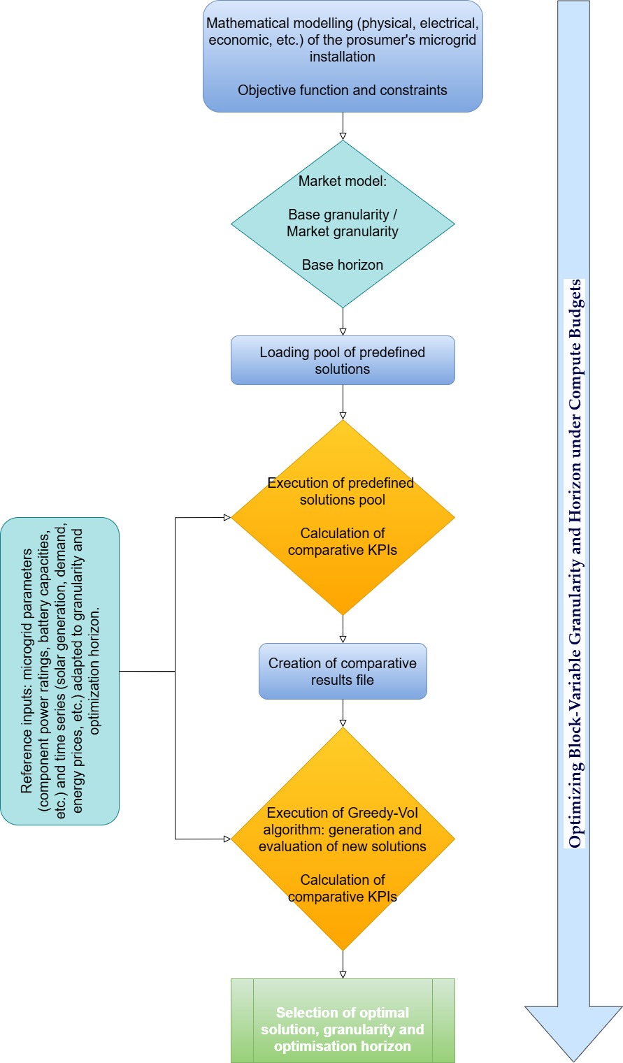
This section introduces the proposed methodology for optimal selection of a block-variable temporal discretization and an optimization horizon for rolling horizon EMS/MPC operation under explicit computational constraints. First, the microgrid modelling layer (objective function and constraints) and the market layer are outlined, which define the admissible settlement-aligned time steps and candidate horizon lengths. Next, the workflow is described in Figure 2, where a pool of market-consistent “baseline” discretizations is evaluated to build a comparable KPI benchmark, which is then used to guide a metaheuristic search. Finally, the high-level logic of the Greedy-VoI procedure is presented, which is used to generate and assess new discretization–horizon candidates, as well as the criteria used to select the final recommended configuration.
At a high level, the proposed procedure can be interpreted as a compute-aware time-mesh design layer placed on top of a conventional EMS optimizer. The starting point is a mathematical model of the prosumer microgrid, which includes electrical/physical constraints, as well as economic terms, along with a set of reference inputs (e.g., demand, PV generation, electricity prices, and device limits) representative of the operating period of interest. The market layer then provides the practical boundaries of the decision space: (i) a base/market granularity consistent with market clearing and settlement, and (ii) a base horizon that reflects how far ahead the EMS is expected to plan. These elements define the admissible combinations of “how often decisions are made” (temporal resolution) and “how far ahead the EMS looks” (horizon). At the same time, a compute budget constrains what is feasible to solve repeatedly in real time.
The workflow in Figure 2 proceeds in two stages. In the first stage, the method loads and executes a pool of predefined solutions, i.e., a curated set of block schedules and horizons that are directly compatible with the target market structure. Each candidate is run through the same evaluation pipeline: a rolling-horizon simulation (or repeated replanning procedure) is executed, only the first control action is applied at each step, and the process is repeated across the study horizon. For each candidate configuration, the framework computes comparative KPIs that capture both operational quality and computational practicality. The output of this stage is a consolidated results dataset that provides a transparent baseline and a cost–runtime reference for subsequent search.
In the second stage, the Greedy-VoI algorithm iteratively generates and evaluates new candidate discretizations beyond the predefined pool. Conceptually, Greedy-VoI explores local modifications of the time mesh—such as refining near-term blocks (where actions are executed) and coarsening far-term blocks (where decisions primarily provide boundary guidance)—and may also test alternative horizon lengths to ensure market alignment and computational limits at all times. After each candidate is generated, it is evaluated through the same execution and KPIs, and the best-performing configurations are retained according to the selected decision rule. The procedure finishes when the compute budget and/or stopping criteria are met, returning the selected optimal solution together with its recommended block schedule (granularity profile) and optimization horizon, ready to be deployed as the EMS planning configuration for the specific microgrid and market framework.
2.1. Mathematical definition of granularity, blocks, and optimisation horizon
This section provides a mathematical definition of the blocks that form the EMS/MPC optimisation horizon, as well as the parameters that characterise them and the equations they must satisfy. The pair defines each solution that makes up an optimisation horizon:
⟨B,H⟩,
Where , is a schedule of time blocks and is the optimization horizon. A time-block schedule is an ordered list of blocks:
B={(n1,Δt1),…,(nB,ΔtB)}
Where block comprises consecutive time steps (granularities) of identical duration (minutes).
For auditability, the mesh signature is defined as:
sig(B,H)=[(n1,Δt1)…(nB,ΔtB);H]
2.1.1. Optimization horizon
The optimization horizon (minutes) is
and the effective size of the discrete problem is
2.1.2. Conditions that must be met by the combinations of values that define the optimization horizons.
Unless extended for a specific application (e.g., allowing 30′ in 15′ markets), there is a limited group or set of admissible time-step (granularities):
- {5, 15, 60} [minutes] for 15-minute settlement markets
- {15, 60, 120} [minutes] for 1-hour settlement markets
- Integer blocks and closure of the horizon:
This constraint ensures that the blocks tile the horizon exactly.
- Horizon domain:
H∈H, H={2880,4320} (2 or 3 days in minutes)
Project pre-defined horizon lengths are 2 or 3 days (h), other works could propose other optimization horizons
- Model-size bound:
Nmax is chosen from solver and hardware limits (e.g., 220–300 periods for MILP with mixed integer devices). It is the first control against intractable instances.
- Real-time calculations:
It is enforced a per-cycle compute budget (seconds) with
- Non-decreasing resolution:
Δt1≤Δt2≤…≤ΔtB
This avoids repeated switching fine→coarse→fine, which tends to generate unstable set points and redundant solver work.
2.1.3. Predefined pool of solutions
As previously indicated, some solutions adapted to the electric market environment have been defined and tested before applying the Greedy-VoI algorithm to ensure that these market solutions are evaluated. Table 1 presents this predefined market of solutions.
2.1. Greedy-VoI Algorithm
Greedy-VoI frames time-mesh and horizon selection as a constrained discrete design problem over candidate signatures , where is a schedule of blocks (each block containing consecutive steps of duration ) and is the optimization horizon. The induced discrete size is and , subject to market-admissible step sizes, exact tiling of the horizon, monotone coarsening along the horizon , and real-time feasibility constraints (e.g., and per-cycle solver time ). Over this feasible set, each candidate s, is evaluated through a rolling-horizon execution to obtain an operational KPI (e.g., total cost or penalty-augmented cost) and a computational metric . Greedy-VoI then applies a greedy, value-of-information principle by prioritizing modifications that provide the largest marginal improvement per unit computational “expense”, e.g.,
Where is obtained from via an elementary mesh operator (refine, coarsen, or reallocate resolution across blocks, optionally combined with a horizon change) and avoids division by zero. A greedy choice based on marginal gains is theoretically motivated in settings that exhibit diminishing returns, where selecting the best incremental move at each iteration yields provable near-optimality for submodular objectives—a property that, while not guaranteed in EMS/MPC mesh design, provides a principled rationale for using marginal-gain criteria to guide a metaheuristic search.
Operationally, the algorithm starts from a small pool of market-consistent baseline meshes and selects an incumbent that is feasible under . At iteration , a neighborhood is generated by applying admissible mesh transformations (e.g., refining the near-term blocks where set-points are executed, and compensating by coarsening far-term blocks to preserve feasibility), producing a set of candidates . Each is either (i) screened using lightweight proxies (e.g., expected change in or predicted ) and/or (ii) fully evaluated by running the rolling-horizon EMS to obtain and . The next iterate is chosen greedily as among candidates that respect the compute constraints; the incumbent is updated when improves (or when a selected dominance rule improves a cost–time trade-off frontier). A key structural justification for focusing refinement near the beginning of the horizon is that, in rolling-horizon control, only the first decisions are implemented, and then the problem is re-solved; moreover, sensitivity to far-future discretization typically decreases with temporal distance. This intuition is consistent with the diffusing-horizon time-coarsening rationale—where the grid becomes progressively sparser farther into the horizon (often exponentially)—which has been shown to reduce computational effort while preserving near-term control quality in MPC.
2.1. Tool testing
It is essential to emphasize that the procedure or algorithm developed is agnostic with regard to the microgrid in which the EMS is to be implemented, meaning that this methodology can be applied to all types of real-world installations. “Appendix A—Optimization model” describes the optimization algorithm and microgrid used in this article; however, any other model, optimization method, or installation to be managed could be used.
The tool has been developed, implemented, and tested in the PYTHON environment, using these main libraries:
- PYTHON, version 3.9
- PANDAS, version 2.3.3
- NUMPY, version 2.0.2
- ORTOOLS, version 9.14.6206 (solver)
The running platform’s main characteristics are:
- 11th Gen Intel(R) Core (TM) i7-1165G7 @ 2.80GHz (2.80 GHz)
- 16 GB RAM
3. Results
This section presents the experimental results and validation of the proposed compute-aware time-mesh design procedure on the selected microgrid case study. The results are reported by comparing (i) the predefined pool of market baseline configurations and (ii) the additional candidates generated by the Greedy-VoI search. Performance is quantified through comparative KPIs that jointly capture operational quality and computational practicality: optimization results and execution time.
The algorithm described has been applied to the optimisation scenario described in “Appendix A – Optimisation model” in which, as indicated, the objective function is to minimise the operating costs of an isolated electric and hydrogen vehicle charging station. The objective function aims to reduce costs, so a negative value of the objective function implies a positive revenue.
As can be seen in the It can also be observed that solution [(4x15), (23x60), (24x120); 4320], in addition to giving the best objective function result, has the shortest execution time of the three-day solutions.
It can therefore be observed that the ideal solution from the pool of predefined solutions, [(4x15), (23x60), (24.120); 4320], improves the results of a basic solution for an hourly market, [(72x60); 4320]: the optimum is 0.37% better, but the execution time is 42.11% of the resolution time of the reference solution.
Table 2 in Figure 3 and Figure 4, the best solution among the ones proposed in the predefined solution pool, is also the best solution of the optimisation horizon of 3 days and is the one identified as [(4.15), (23x60), (24.120); 4320], while for the case with a 2-day optimisation horizon, it is identified as [(4x15), (23x60), (12x120); 2880].
It can also be observed that solution [(4x15), (23x60), (24x120); 4320], in addition to giving the best objective function result, has the shortest execution time of the three-day solutions.
It can therefore be observed that the ideal solution from the pool of predefined solutions, [(4x15), (23x60), (24.120); 4320], improves the results of a basic solution for an hourly market, [(72x60); 4320]: the optimum is 0.37% better, but the execution time is 42.11% of the resolution time of the reference solution.
Figure 4 confirms the fact that a greater number of steps implies a longer execution time. No direct relationship is observed between the computational cost and the number of steps involved.
This phenomenon is also evident in Figure 5, which displays the results of applying the Greedy-VoI algorithm to this use case and hourly market. It can be seen that optimisation horizons with a greater number of steps imply a longer execution time, although no direct relationship is observed. It should be noted that to generate the 300 solutions evaluated and shown in Figure 5, the conditions shown in equation (10) must be met, and the maximum number of blocks must be greater than 3.
As indicated in Section 2, after evaluating the solutions proposed in the predefined solution pool, the Greedy-VoI algorithm is applied to search for a better solution providing 300 solutions. Among the better solutions obtained, the next can be obtained because they are the best for one, two and three blocks starting with 5-minutes, 15-minutes and 1-hour steps:
-
3 days optimization horizon, one block in 2-hour steps (H4320|B1|[36x120])
- ○
- Optimization result: -110.891 €
- ○
- Execution time: 0.067 sec (36 steps)
-
3 days optimization horizon, two blocks in 1-hour and 2-hour steps (H4320|B2|[2x60;35x120])
- ○
- Optimization result: -110.891 €
- ○
- Execution time: 0.04 sec (37 steps)
-
3 days optimization horizon, three blocks in 15-minutes, 1-hour and 2 hours steps (H4320|B3|[4x15;1x60;35x120])
- ○
- Optimization result: -110.891 €
- ○
- Execution time: 0.039 sec (40 steps)
-
3 days optimization horizon, three blocks in 5-minutes, 15-minutes and 2-hour steps (H4320|B3|[3x5;7x15;35x120])
- ○
- Optimization result: -110.891 €
- ○
- Execution time: 0.055 sec (45 steps)
These solutions have a very similar objective value, and one must go beyond the fourth decimal place to find differences, which may be due to the discretization process and granularity adaptation errors in the input signals. These solutions slightly improve the objective function by 0.09% compared to the best solution in the predefined solution pool (-110.793€) and maintain similar overall execution time values.
It is important to note that the best solutions proposed by the Greedy-VoI algorithm, in addition to improving the objective value, maintain a much shorter execution time compared to slower solutions of the 300 provided by the algorithm:
-
3 days optimization horizon, three blocks in 5-minute, 1-hour and 2-hour steps (H4320|B3|[24x5;8x60;31x120])
- ○
- Optimization result: -110.890 €
- ○
- Execution time: 0.153 sec (63 steps)
-
3 days optimization horizon, two blocks in 5-minute and 2-hour steps (H4320|B2|[48x5;34x120]])
- ○
- Optimization result: -110.890 €
- ○
- Execution time: 0.16 sec (82 steps)
-
3 days optimization horizon, two blocks in 1-hour and 2-hour steps (H4320|B2|[48x5;34x120]
- ○
- Optimization result: -110.891 €
- ○
- Execution time: 0.228 sec (46 steps)
As can be seen, despite having similar ‘optimisation results’ to those of faster execution solutions, execution times are up to 5 times longer.
It is important to highlight the stability of the proposed solutions and, consequently, the consistency of the proposed method. Interesting details can be observed after a detailed analysis of the 300 solutions:
-
Optimization result [€]:
- ○
- Minimum: -110.89142
- ○
- Average: -110.85491
- ○
- Maximum: -110.38627
- ○
- Standard deviation: 0.07465
-
Execution time [sec]:
- ○
- Minimum: 0.032
- ○
- Average: 0.105
- ○
- Maximum: 0.228
- ○
- Standard deviation: 0.0541
Across all evaluated configurations for the analysed use case, the optimisation outcomes are stable while execution times are more variable:
- The objective results reach a minimum of −110.8914€, a maximum of -110.38627€ with a mean of −110.8549€ and a standard deviation of 0.0747€, which corresponds to a coefficient of variation of ~0.067% (0.0747/110.8549). This indicates a very close clustering around the best solution, most candidates deliver near-identical economic performance.
- Executions times range from 0.032 s to 0.284 s, with a mean of 0.105 s and a standard deviation of 0.054 s, i.e., a coefficient of variation of ~51% (0.054/0.105). This larger relative spread is consistent with computational effort being more sensitive to discretisation size and mesh structure than the objective value itself.
The proposed workflow is useful for selecting solutions that achieve good optimisation results with lower and more predictable execution times, confirming that the method is stable and consistent.
When analysing the pool of predefined solutions for 15-minute markets (Table 3), a similar trends can be observed to those of the predefined solutions for hourly markets. The solution that combines 5-minute, 15-minute and hourly blocks in a 3-day horizon, [(3x5),(95x15),(48x60); 4320], provides a better solution (-110.424€) with the shortest execution time (0.666 sec) for this optimisation horizon (3 days / 4320 minutes) than an homogeneous solution based on market inputs, [(288x15); 4320]. Shorter optimization horizon solutions provide faster results, but worse optimization results.
The use of the Greedy-VoI algorithm provides an improved result:
-
3 days optimization horizon, 3 blocks in 5-minutes, 1- hour and 2-hour steps (H4320|B3|[12x5;31x60;20x120]
- ○
- Optimization result: -110.793€
- ○
- Execution time: 0.275 sec (63 steps)
4. Discussion
This section discusses the results from an engineering and deployment-oriented perspective, focusing on how the time-mesh design (in terms of the number of steps and block structure) and the optimisation horizon affect economic performance and computational effort under market-alignment constraints.
A key practical insight is that temporal granularity directly controls two error sources. First, the discretisation error decreases as Δt is reduced, and second, a finer mesh reduces the forecast-induced error in the optimisation layer. However, this improved fidelity comes at the cost of a larger optimization problem (more steps → more variables/constraints), where execution time increases with the number of steps. Even if the present case study does not show critical runtimes, this scaling behaviour becomes decisive for larger formulations (more assets, more binaries, additional network constraints) or for embedded/edge EMS platforms with limited computing capabilities.
Within this context, Figure 5 illustrates the value of a variable-resolution design: Greedy-VoI explores market-valid neighbours that reallocate resolution across the horizon (e.g., refining near-term blocks where actions are executed and coarsening the tail where decisions mainly provide boundary guidance). This produces configurations that can improve (or match) the objective while explicitly controlling the number of steps and, consequently, solver time. From a deployment perspective, the primary outcome is not a single “best Δt”, but rather a systematic approach to identifying a mesh–horizon pair that achieves near-optimal economics while remaining compatible with the available compute budget and the market settlement structure.
The dispersion of the optimisation results across the market feasible mesh–horizon candidates is very small relative to the objective magnitude, which supports the stability and consistency of the proposed selection workflow. In particular, the objective exhibits a tight clustering (CV ≈ 0.067%), suggesting that multiple market-feasible meshes deliver equivalent economic performance. In contrast, execution time shows a higher spread (CV ≈ 51%), which aligns with the expected sensitivity of solver effort to discretization size (steps) and block structure rather than to the operating cost itself.
5. Conclusions
This work is motivated by a persistent gap in the deployment of EMS/MPC. While high temporal fidelity / low granularity can reduce forecast and discretization-induced errors and improve results, complex microgrid formulations become computationally prohibitive when solved repeatedly in rolling-horizon operation. In rolling horizon control, only the first set-points are implemented before re-optimization, which means that the time discretization should be treated as a design variable rather than a fixed modelling choice: it must be sufficiently fine where actions are executed, and constraints are likely to bind, and increasingly coarse where decisions primarily serve as feasibility and boundary guidance.
Accordingly, this paper presents a general, market-aware methodology for co-designing the EMS time mesh and the optimization horizon under explicit real-time constraints. The approach formalizes each candidate configuration as a pair ⟨B, H⟩, introduces an auditable mesh signature to represent block schedules uniquely, and enforces practical feasibility conditions such as admissible time steps, exact horizon tiling, and a per-cycle compute budget. Building on this formulation, the proposed workflow first benchmarks a pool of predefined market-consistent solutions. Then, it applies the Greedy-VoI procedure to generate and evaluate new candidates using the same KPIs, enabling the systematic identification of near-optimal discretization–horizon combinations for a given microgrid and market framework.
In the presented case study, the search yields multiple market-feasible configurations whose economic performance is very close, while exhibiting apparent differences in discretization size (i.e., the number of steps) and observed solving time. This supports two practical conclusions. First, the methodology is effective as a design aid: it can systematically propose and rank deployable ⟨B, H⟩ options that balance objective quality with computational effort, avoiding ad hoc choices of Δt and horizon. Second, even when the optimisation is not yet runtime-limited, treating the time mesh as a controllable design variable remains valuable because it provides a transparent way to anticipate scalability limits and to select conservative configurations for future expansions (additional assets, tighter binaries, network constraints) or for execution on constrained hardware. Overall, the proposed workflow operationalizes the intuition that the “best” EMS discretization is not necessarily the finest one, but the one that achieves near-optimal economics within market and compute constraints, with resolution concentrated where it yields the highest value of information.
A key outcome of the experimental validation is the high stability of the recommended mesh–horizon designs: across a large set of market-feasible candidates, the optimization results remain tightly concentrated around the best solution, while runtime varies substantially with steps and block structure. This indicates that, for the studied use case, the proposed workflow reliably finds multiple “economically equivalent” configurations and therefore enables a principled secondary selection based on computational constraints (deadline compliance) and implementation robustness. In practice, this supports the central claim of the paper: treating ⟨B, H⟩ as a design variable provides an actionable way to maintain near-optimal operational performance while controlling real-time computational effort, which is particularly relevant as EMS formulations grow in size (more assets, binaries, and network constraints) or when deploying on compute-limited platforms.
Future work could extend this study along four complementary directions. First, the proposed Greedy-VoI procedure could be benchmarked against representative state-of-the-art alternatives for horizon/discretization design under the same KPI and compute-budget framework. Second, the generalizability of the approach could be assessed by applying it to a broader set of microgrid configurations and operating contexts. Third, robustness could be evaluated by analysing how the selected ⟨granularity, horizon⟩ configurations change under forecast errors (PV, demand, prices) and how this impact closed costs, feasibility, and deadline compliance. Finally, the current offline design could be reformulated as an online/adaptive layer that periodically re-tunes the recommended ⟨B, H⟩ as the microgrid, forecasts, market signals, or computational resources change.
Author Contributions
Conceptualization, G.F. and J.S.; methodology, G.F. and J.S.; software, G.F.; validation, G.F, and J.S.; formal analysis, G.F. and J.S.; investigation, G.F.; resources, G.F.; data curation, G.F.; writing—original draft preparation, G.F.; writing—review and editing, G.F, J.S, A.A., A.C. and M.T.; visualization, G.F., J.S, A.A., A.C. and M.T.; supervision, J.S..; project administration, G.F. All authors have read and agreed to the published version of the manuscript.
Funding
REEFLEX has received funding from the European Union’s Horizon Europe Research and Innovation program under Grant Agreement No. 101096192.
Acknowledgments
During the preparation of this manuscript/study, the author(s) used [Chat GPT 5.1] for the purposes of checking the correct wording of some parts of the text, reviewing, and modifying some time series used in this work. The authors have reviewed and edited the output and take full responsibility for the content of this publication.
Conflicts of Interest
The authors declare that they have no conflicts of interest.
Abbreviations
The following abbreviations are used in this manuscript:
| EMS | Energy Management Systems |
| MPC | Model Predictive Control |
| DER | Distributed Energy Resource |
| Greedy-VoI | Greedy-Value-of-Information |
| PV | Photovoltaic |
| EV | Electric Vehicle |
| EDS | Exponential Decay of Sensitivity |
| MILP | Mixed Integer Linear Programming |
| ORoHS | Optimal Rolling-Horizon Strategy |
| UC | Unit Commitment |
Appendix A – Optimization model
This appendix describes the optimisation algorithm used in this paper. Before proceeding with the different sections, it is worth noting that although this article utilizes this optimization algorithm for EMS, many others can be implemented within this methodology.
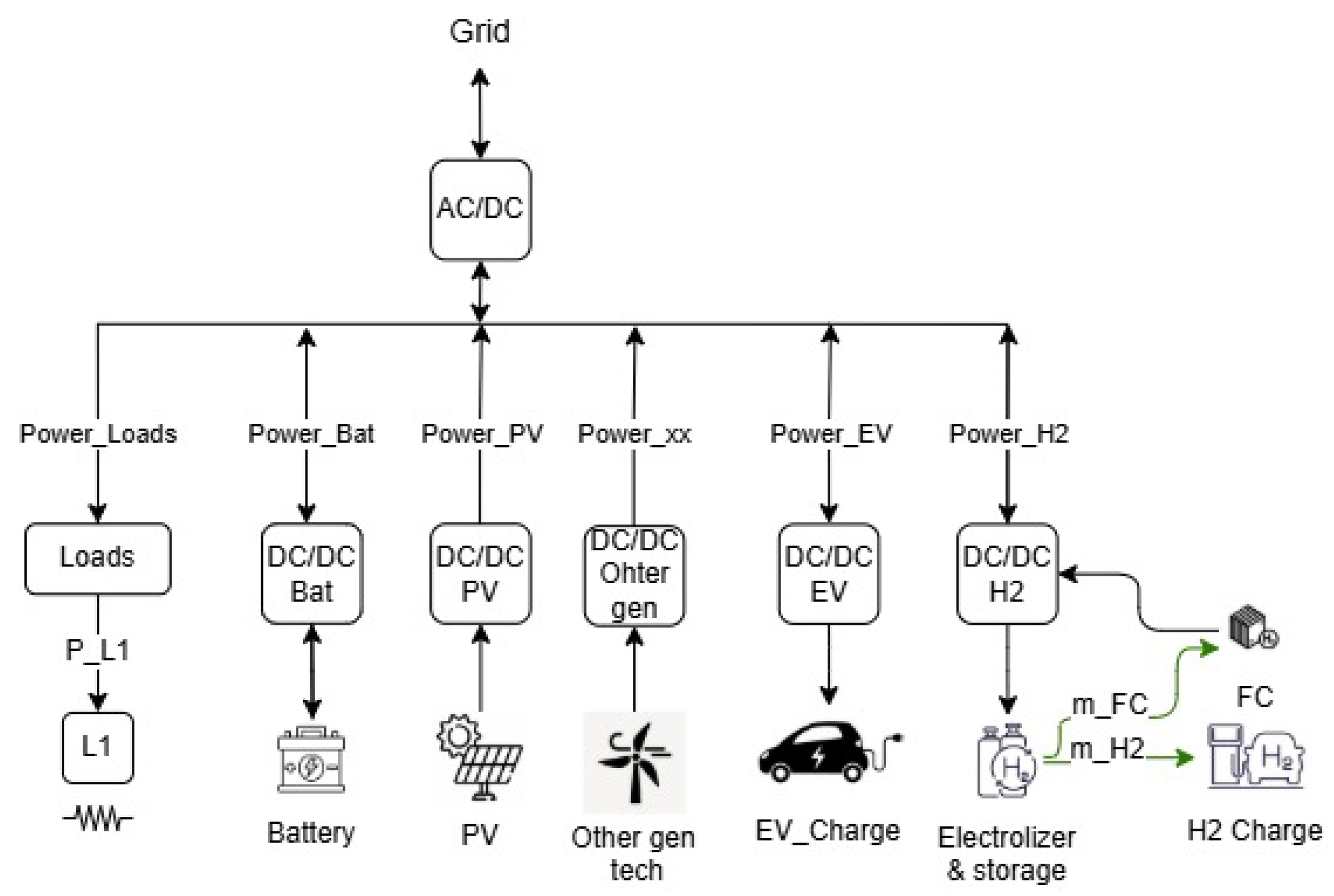
A detailed microgrid model has been developed, which includes solar photovoltaic systems for energy generation (in conjunction with alternative renewable energy sources such as wind and hydroelectric power), battery energy storage systems (BESS), electric vehicle (EV) charging infrastructures, hydrogen production facilities, and various energy consumption nodes, which can be classified as manageable and non-manageable (see Figure 6). This detailed microgrid model is customized to meet the specific installation requirements through the application of a configuration file that specifies the existing devices, along with the operational mode of the grid—whether interconnected or isolated—the incorporation of direct current (DC) or alternating current (AC) components, and additional operational factors, such as the ability to inject energy into the grid.
The fundamental operational parameters of the microgrid components (power output, storage capacity, efficiency, among others) are introduced through an auxiliary configuration file. Forecasts (such as solar generation, energy pricing, and energy demand) are introduced via a forecasts file, which has a considerable impact on the system’s results. This file further incorporates assessments of equipment availability, thereby facilitating the recalculation and establishment of optimal operational setpoints in alignment with the microgrid’s actual operational state.
Figure 6.
Example of a microgrid general model.
The objective function minimizes the total operating cost, which is the sum of component-wise terms associated with the battery, EV charging/V2G, hydrogen system, and grid exchanges. Battery and EV costs include an energy/usage term and a smoothing penalty that discourages highly irregular charging/discharging profiles. The hydrogen term accounts for electrolyser and fuel cell operation, optional auxiliary truck refilling, and hydrogen revenues from vehicle refuelling. In contrast, the grid term captures contracted power and time-dependent buy/sell transactions. Feasible operation is enforced through a DC-bus power balance (Kirchhoff-based) that includes converter efficiencies, PV utilisation limits bounded by forecasts and installed capacity, and asset-specific dynamics and limits. Storage devices (BESS, EV, and hydrogen tank) are constrained by initial state, minimum/maximum capacity, mutually exclusive charge/discharge modes, and inter-temporal state update equations; additional auxiliary variables model step-to-step power variations for smoothing. Finally, grid import/export is bounded by contracted power limits.
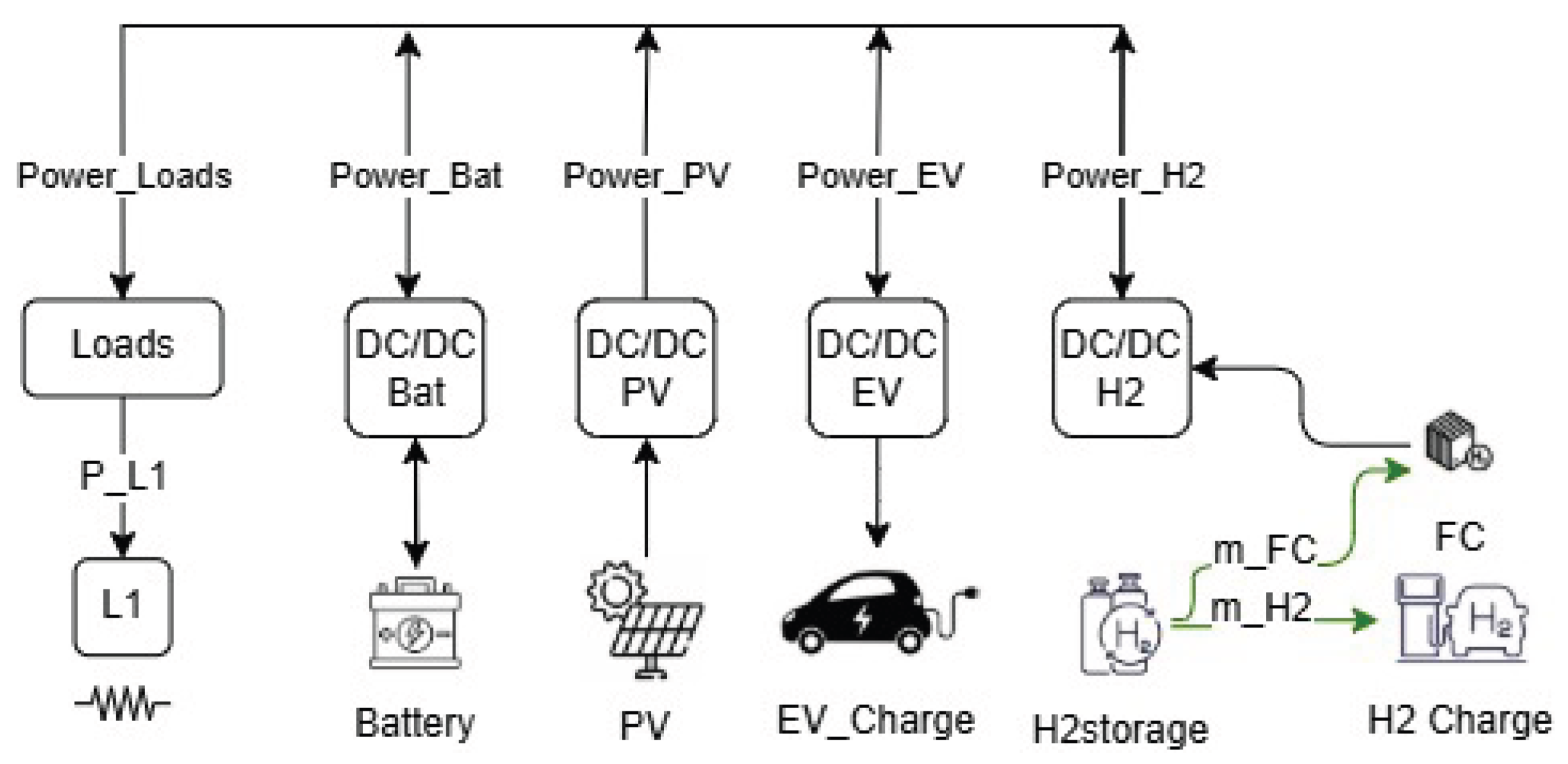
The general model presented in the previous paragraphs has been adapted to the characteristics of the use case examined in this paper, a real microgrid. The main characteristics are summarized in Table 4, and the microgrid schema is illustrated in Figure 7. The system operates independently of the electrical grid. It encompasses a photovoltaic solar generation system, a controllable electric vehicle charging station, a hydrogen refueling facility, and an energy storage system utilizing batteries. In this scenario, hydrogen is delivered to the system through external transport vehicles, given the absence of an electrolyzer. However, a fuel cell is incorporated to convert the stored hydrogen into electrical energy. The optimization model is also formulated to determine the appropriate timing for hydrogen imports.

Table 4.
Test site assets parameters.
| Asset | Parameter | Value |
|---|---|---|
| Test site microgrid | Grid connection | Isolated |
| Solar PV system | Rated power | 12 kW |
| Power range | 0–12 kW | |
| BESS | Technology | Lithium ion |
| Total Capacity | 53.9 kWh | |
| Minimum SoC | 10%, 5.39 kWh | |
| Max charging power | 26.6 kW | |
| Max discharging power | 53.9 kW | |
| Bus connection | Direct connection / no converter | |
| Estimated life | 5000 cycles | |
| Batt cost | 500 €/kWh | |
| EV charger | Rated power | 50 kW |
| Efficiency | 95% | |
| Hydrogen system/fuel cell | Max power | 100 kW |
| Min power | 10 kW | |
| Efficiency | 50–60% | |
| Hydrogen storage | Capacity | 41 kg 200 bar |
| Hydrogen system/electrolyser | No electrolyser | Hydrogen refuelling from external sources |
Figure 7.
The microgrid model used in the optimization process (reduction of the general schema in Figure 6).
Figure 7.
The microgrid model used in the optimization process (reduction of the general schema in Figure 6).
References
- Fang, X.; Misra, S.; Xue, G.; Yang, D. Smart Grid—The New and Improved Power Grid: A Survey. IEEE Communications Surveys & Tutorials 2012, 14, 944–980. [Google Scholar] [CrossRef]
- Staffell; Brett, D.; Brandon, N.; Hawkes, A. A review of domestic heat pumps. Energy & Environmental Science 2012, 5, 9291–9306. [Google Scholar] [CrossRef]
- Mejbaul Haque, M.; Wolfs, P. A review of high PV penetrations in LV distribution networks: Present status, impacts and mitigation measures. Renewable and Sustainable Energy Reviews 2016, 62, 1195–1208. [Google Scholar] [CrossRef]
- Shen, F.; Huang, S.; Wu, Q.; Repo, S.; Xu, Y.; Østergaard, J. Comprehensive Congestion Management for Distribution Networks based on Dynamic Tariff, Reconfiguration and Re-profiling Product. IEEE Transactions on Smart Grid 2019, 10, 4795–4805. [Google Scholar] [CrossRef]
- Lund, P. D.; Mikkola, J.; Salpakari, J.; Lindgren, J. Review of energy system flexibility measures to enable high levels of variable renewable electricity. Renewable and Sustainable Energy Reviews 2015, 45, 785–807. [Google Scholar] [CrossRef]
- Denholm, P.; Hand, M. Grid flexibility and storage required to achieve very high penetration of variable renewable electricity. Energy Policy 2011, 39, 1817–1830. [Google Scholar] [CrossRef]
- Palensky, P.; Dietrich, D. Demand Side Management: Demand Response, Intelligent Energy Systems, and Smart Loads. IEEE Transactions on Industrial Informatics 2011, 7, 381–388. [Google Scholar] [CrossRef]
- Meng, L.; Sanseverino, E. R.; Luna Hernandez, A. C.; Dragicevic, T.; Vasquez, J. C.; Guerrero, J. M. Microgrid supervisory controllers and energy management systems: A literature review. Renewable and Sustainable Energy Reviews 2016, 60, 1263–1273. [Google Scholar] [CrossRef]
- Parag, Y.; Sovacool, B. K. Electricity market design for the prosumer era. Nature Energy 2016, 1, 16032. [Google Scholar] [CrossRef]
- Parrish, B.; Heptonstall, P.; Gross, R.; Sovacool, B. K. A systematic review of motivations, enablers and barriers for consumer engagement with residential demand response. Energy Policy 2020, 138, 111221. [Google Scholar] [CrossRef]
- Fernández, G.; Hedar, A. S.; Torres, M.; Apostolidou, N.; Koltsaklis, N.; Spiliopoulos, N. System Requirements for Flexibility Markets Participation: A Stakeholder-Centric Survey from REEFLEX Project. Applied Sciences 2025, 15, 10426. [Google Scholar] [CrossRef]
- Afram; Janabi-Sharifi, F. Theory and applications of HVAC control systems—A review of model predictive control (MPC). Building and Environment 2014, 72, 343–355. [Google Scholar] [CrossRef]
- Parisio; Rikos, E.; Glielmo, L. A Model Predictive Control Approach to Microgrid Operation Optimization. IEEE Transactions on Control Systems Technology 2014, 22, 1813–1827. [Google Scholar] [CrossRef]
- Mayne, D. Q.; Rawlings, J. B.; Rao, C. V.; Scokaert, P. O. M. Constrained model predictive control: Stability and optimality. Automatica 2000, 36, 789–814. [Google Scholar] [CrossRef]
- Qin, S. J.; Badgwell, T. A. A survey of industrial model predictive control technology. Control Engineering Practice 2003, 11, 733–764. [Google Scholar] [CrossRef]
- Oldewurtel, F.; Parisio, A.; Jones, C. N.; Gyalistras, D.; Gwerder, M.; Stauch, V.; Lehmann, B.; Morari, M. Use of model predictive control and weather forecasts for energy efficient building climate control. Energy and Buildings 2012, 45, 15–27. [Google Scholar] [CrossRef]
- Hoffmann, M.; Kotzur, L.; Stolten, D.; Robinius, M. A Review on Time Series Aggregation Methods for Energy System Models. Energies 2020, 13, 641. [Google Scholar] [CrossRef]
- Hu, J.; Shan, Y.; Guerrero, J. M.; Ioinovici, A.; Chan, K. W.; Rodriguez, J. Model predictive control of microgrids—An overview. Renewable and Sustainable Energy Reviews 2021, 136, 110422. [Google Scholar] [CrossRef]
- Marquant, J. F.; Evins, R.; Carmeliet, J. Reducing Computation Time with a Rolling Horizon Approach Applied to a MILP Formulation of Multiple Urban Energy Hub System. Procedia Computer Science 2015, 51, 2137–2146. [Google Scholar] [CrossRef]
- Hönen, J.; Hurink, J. L.; Zwart, B. Dynamic Rolling Horizon-Based Robust Energy Management for Microgrids Under Uncertainty. arXiv 2023, arXiv:2307.05154. [Google Scholar] [CrossRef]
- Hoffmann, M.; Priesmann, J.; Nolting, L.; Praktiknjo, A.; Kotzur, L.; Stolten, D. Typical periods or typical time steps? A multi-model analysis to determine the optimal temporal aggregation for energy system models. Applied Energy 2021, 304, 117825. [Google Scholar] [CrossRef]
- Hoffmann, M.; Kotzur, L.; Stolten, D. The Pareto-optimal temporal aggregation of energy system models. Applied Energy 2022, 315, 119029. [Google Scholar] [CrossRef]
- Gao, Z.; Gazzani, M.; Tejada-Arango, D. A.; Siqueira, A. S.; Wang, N.; Gibescu, M.; Morales-España, G. Fully flexible temporal resolution for energy system optimization. Applied Energy 2025, 396, 126267. [Google Scholar] [CrossRef]
- Forough, Behzadi; Roshandel, R. Multi objective receding horizon optimization for optimal scheduling of hybrid renewable energy system. Energy and Buildings 2017, 150, 583–597. [Google Scholar] [CrossRef]
- Shin, S.; Zavala, V. M. Controllability and Observability Imply Exponential Decay of Sensitivity in Dynamic Optimization. IFAC-PapersOnLine 2021, 54, 179–184. [Google Scholar] [CrossRef]
- Shin, S.; Zavala, V. M. Diffusing-Horizon Model Predictive Control. IEEE Transactions on Automatic Control 2023, 68, 188–201. [Google Scholar] [CrossRef]
- Wang, Z.; Tao, H.; Cai, W.; Duan, Y.; Wu, D.; Zhang, L. Study on the multitime scale rolling optimization operation of a near-zero energy building energy supply system. Energy Conversion and Management 2022, 270, 116255. [Google Scholar] [CrossRef]
- Wei, S.; Gao, X.; Zhang, Y.; Li, Y.; Shen, J.; Li, Z. An improved stochastic model predictive control operation strategy of integrated energy system based on a single-layer multi-timescale framework. Energy 2021, 235, 121320. [Google Scholar] [CrossRef]
- Behrunani, V. N.; Cai, H.; Heer, P.; Smith, R. S.; Lygeros, J. Distributed multi-horizon model predictive control for network of energy hubs. Control Engineering Practice 2024, 147, 105922. [Google Scholar] [CrossRef]
- Abdulla, K.; De Hoog, J.; Steer, K.; Wirth, A.; Halgamuge, S. Multi-Resolution Dynamic Programming for the Receding Horizon Control of Energy Storage. IEEE Transactions on Sustainable Energy 2019, 10, 333–343. [Google Scholar] [CrossRef]
- Yu, Z.; Zhong, H.; Ruan, G.; Yan, X. Network-Constrained Unit Commitment With Flexible Temporal Resolution. IEEE Transactions on Power Systems 2024. [Google Scholar] [CrossRef]
- Tao, J.; Li, R.; Pineda, S. Unit Commitment with Cost-Oriented Temporal Resolution. arXiv 2025, arXiv:2506.02707. [Google Scholar] [CrossRef]
- Marcy; Goforth, T.; Nock, D.; Brown, M. Comparison of temporal resolution selection approaches in energy systems models. Energy 2022, 251, 123969. [Google Scholar] [CrossRef]
- Mishra, M. K.; Parida, S. K. A Game Theoretic Horizon Decomposition Approach for Real-Time Demand-Side Management. IEEE Transactions on Smart Grid 2022, 13, 3532–3545. [Google Scholar] [CrossRef]
- Aguilar; Quinones, J.; Pineda, L.; Ostanek, J.; Castillo, L. Optimal scheduling of renewable energy microgrids: A robust multi-objective approach with machine learning-based probabilistic forecasting. Applied Energy 2024, 369, 123548. [Google Scholar] [CrossRef]
Figure 1.
Examples of uniform and fully flexible temporal resolutions from [23].
Figure 1.
Examples of uniform and fully flexible temporal resolutions from [23].
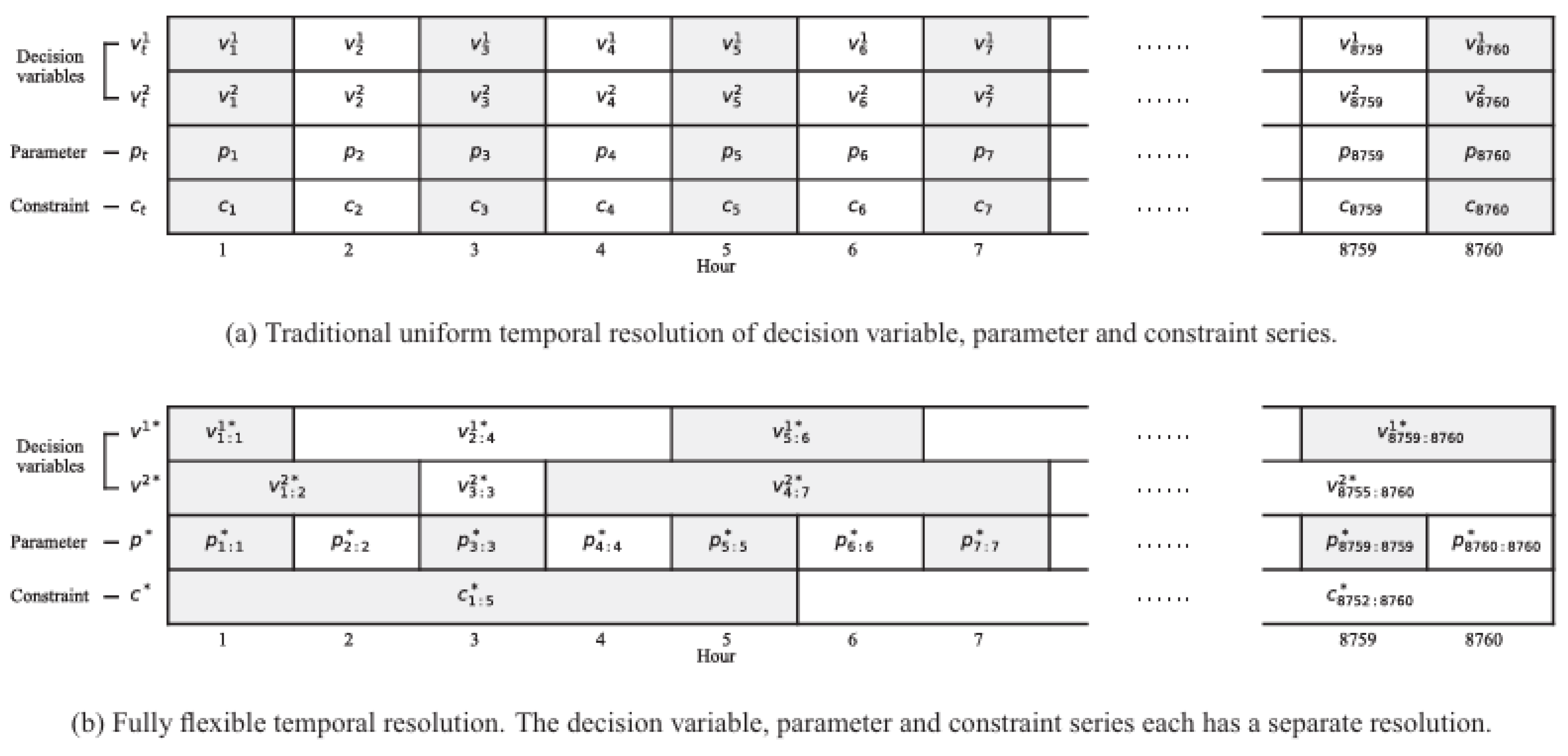
Figure 2.
Overview of the proposed compute-aware workflow to select an EMS/MPC optimization horizon and a block-variable temporal granularity.
Figure 2.
Overview of the proposed compute-aware workflow to select an EMS/MPC optimization horizon and a block-variable temporal granularity.
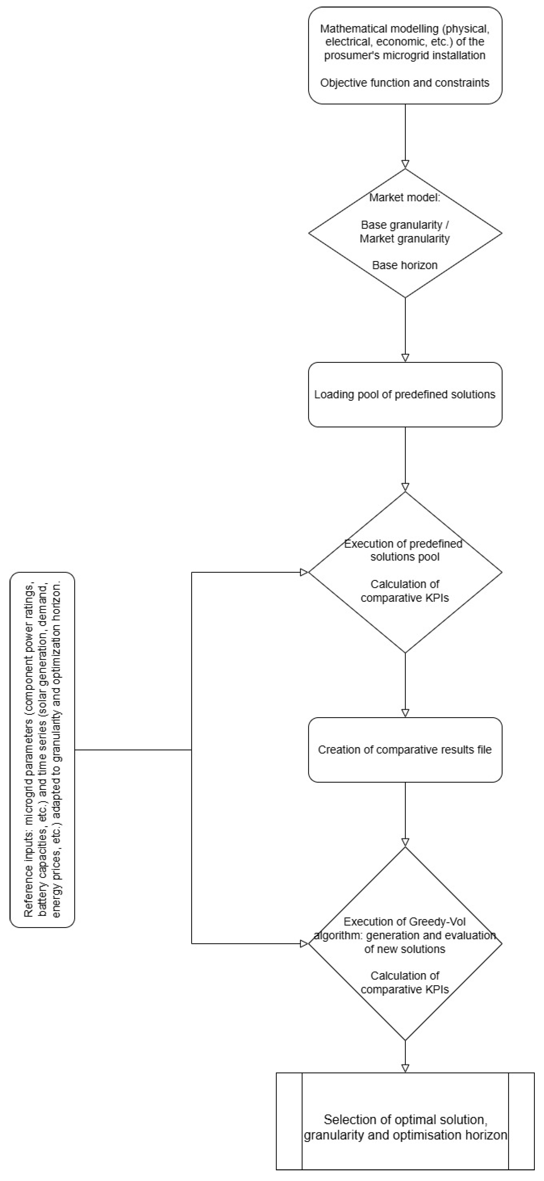
Figure 3.
Predefined pool of solutions evaluation for 1-hour market, optimization results vs execution time.
Figure 3.
Predefined pool of solutions evaluation for 1-hour market, optimization results vs execution time.
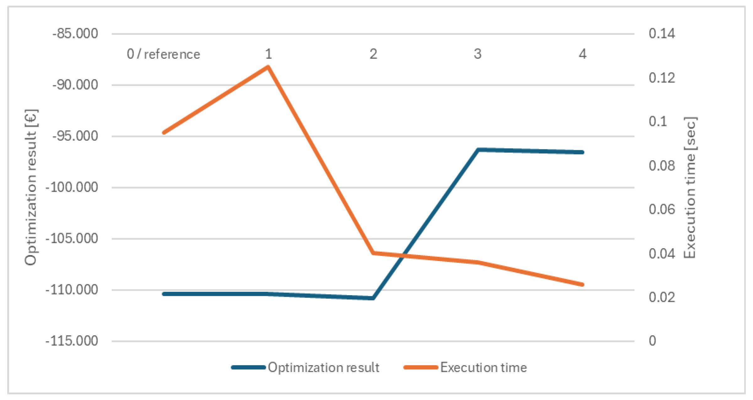
Figure 4.
Predefined pool of solutions evaluation for 1-hour market, execution time vs solution steps.
Figure 4.
Predefined pool of solutions evaluation for 1-hour market, execution time vs solution steps.
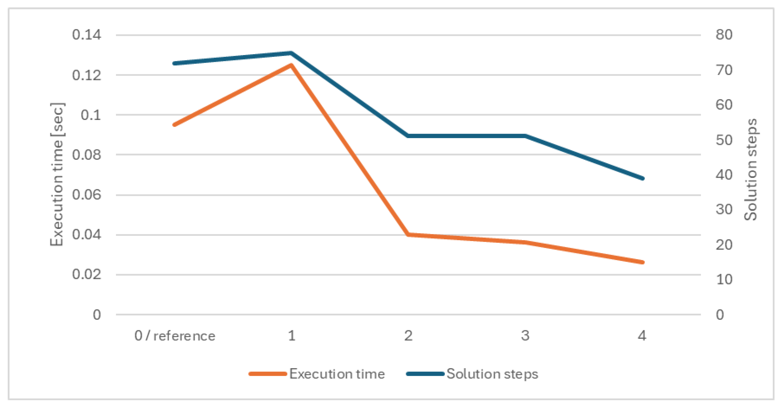
Figure 5.
Results of applying the Greedy-VoI algorithm without the restriction of equation (10) and without maximum block limits.
Figure 5.
Results of applying the Greedy-VoI algorithm without the restriction of equation (10) and without maximum block limits.
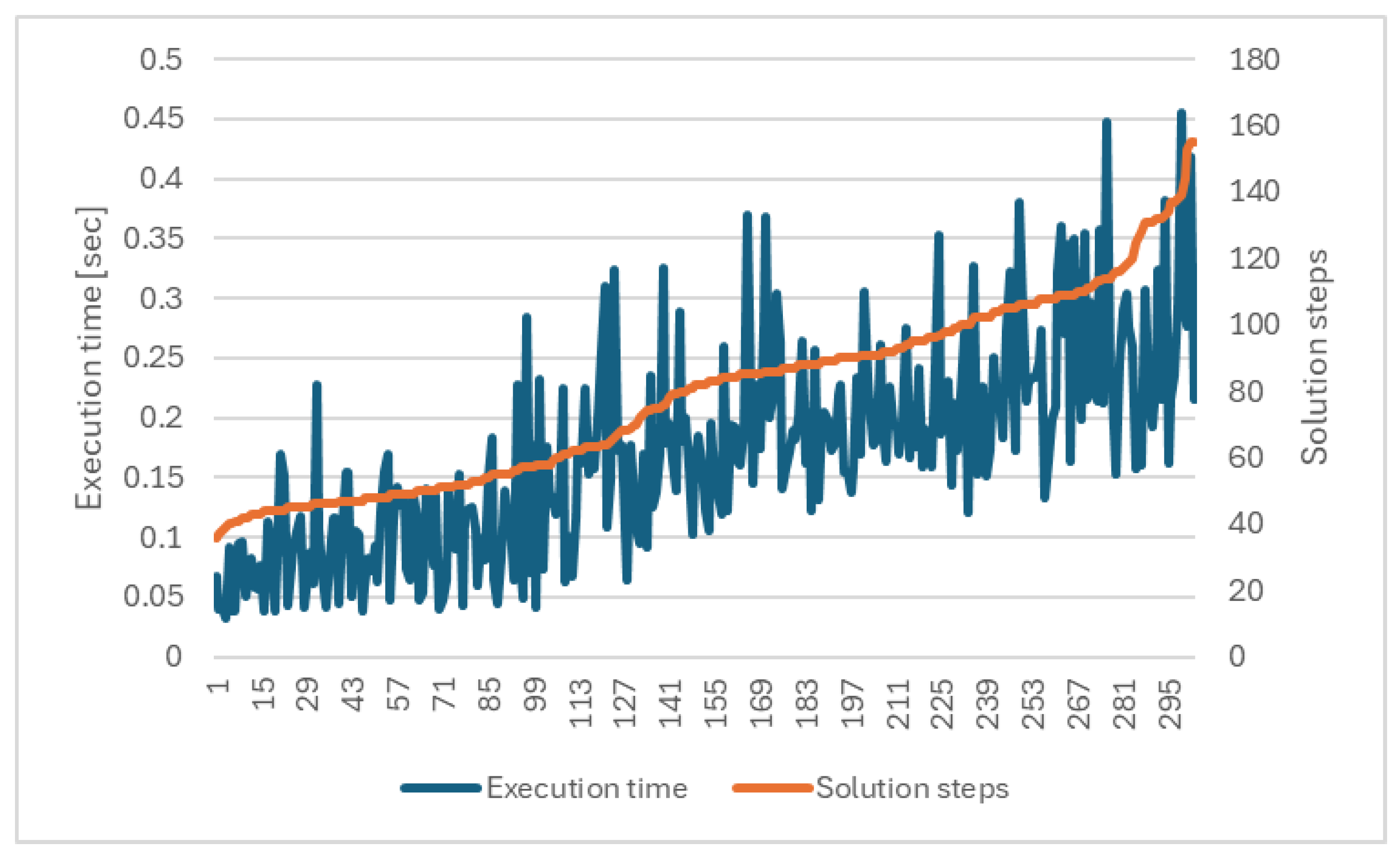
Table 1.
Mathematical definition of a predefined pool of solutions.
| Market step |
Solution | H [horizon] | i [blocks] | n1 | Δt1 | n2 | Δt2 | n3 | Δt3 | [(n1xΔt)…(nBxΔtB);H] |
|---|---|---|---|---|---|---|---|---|---|---|
| 1 hour | 0 / reference | 3 days 72 hours 4320 minutes |
1 | 72 | 60 | [(72x60); 4320] | ||||
| 1 | 3 days 72 hours 4320 minutes |
2 | 4 | 15 | 71 | 60 | [(4x15),(71x60); 4320] | |||
| 2 | 3 days 72 hours 4320 minutes |
3 | 4 | 15 | 23 | 60 | 24 | 120 | [(4x15),(23x60),(24x120); 4320] | |
| 3 | 2 days 48 hours 2880 minutes |
2 | 4 | 15 | 47 | 60 | [(4x15),(47x60); 2880] | |||
| 4 | 2 days 48 hours 2880 minutes |
3 | 4 | 15 | 23 | 60 | 12 | 120 | [(4x15),(23x60),(12x120); 2880] | |
| 15 minutes | 0 / reference | 3 days 72 hours 4320 minutes |
1 | 288 | 15 | [(288x15); 4320] | ||||
| 1 | 3 days 72 hours 4320 minutes |
2 | 3 | 5 | 287 | 15 | [(3x5),(287x15); 4320] | |||
| 2 | 3 days 72 hours 4320 minutes |
3 | 3 | 5 | 95 | 15 | 48 | 60 | [(3x5),(95x15),(48,60); 4320] | |
| 3 | 2 days 48 hours 2880 minutes |
2 | 3 | 5 | 191 | 15 | [(3x5),(191x15); 2880] | |||
| 4 | 2 days 48 hours 2880 minutes |
3 | 3 | 5 | 95 | 15 | 24 | 60 | [(3x5),(95x15),(24x60); 2880] |
Table 2.
Predefined pool of solutions evaluation for a 1-hour market.
| Market step |
H [horizon] | Solution | n1 | Δt1 | n2 | Δt2 | n3 | Δt3 | [(n1,Δt)…(nB,ΔtB);H] | Optimization result [€] |
Execution Time [sec] |
|---|---|---|---|---|---|---|---|---|---|---|---|
| 1 hour | 3 days 72 hours 4320 minutes |
0 / reference | 72 | 60 | [(72x60); 4320] | -110.386 | 0.095 | ||||
| 3 days 72 hours 4320 minutes |
1 | 4 | 15 | 71 | 60 | [(4x15),(71x60); 4320] | -110.386 | 0.125 | |||
| 3 days 72 hours 4320 minutes |
2 | 4 | 15 | 23 | 60 | 24 | 120 | [(4x15),(23x60),(24x120); 4320] | -110.793 | 0.04 | |
| 2 days 48 hours 2880 minutes |
3 | 4 | 15 | 47 | 60 | [(4x15),(47x60); 2880] | -96.318 | 0.036 | |||
| 2 days 48 hours 2880 minutes |
4 | 4 | 15 | 23 | 60 | 12 | 120 | [(4x15),(23x60),(12x120); 2880] | -96.563 | 0.026 |
Table 3.
Predefined pool of solutions evaluation for a 15-minute market.
| Market step |
H [horizon] | Solution | n1 | Δt1 | n2 | Δt2 | n3 | Δt3 | [(n1xΔt)…(nBxΔtB);H] | Optimization result [€] |
Execution Time [sec] |
|---|---|---|---|---|---|---|---|---|---|---|---|
| 15 minutes | 3 days 72 hours 4320 minutes |
0 / reference | 288 | 15 | [(288x15); 4320] | -99.596 | 1.06 | ||||
| 3 days 72 hours 4320 minutes |
1 | 3 | 5 | 287 | 15 | [(3x5),(287x15); 4320] | -99.596 | 1.264 | |||
| 3 days 72 hours 4320 minutes |
2 | 3 | 5 | 95 | 15 | 48 | 60 | [(3x5),(95x15),(48,60); 4320] | -110.424 | 0.666 | |
| 2 days 48 hours 2880 minutes |
3 | 3 | 5 | 191 | 15 | [(3x5),(191x15); 2880] | -57.200 | 0.289 | |||
| 2 days 48 hours 2880 minutes |
4 | 3 | 5 | 95 | 15 | 24 | 60 | [(3x5),(95x15),(24x60); 2880] | -70.96 | 0.189 |
Disclaimer/Publisher’s Note: The statements, opinions and data contained in all publications are solely those of the individual author(s) and contributor(s) and not of MDPI and/or the editor(s). MDPI and/or the editor(s) disclaim responsibility for any injury to people or property resulting from any ideas, methods, instructions or products referred to in the content. |
© 2025 by the authors. Licensee MDPI, Basel, Switzerland. This article is an open access article distributed under the terms and conditions of the Creative Commons Attribution (CC BY) license (http://creativecommons.org/licenses/by/4.0/).
Copyright: This open access article is published under a Creative Commons CC BY 4.0 license, which permit the free download, distribution, and reuse, provided that the author and preprint are cited in any reuse.


