Submitted:
24 December 2025
Posted:
26 December 2025
You are already at the latest version
Abstract
The paper proposes single-layer neural network algorithms for solving ordinary differential equations of the second order, built on the principles of functional link. According to this principle, the hidden layer of the neural network is replaced by a functional expansion block to improve input patterns using orthogonal Chebyshev, Legendre and Laguerre polynomials. The algorithms of polynomial neural networks were implemented in the Python programming language in the PyCharm environment. The operation of the algorithms of polynomial neural networks was tested by solving the initial and boundary value problems for the nonlinear Lane-Emden equation. The results of the solution are compared with the exact solution of the problems under consideration, as well as with the solution obtained using a multilayer perceptron. It is shown that polynomial neural networks can work more efficiently than multilayer neural networks. The issues of overfiting of polynomial neural networks and scenarios for overcoming it are considered.
Keywords:
algorithms
; orthogonal polynomials
; multilayer perceptron
; differential equations
; Cauchy problem
; boundary value problem
; overfitting
MSC: 34A34; 33C45; 68T05
1. Introduction
In recent years, machine learning methods, particularly artificial neural networks (ANNs), have found widespread application beyond traditional data analysis tasks, entering the realm of scientific computing [1]. One promising direction is the use of ANNs for the numerical solution of differential equations, opening new possibilities for modeling complex physical and engineering systems [2]. Compared to classical numerical methods (such as the finite difference or finite element method), neural network approaches offer several potential advantages: they allow obtaining a solution in the form of a continuous and differentiable function over the entire domain, can work efficiently in high-dimensional spaces, and are well-suited for problems with inverse parameters or incomplete data.
Various neural network architectures are used to solve ordinary differential equations (ODEs). The most common are multilayer networks, such as the classic multilayer perceptron (MLP) [3] or specialized Physics-Informed Neural Networks (PINNs), which explicitly incorporate governing laws into the loss function [4]. However, these architectures often require significant computational resources for training due to the large number of tunable parameters and can suffer from the vanishing gradient problem. An alternative is offered by single-layer neural networks based on the functional link principle (Functional Link Artificial Neural Network, FLANN) [6]. In the FLANN model, the hidden layer is replaced by a functional expansion block that increases the dimensionality of the input data through decomposition into orthogonal polynomial bases (e.g., Chebyshev, Legendre). This significantly reduces the number of network parameters and the number of iterations required for convergence, making FLANN a computationally efficient model with a high training speed.
FLANN networks based on Chebyshev (ChNN) and Legendre (LeNN) polynomials have already been successfully applied to solve various ODEs [7,8,9], demonstrating competitive accuracy. However, the literature lacks a systematic investigation and direct comparison of the effectiveness of these two approaches. Moreover, the potential of neural networks based on other classical orthogonal polynomials, particularly Laguerre polynomials (LaNN), for solving initial and boundary value problems for ODEs remains virtually unexplored. Thus, there is a clear knowledge gap: there is no comparative analysis within the entire family of polynomial FLANNs, nor an assessment of their advantages compared to standard deep architectures.
The aim of this work is to fill this gap through a comprehensive study of the performance of the family of single-layer polynomial neural networks ChNN, LeNN, and LaNN. The Cauchy problem and the boundary value problem for a nonlinear second-order ODE of the Lane-Emden type, for which an exact analytical solution is known, are chosen as test examples. This allows for an objective assessment of the accuracy of each method. The paper conducts a comparative analysis of the polynomial networks among themselves, as well as with the reference multilayer neural network MLP, based on two key criteria: the accuracy of the solution approximation and the algorithm execution time. It is demonstrated that properly configured polynomial networks can outperform MLP in computational efficiency while maintaining high accuracy, making them a promising tool for rapid numerical integration of differential equations.
2. Preliminaries
Orthogonal polynomials are widely used in approximation theory, in particular for constructing quadrature formulas for approximate calculation of integrals or function approximation [10].
Let and be real functions belonging to the class .
Definition 1.
Legendre polynomials of degree n for form an orthogonal system and can be computed by the recurrence formula:
Definition 2.
Chebyshev polynomials of degree n for form an orthogonal system and can be computed by the recurrence formula:
Definition 3.
Laguerre polynomials of degree n for form an orthogonal system and can be computed by the recurrence formula:
3. Neural Network Model Based on Orthogonal Polynomials
Consider a single-layer neural network based on the functional-link principle (Figure 1).
Figure 1 shows the structure of a single-layer neural network, which consists of one input node, one output layer and a functional expansion block based on Legendre, Chebyshev and Laguerre orthogonal polynomials. Here, by the notation OPNN we will mean one of the three neural networks LeNN, LaNN or ChNN. The hidden layer is eliminated by transforming the input pattern into a higher-dimensional space using polynomials (1)-(3).
As input data, we consider a vector of dimension n. The enhanced pattern is obtained using orthogonal polynomials (1)-(3):
According to (4), n-dimensional input x is extended into m-dimensional improved polynomials. Then a weighted sum z of the expanded input data is formed, which is written as:
To update the weights of the neural network, the error backpropagation learning algorithm is used. Thus, the gradient of the error function with respect to the tunable parameters is determined. The nonlinear hyperbolic tangent function is considered as the activation function. For training, the gradient descent algorithm is used, and the weights are updated using the negative gradient at each iteration. The weights are initialized randomly and then updated:
where is the learning parameter taking values from 0 to 1, k is the iteration step used to update the weights, as usual in neural networks, and is the error function, .
The output layer is determined by the input vector x and the tunable parameters of the selected neural network by the formula:
The activation function (7) can be chosen differently depending on the problem.
4. Problem Statement
Consider the following problem for a second order ODE for :
Problem (8) is a Cauchy problem.
Definition 4.
The trial solution of the Cauchy problem (8) we will call the function:
Consider the following boundary value problem for a second order ODE for :
Definition 5.
The trial solution of the boundary value problem (10) we will call the function:
5. Algorithms for Implementing Polynomial Neural Networks
The polynomial neural network algorithms were implemented in the Python programming language [11] in the PyCharm environment [12] in the OPNN computer program. The OPNN program flowchart is shown in Figure 2. It consists of two stages: the first stage defines the input parameters and selects the appropriate polynomial neural network, while the second stage contains the procedures for training it and inferring the obtained results. The main procedures in the algorithms are presented as pseudocode (Algorithms 1-7).
Note that Algorithms 1-5 are the same for the Cauchy problem and the boundary value problem, but the differences lie in the definition of the trial function (9) and (11), i.e., Algorithms 6 and 7.
| Algorithm 1 Neural Network Training for ODE Solution |
|
| Algorithm 2 Model Training Procedure |
|
| Algorithm 3 Loss Function Computation |
|
| Algorithm 4 Trial Solution Derivative Computation |
|
| Algorithm 5 Polynomial Neural Network Forward Pass |
|
PolynomialBasis(x) is a procedure for calculating a polynomial basis for a given input x. Depending on the type of neural network, it invokes different procedures according to definitions (1)-(3).
A trial solution to the Cauchy problem according to formula (9) is calculated using Algorithm 6.
| Algorithm 6 Trial Solution with Boundary Conditions (The Cauchy Problem) |
|
A trial solution to the boundary value problem according to formula (11) is calculated using Algorithm 7.
| Algorithm 7 Trial Solution with Boundary Conditions (Boundary value problem) |
|
6. Research Results
Consider the operation of orthogonal polynomial networks on the example of solving the Cauchy problem for the singular nonlinear Lane-Emden differential equation:
as well as for the boundary value problem:
Remark 1.
Remark 2.
Based on Definition 4 by formula (9), the trial solution for the Cauchy problem (13) is written as:
and for the boundary value problem (14), also valid is the exact solution (15) and taking into account representation (11) in the form:
The parameters of the orthogonal polynomial neural networks were set as follows: order of polynomials , number of training points 11 from the segment , number of epochs 10000, learning rate . The calculation results for solving the Cauchy problem (13) are given in Table 1.
From Table 1 it can be seen that the polynomial neural networks give approximately the same result. Figure 3 shows the solution graph obtained by the LaNN neural network, and Figure 4 shows the loss graph during training.
The graph in Figure 3 demonstrates the efficiency of the Laguerre NN neural network in solving the Cauchy problem (13). The loss function graph on a logarithmic scale is shown in Figure 4.
From Figure 4 it can be seen that the loss decreases with an increase in the number of epochs, which indicates successful model training. At the beginning of training (first 200 epochs), a rapid decrease in loss is observed, then the rate of decrease slows down, which is typical for the neural network training process.
The loss graph allows adjusting the hyperparameters of the neural network: learning rate, number of epochs, etc.
Here it can be noted that the LaNN neural network solved the problem more accurately than the ChNN network, but was less accurate than the LeNN network.
Table 3 shows the work of the multilayer neural network MLP with two hidden layers of 20 and 40 neurons respectively for solving the Cauchy problem (13).
It can be seen from Table 3 that to achieve acceptable accuracy in MLP, it is necessary to increase the number of neurons in each layer. This leads, as we will show below, to an increase in the algorithm execution time.
From Table 4 it can be seen that increasing the number of neurons in each hidden layer leads to a deterioration in the accuracy of solving the boundary value problem (14). Let us show how the execution time of algorithms for solving problems (13) and (14) depends on the choice of neural network architecture. Neural network parameters: learning rate , number of epochs – 1000, order of polynomials .
From Table 5 it can be seen that . Here it should be noted that the neural network based on Laguerre orthogonal polynomials coped with the task faster than the neural network based on Legendre orthogonal polynomials. Moreover, the LaNN and ChNN neural networks were faster in solving the Cauchy problem (13) than the multilayer MLP network.
From Table 6 it follows that , and therefore the trend in the execution times of algorithms for solving the boundary value problem (14) remains as in Table 5. Here, a multilayer neural network MLP with three hidden layers of 20 neurons in each layer was used. From Table 6 it follows that single-layer orthogonal polynomial neural networks can work faster than multilayer neural networks of the MLP type, for example, the LeNN neural network.
It should be noted that increasing the order of the polynomial n can also lead to a deterioration in the result. Let us take the parameters for the LeNN neural network from the previous example (Table 3) and find solutions to problems (13) and (14) for polynomial orders and . The research results are given in Table 7 and Table 8.
From Table 7 we see that with an increase in the order of the polynomial, the calculation error increased, although the algorithm execution time decreased from 10.01 s for to 8.92 s for .
7. Overfitting Issues
It should be noted that the issue of overfitting remains relevant when using neural networks to solve differential equations. Overfitting here in the context of the problem of solving a differential equation is understood differently. Here, the training sample is the differential equation itself, which essentially defines an infinite set of constraints that the solution function must satisfy. The neural network here tries to approximate this function that satisfies these constraints everywhere in a given domain. It should also be said that there is no division of data into test and training samples here. We are looking for a single solution for the entire domain. The concept of "new data" from the same domain is erased — we want the network to work well on the entire domain at once. Thus, pure "memorization of noise in the training data" is not applicable here, since there are no discrete data initially. The concept of overfitting is understood mainly as overfitting at collocation points. We cannot check the fulfillment of the equation on the entire infinite domain. Therefore, we choose a finite set of points (collocation points) at which we calculate the residual of the equation and minimize it. The neural network between collocation points can behave incorrectly, for example, oscillate. The residual at the training collocation points will be very low (sometimes almost zero), but if we check the solution on another, denser grid of points, the residual will be huge. This is a sign of overfitting. Similarly, the concept of overfitting can arise at boundary (initial) points of the domain.
Here, overfitting can be combated by various methods similar to solving the issue of classical overfitting. For example, known methods are L1/L2 regularization, adaptive weights for the loss function, etc. However, in our opinion, the most effective and common method is dynamic selection of collocation points. Instead of using a fixed set of points, at each iteration (or after several epochs) collocations are selected anew (often randomly). Here it is necessary to remember about the non-optimal choice of collocation points. If the points at which the equation residual is calculated are chosen unsuccessfully (for example, uniformly over the entire domain), the network may learn well in some areas and poorly in others (for example, in areas of high gradients) [14]. This approach does not allow the network to "memorize" their location and forces it to learn to satisfy the equation in the entire domain. We also note article [4], in which the authors study the issues of overfitting of the multilayer PINN caused by gradient imbalance.
8. Conclusions
The work for the first time investigated the approximate solution of the Cauchy problem and the boundary value problem for the Lane-Emden differential equation using three single-layer neural networks based on Legendre, Chebyshev and Laguerre orthogonal polynomials. It is shown that the new neural network based on Laguerre polynomials gives acceptable results, and in some cases can be more accurate than the ChNN neural network and faster than the LeNN neural network. All three polynomial neural networks were also compared with the multilayer MLP neural network. Research has shown that single-layer polynomial neural networks can work better than the multilayer MLP neural network. Key parameters for polynomial neural networks, in addition to choosing the number of training epochs and learning rate, is the order of the polynomial. However, this order must be chosen optimally; its further increase or decrease can lead to a deterioration in results. Note that in multilayer neural networks it is necessary to adjust the number of hidden layers and the number of neurons in each of them. The latter means that single-layer polynomial neural networks have a simpler architecture than multilayer neural networks and, accordingly, they are easier to implement on a computer. The choice of neural network architecture depends on the specific task for an ordinary differential equation.
Funding
The work was carried out within the framework of the state assignment of IKIR FEB RAS (reg. No. 124012300245-2).
Data Availability Statement
The original contributions presented in this study are included in the article. Further inquiries can be directed to the corresponding author.
Abbreviations
The following abbreviations are used in this manuscript:
| ChNN | Chebyshev Neural Network |
| FLANN | Functional Link Artificial Neural Network |
| LeNN | Legendre Neural Network |
| LaNN | Laguerre Neural Network |
| MLP | Multilayer Perceptron |
| PINN | Physics-Informed Neural Networks |
References
- Abdolrasol, M.G.M.; Hussain, S.M.S.; Ustun, T.S.; Sarker, M.R.; Hannan, M.A.; Mohamed, R.; Ali, J.A.; Mekhilef, S.; Milad, A. Artificial Neural Networks Based Optimization Techniques: A Review. Journal Abbreviation 2021, 10, 2689. [Google Scholar] [CrossRef]
- Tan, L. S.; Zainuddin, Z.; Ong, P. Solving ordinary differential equations using neural networks. AIP Conference Proceedings 2018, 1974, 020070. [Google Scholar] [CrossRef]
- Riedmiller, M.; Lernen, A. Multi layer perceptron. Machine learning lab special lecture, University of Freiburg 2014, 24, 11-60.
- Wang, S.; Teng, Y.; Perdikaris, P. Understanding and mitigating gradient flow pathologies in physics-informed neural networks. SIAM Journal on Scientific Computing 2021, 43, A3055–A3081. [Google Scholar] [CrossRef]
- Fan, Q.; Zhang, X.; Wen, Z.; Xu, L.; Zhang, Q. Nonlinear Compensation of the Linear Variable Differential Transducer Using an Advanced Snake Optimization Integrated with Tangential Functional Link Artificial Neural Network. Sensors 2025, 25, 1074. [Google Scholar] [CrossRef] [PubMed]
- Pao, Y.H.; Phillips, S.M. The functional link net and learning optimal control. Neurocomputing 1995, 9, 149–164. [Google Scholar] [CrossRef]
- Chaharborj, S. S.; Chaharborj, S. S.; See, P. P. Application of Chebyshev neural network to solve Van der Pol equations. International Journal of Basic and Applied Sciences 2021, 10, 7–19. [Google Scholar] [CrossRef]
- Mall, S.; Chakraverty, S. Application of Legendre neural network for solving ordinary differential equations. Applied Soft Computing 2016, 43, 347–356. [Google Scholar] [CrossRef]
- Yang, Y.; Hou, M.; Luo, J. A novel improved extreme learning machine algorithm in solving ordinary differential equations by Legendre neural network methods. Advances in Difference Equations 2018, 2018, 469. [Google Scholar] [CrossRef]
- Chihara, T. S. An introduction to orthogonal polynomials; Courier Corporation: Mineola, USA, 2011. [Google Scholar]
- Shaw, Z.A. Learn Python the Hard Way; Addison-Wesley Professional: Boston, USA, 2024. [Google Scholar]
- Van Horn, B. M.; Nguyen, Q. Hands-on application development with PyCharm: Build applications like a Pro with the ultimate Python development tool; Packt Publishing Ltd: Bermingham, UK, 2023. [Google Scholar]
- Yildirim, A.; Ozis, T. Solutions of singular IVPs of Lane–Emden type by the variational iteration method. Nonlinear Anal. 2009, 70, 2480–2484. [Google Scholar] [CrossRef]
- Nabian, M. A.; Gladstone, R. J.; Meidani, H. Efficient training of physics-informed neural networks via importance sampling. Computer-Aided Civil and Infrastructure Engineering 2021, 36, 962–977. [Google Scholar] [CrossRef]
- Mall, S.; Chakraverty, S. Single layer Chebyshev neural network model for solving elliptic partial differential equations. Neural Processing Letters 2017, 45, 825–840. [Google Scholar] [CrossRef]
- Tverdyi, D.; Parovik, R. Application of the Fractional Riccati Equation for Mathematical Modeling of Dynamic Processes with Saturation and Memory Effect. Fractal and Fractional 2022, 6, 163. [Google Scholar] [CrossRef]
- Allahviranloo, T.; Jafarian, A.; Saneifard, R.; Ghalami, N.; Nia; Measoomy, S.; Kiani, F.; Fernandez-Gamiz, U.; Noeiaghdam, S. An application of artificial neural networks for solving fractional higher-order linear integro-differential equations. Bound. Value Probl. 2023, 2023, 74. [Google Scholar] [CrossRef]
- Tverdiy, D. A.; Makarov, E.O.; Parovik, R.I. Hereditary Mathematical Model of the Dynamics of Radon Accumulation in the Accumulation Chamber. Mathematics 2023, 11, 850. [Google Scholar] [CrossRef]
- Nguyen, T. D. Neural network method for solving the boundary value problem for fractional differential equations. Computational methods and programming 2025, 26, 245–253. [Google Scholar]
- Ali, I. Advanced machine learning technique for solving elliptic partial differential equations using Legendre spectral neural networks. Electronic Research Archive 2025, 33, 826–848. [Google Scholar] [CrossRef]
Figure 1.
Structure of a single-layer neural network based on orthogonal polynomials.
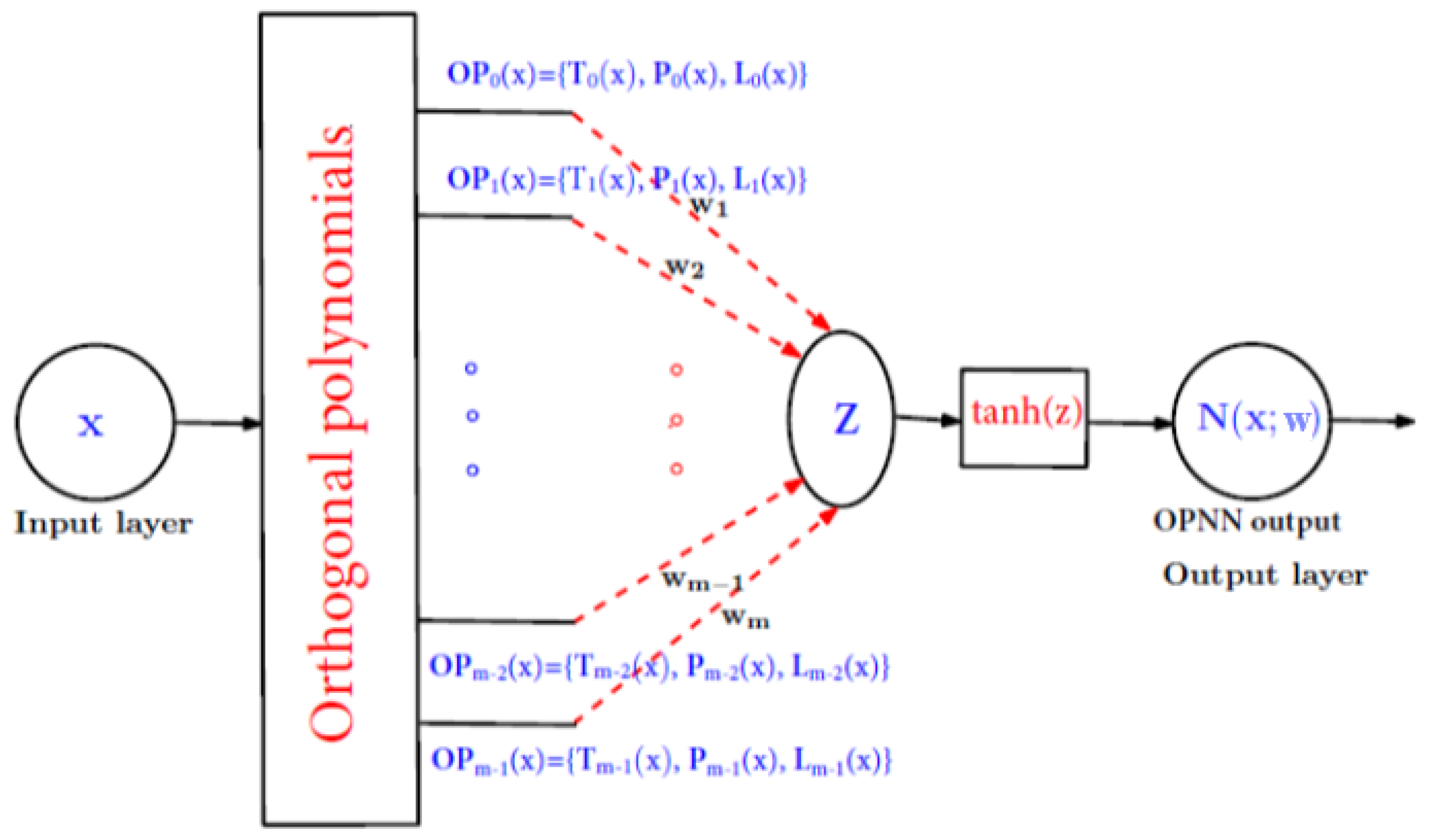
Figure 2.
(a) – Stage 1: data input and neural network initialization; (b) – Stage 2: training and output of simulation results.
Figure 2.
(a) – Stage 1: data input and neural network initialization; (b) – Stage 2: training and output of simulation results.
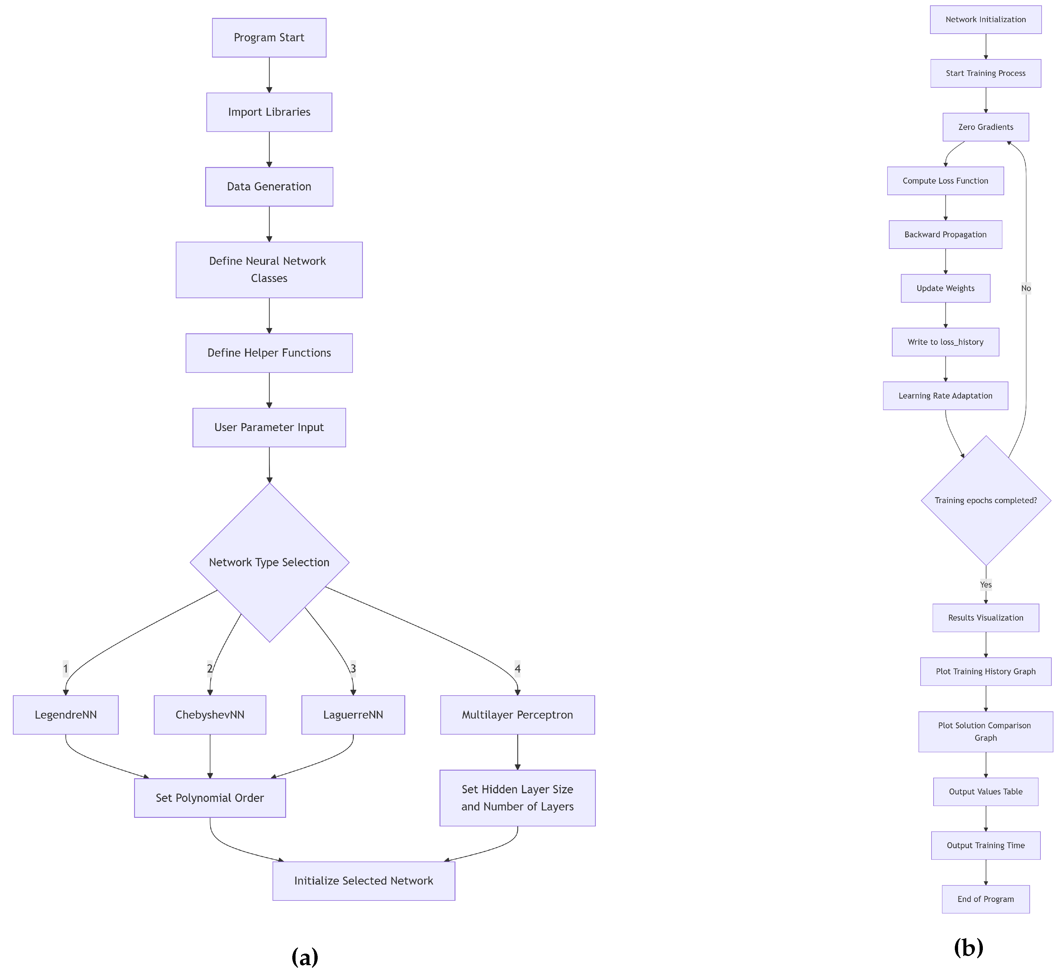
Figure 3.
Example of LaNN neural network operation.
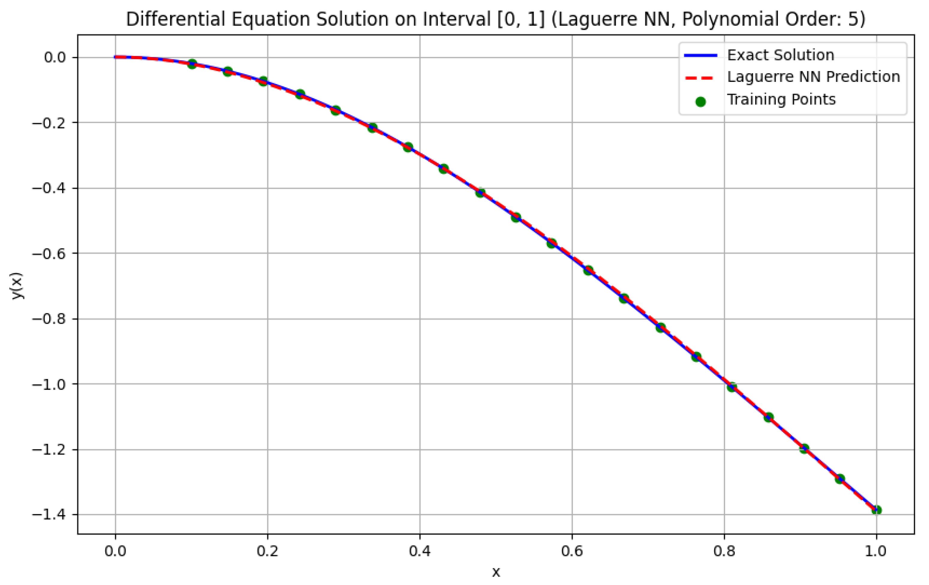
Figure 4.
Loss graph during training with LaNN neural network.
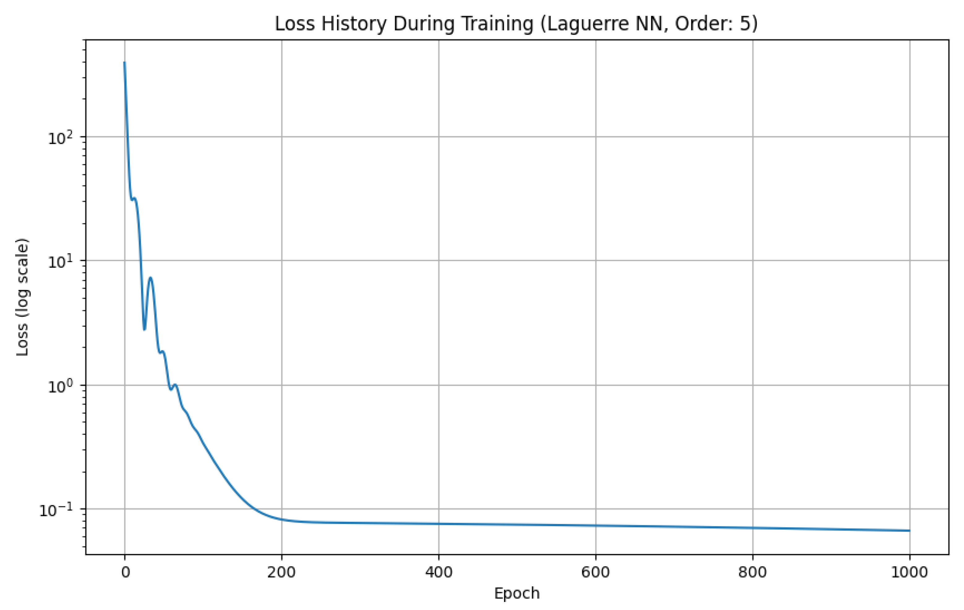

Table 1.
Solution of the Cauchy problem (13) using polynomial neural networks ().
Table 1.
Solution of the Cauchy problem (13) using polynomial neural networks ().
| x | Exact | LeNN | Err | ChNN | Err | LaNN | Err |
|---|---|---|---|---|---|---|---|
| 0.0 | 0.000000 | 0.000000 | 0.000000 | 0.000000 | 0.000000 | 0.000000 | 0.000000 |
| 0.1 | -0.019901 | -0.020136 | 0.000235 | -0.020098 | 0.000197 | -0.020428 | 0.000528 |
| 0.2 | -0.078441 | -0.078844 | 0.000402 | -0.078784 | 0.000342 | -0.079432 | 0.000991 |
| 0.3 | -0.172355 | -0.172545 | 0.000190 | -0.172517 | 0.000162 | -0.172980 | 0.000624 |
| 0.4 | -0.296840 | -0.296616 | 0.000224 | -0.296645 | 0.000195 | -0.296431 | 0.000409 |
| 0.5 | -0.446287 | -0.445794 | 0.000493 | -0.445859 | 0.000428 | -0.444785 | 0.001502 |
| 0.6 | -0.614969 | -0.614560 | 0.000409 | -0.614617 | 0.000353 | -0.612906 | 0.002064 |
| 0.7 | -0.797552 | -0.797509 | 0.000044 | -0.797525 | 0.000028 | -0.795741 | 0.001811 |
| 0.8 | -0.989392 | -0.989695 | 0.000303 | -0.989683 | 0.000290 | -0.988527 | 0.000866 |
| 0.9 | -1.186654 | -1.186971 | 0.000317 | -1.186994 | 0.000341 | -1.186968 | 0.000315 |
| 1.0 | -1.386294 | -1.386297 | 0.000003 | -1.386435 | 0.000140 | -1.387423 | 0.001128 |
Table 2.
Solution of the boundary value problem (14) using polynomial neural networks ().
Table 2.
Solution of the boundary value problem (14) using polynomial neural networks ().
| x | Exact | LeNN | Err | ChNN | Err | LaNN | Err |
|---|---|---|---|---|---|---|---|
| 0.0 | 0.000000 | 0.000000 | 0.000000 | 0.000000 | 0.000000 | 0.000000 | 0.000000 |
| 0.1 | -0.019901 | -0.018406 | 0.001495 | -0.019366 | 0.000535 | -0.014775 | 0.005125 |
| 0.2 | -0.078441 | -0.076801 | 0.001640 | -0.077866 | 0.000575 | -0.072799 | 0.005643 |
| 0.3 | -0.172355 | -0.170777 | 0.001579 | -0.171657 | 0.000698 | -0.167410 | 0.004945 |
| 0.4 | -0.296840 | -0.295251 | 0.001589 | -0.295958 | 0.000882 | -0.292378 | 0.004462 |
| 0.5 | -0.446287 | -0.444761 | 0.001526 | -0.445407 | 0.000880 | -0.441909 | 0.004378 |
| 0.6 | -0.614969 | -0.613748 | 0.001221 | -0.614417 | 0.000553 | -0.610649 | 0.004320 |
| 0.7 | -0.797552 | -0.796854 | 0.000699 | -0.797530 | 0.000022 | -0.793689 | 0.003863 |
| 0.8 | -0.989392 | -0.989202 | 0.000191 | -0.989772 | 0.000380 | -0.986570 | 0.002823 |
| 0.9 | -1.186654 | -1.186694 | 0.000040 | -1.187007 | 0.000354 | -1.185287 | 0.001367 |
| 1.0 | -1.386294 | -1.386294 | 0.000000 | -1.386294 | 0.000000 | -1.386294 | 0.000000 |
Table 3.
Solution of the Cauchy problem (13) using the multilayer MLP network.
Table 3.
Solution of the Cauchy problem (13) using the multilayer MLP network.
| x | Exact | MLP(20,2) | Err | MLP(40,2) | Err |
|---|---|---|---|---|---|
| 0.0 | 0.000000 | 0.000000 | 0.000000 | 0.000000 | 0.000000 |
| 0.1 | -0.019901 | -0.019918 | 0.000017 | -0.019996 | 0.000096 |
| 0.2 | -0.078441 | -0.078284 | 0.000158 | -0.078554 | 0.000112 |
| 0.3 | -0.172355 | -0.171822 | 0.000534 | -0.172433 | 0.000078 |
| 0.4 | -0.296840 | -0.295774 | 0.001066 | -0.296928 | 0.000088 |
| 0.5 | -0.446287 | -0.444465 | 0.001823 | -0.446377 | 0.000090 |
| 0.6 | -0.614969 | -0.612116 | 0.002853 | -0.615030 | 0.000061 |
| 0.7 | -0.797552 | -0.793419 | 0.004134 | -0.797606 | 0.000053 |
| 0.8 | -0.989392 | -0.983745 | 0.005647 | -0.989446 | 0.000053 |
| 0.9 | -1.186654 | -1.179241 | 0.007413 | -1.186684 | 0.000031 |
| 1.0 | -1.386294 | -1.376869 | 0.009425 | -1.386322 | 0.000028 |
Table 4.
Solution of the boundary value problem (14) using the multilayer MLP network.
Table 4.
Solution of the boundary value problem (14) using the multilayer MLP network.
| x | Exact | MLP(20,2) | Err | MLP(40,2) | Err |
|---|---|---|---|---|---|
| 0.0000 | 0.000000 | 0.000000 | 0.000000 | 0.000000 | 0.000000 |
| 0.1000 | -0.019901 | -0.019104 | 0.000796 | -0.015659 | 0.004242 |
| 0.2000 | -0.078441 | -0.077559 | 0.000882 | -0.072762 | 0.005679 |
| 0.3000 | -0.172355 | -0.171502 | 0.000854 | -0.166195 | 0.006160 |
| 0.4000 | -0.296840 | -0.296061 | 0.000779 | -0.291002 | 0.005838 |
| 0.5000 | -0.446287 | -0.445638 | 0.000649 | -0.441194 | 0.005093 |
| 0.6000 | -0.614969 | -0.614448 | 0.000521 | -0.610297 | 0.004672 |
| 0.7000 | -0.797552 | -0.797148 | 0.000405 | -0.793336 | 0.004217 |
| 0.8000 | -0.989392 | -0.989135 | 0.000258 | -0.986310 | 0.003083 |
| 0.9000 | -1.186654 | -1.186553 | 0.000100 | -1.185103 | 0.001551 |
| 1.0000 | -1.386294 | -1.386294 | 0.000000 | -1.386294 | 0.000000 |
Table 5.
Execution times of the algorithm for solving the Cauchy problem (13).
Table 5.
Execution times of the algorithm for solving the Cauchy problem (13).
| Network architecture | Execution time, s |
|---|---|
| LeNN | 6.48 |
| ChNN | 4.81 |
| LaNN | 5.77 |
| MLP(20,2) | 4.77 |
| MLP(40,2) | 5.69 |
Table 6.
Execution times of the algorithm for solving the boundary value problem (14).
Table 6.
Execution times of the algorithm for solving the boundary value problem (14).
| Network architecture | Execution time, s |
|---|---|
| LeNN | 4.03 |
| ChNN | 3.59 |
| LaNN | 3.85 |
| MLP(20,2) | 3.71 |
| MLP(20,3) | 4.13 |
Table 7.
Solution of the Cauchy problem (13) using the LeNN network with and .
Table 7.
Solution of the Cauchy problem (13) using the LeNN network with and .
| x | Exact | LeNN (n=5) | Err | LeNN (n=7) | Err |
|---|---|---|---|---|---|
| 0.0000 | 0.000000 | 0.000000 | 0.000000 | 0.000000 | 0.000000 |
| 0.1000 | -0.019901 | -0.019803 | 0.000097 | -0.015253 | 0.004647 |
| 0.2000 | -0.078441 | -0.078067 | 0.000374 | -0.070342 | 0.008100 |
| 0.3000 | -0.172355 | -0.171714 | 0.000642 | -0.170697 | 0.001658 |
| 0.4000 | -0.296840 | -0.296249 | 0.000591 | -0.310144 | 0.013304 |
| 0.5000 | -0.446287 | -0.446258 | 0.000029 | -0.474329 | 0.028041 |
| 0.6000 | -0.614969 | -0.615900 | 0.000931 | -0.647436 | 0.032467 |
| 0.7000 | -0.797552 | -0.799405 | 0.001853 | -0.819858 | 0.022305 |
| 0.8000 | -0.989392 | -0.991566 | 0.002174 | -0.993316 | 0.003924 |
| 0.9000 | -1.186654 | -1.188236 | 0.001583 | -1.178808 | 0.007846 |
| 1.0000 | -1.386294 | -1.386824 | 0.000529 | -1.381549 | 0.004746 |
Table 8.
Solution of the boundary value problem (14) using the single-layer LeNN network with and .
Table 8.
Solution of the boundary value problem (14) using the single-layer LeNN network with and .
| x | Exact | LeNN (n=5) | Err | LeNN (n=7) | Err |
|---|---|---|---|---|---|
| 0.0000 | 0.000000 | 0.000000 | 0.000000 | 0.000000 | 0.000000 |
| 0.1000 | -0.019901 | -0.020146 | 0.000246 | -0.017843 | 0.002058 |
| 0.2000 | -0.078441 | -0.078711 | 0.000270 | -0.076163 | 0.002278 |
| 0.3000 | -0.172355 | -0.172609 | 0.000254 | -0.170318 | 0.002038 |
| 0.4000 | -0.296840 | -0.297066 | 0.000226 | -0.294993 | 0.001847 |
| 0.5000 | -0.446287 | -0.446488 | 0.000201 | -0.444588 | 0.001699 |
| 0.6000 | -0.614969 | -0.615148 | 0.000179 | -0.613516 | 0.001454 |
| 0.7000 | -0.797552 | -0.797695 | 0.000142 | -0.796478 | 0.001075 |
| 0.8000 | -0.989392 | -0.989474 | 0.000082 | -0.988740 | 0.000652 |
| 0.9000 | -1.186654 | -1.186676 | 0.000022 | -1.186362 | 0.000292 |
| 1.0000 | -1.386294 | -1.386294 | 0.000000 | -1.386294 | 0.000000 |
Disclaimer/Publisher’s Note: The statements, opinions and data contained in all publications are solely those of the individual author(s) and contributor(s) and not of MDPI and/or the editor(s). MDPI and/or the editor(s) disclaim responsibility for any injury to people or property resulting from any ideas, methods, instructions or products referred to in the content. |
© 2025 by the authors. Licensee MDPI, Basel, Switzerland. This article is an open access article distributed under the terms and conditions of the Creative Commons Attribution (CC BY) license (http://creativecommons.org/licenses/by/4.0/).
Copyright: This open access article is published under a Creative Commons CC BY 4.0 license, which permit the free download, distribution, and reuse, provided that the author and preprint are cited in any reuse.


