Submitted:
24 December 2025
Posted:
25 December 2025
You are already at the latest version
Abstract
A central goal of neuroeconomics is to understand how humans make decisions and how their neural processes interact during strategic situations. Game theory provides mathematical tools for modeling such interactions, with equilibrium concepts, most notably the Nash equilibrium, predicting stable patterns of behavior. Classical equilibrium analysis, however, treats cognition as a black box and assumes fully rational agents, whereas human decision making is shaped by bounded rationality, heuristics, and neural constraints. To bridge this gap, we investigate equilibrium behavior directly in the space of neurocognitive activity. Electroencephalogram (EEG) signals provide a high-resolution measurement of neural dynamics underlying attention, conflict monitoring, and evidence accumulation. In this work, we introduce a neuronic Nash equilibrium, an equilibrium concept defined not in the action space but in the EEG-derived neural representation space. We develop a framework for analyzing two-player turn-based games in EEG space by constructing DMD-based neural embeddings and associated directed network representations. Dynamic Mode Decomposition (DMD) reveals statistically significant differences between the neural dynamics associated with distinct strategic actions, demonstrating that EEG-derived features preserve behaviorally meaningful cognitive structure. The resulting neuronic network representation enables equilibrium analysis directly at the neural level and provides a principled method for linking strategic behavior with stable patterns of neural activity. Our findings suggest that neural-state equilibrium concepts can capture the cognitive foundations of strategic interaction and offer a pathway toward characterizing cognitive equilibrium outcomes in multi-agent settings.
Keywords:
game theory
; cognitive equilibrium
; EEG-driven strategy analysis
; Nash equilibrium
; DMD modes
; behavioral game modeling
1. Introduction
Human behavior is notoriously difficult to model because it often departs from full rationality [1], particularly in strategic environments where multiple forms of bounded or systematically biased decision-making may arise simultaneously. They play central roles in AI–human interaction [2,3], cybersecurity decision-making [4,5,6], and the functioning of modern socio-technical systems [7,8,9]. Game theory provides a rigorous mathematical foundation for analyzing such multi-agent interactions [10]. A central concept is the Nash equilibrium, a strategy configuration from which no player can profitably deviate given the strategies of others; such equilibria represent stable and self-consistent patterns of strategic behavior.
Classical equilibrium analysis assumes that players make rational choices based on well-behaved utility functions. Under this framework, equilibrium predictions operate as a behavioral black box: incentives map to actions without explicitly modeling the neural computations that generate those actions. Yet human cognition is shaped by biases, heuristics, limited attention, and heterogeneous attitudes toward risk [9,11]. These factors cause systematic departures from rational-choice predictions and limit the explanatory power of purely behavioral models.
Several extensions incorporate bounded rationality, including quantal response equilibrium [12] and cognitive hierarchy theory [13]. However, these approaches still treat cognition implicitly. They adjust equilibrium conditions without revealing the neurocognitive dynamics that shape decisions. To open this black box, we seek a representation of equilibrium grounded not only in observed behavior but also in the neural processes that generate it.
A large body of cognitive science and neuroscience research shows that sensation, attention, working memory, conflict monitoring, valuation, and learning shape how agents perceive and respond to information [14]. These cognitive operations are reflected in electrical brain activity, which can be captured noninvasively using electroencephalography (EEG) [15]. EEG therefore provides a principled basis for integrating internal neurocognitive states into equilibrium reasoning.
In this work, we introduce a new class of equilibrium concepts defined directly in EEG space, which we call neuronic equilibria. These equilibria formalize stability of strategic behavior in the underlying neural representation space rather than only at the level of actions. The central object of analysis is the Neuronic Nash Equilibrium, which captures self-consistency of neural trajectories across interacting agents. This formulation allows us to ask whether stable patterns of strategic behavior correspond to stable patterns of neural activity, and whether deviations in strategic decisions can be interpreted as deviations in neural dynamics.
To study this question empirically, we construct a two-player strategic system in EEG space. The experimental setup is shown in Figure 1. Players engage in a modified version of the classical game of chicken, a canonical model of conflict escalation with applications ranging from nuclear brinkmanship [16] to competitive pricing [17] and interference management [18,19,20]. In our implementation, players choose among center, swerve left, and swerve right, and actions are selected through a BCI interface.
To represent neural dynamics, we apply Dynamic Mode Decomposition (DMD) to the multichannel EEG signal. DMD produces linear operators whose eigenmodes encode the dominant coherent patterns of neural activity over time. These operators define a low-dimensional neural state embedding that supports the construction of the neuronic game and its equilibria.
Our empirical analysis reveals several findings. First, the DMD modes exhibit statistically significant separation between center-action and swerve-action trials. The average Euclidean distance to the center-action mean is , whereas swerve-action modes yield , with a two-tailed t-test giving . These differences arise from coordinated multicomponent shifts across modes, demonstrating that strategic decisions have detectable neural signatures in the DMD embedding.
Second, thresholded DMD operators produce directed graphs capturing dynamical influence among EEG channels. Although players are physically separated, their neural networks exhibit structurally correlated patterns driven by the shared visual stimulus and the reciprocal nature of the game. This reveals a form of neural interdependence: each player’s neural trajectory reflects, in part, the evolving behavior of the other.
Third, these empirical findings motivate and validate the construction of the Neuronic Game, a state-based game defined in the EEG-derived representation space. Static and dynamic Neuronic Nash Equilibria characterize neural self-consistency and stability over time, extending classical equilibrium concepts into the cognitive domain.
1.1. Contributions
The contributions of this work are threefold. We develop the formal framework of neuronic games and neuronic equilibria, which link strategic stability to neural stability. We introduce a DMD-based pipeline for extracting neural state embeddings and directed cognitive networks from EEG data. We empirically demonstrate that neural representations encode systematic differences between strategic decisions and that cross-player neural networks capture inter-brain coupling induced by the game.
By integrating game theory, cognitive neuroscience, and data-driven modeling of neural dynamics, the neuronic equilibrium framework provides a principled approach to understanding how brains implement strategic reasoning. It highlights that equilibrium is not only a behavioral-level construct but also a neural-level phenomenon, capable of describing the interdependent neural interactions that arise when multiple agents engage in strategic decision making.
1.2. Organization of the Paper
Section 2 introduces the behavioral game and its equilibrium structure, including the refinement of the action space for EEG compatibility. Section 3 presents the full experimental game setup and the integration of EEG measurements into the perception-cognition-action loop. Section 4 formalizes the Neuronic Game and defines both static and dynamic neuronic equilibria. Section 4 discusses the connections between behavioral and neuronic Nash equilibria. Section 6 applies the framework to experimental EEG data, including DMD mode analysis and network extraction, demonstrating neural separation between strategic actions. Section 7 discusses implications for neuroscience, neuroeconomics, and strategic decision modeling. Section 8 concludes with future directions for neuronic equilibrium theory and EEG-based game analysis.
2. Related Work
This work builds on research spanning game theory, neuroeconomics, and computational neuroscience. In neuroeconomics, a substantial body of work demonstrates that neural signals encode subjective value, risk attitudes, reward anticipation, and strategic reasoning [1,11]. Seminal studies show that cortical and subcortical activity supports valuation processes [21], prediction error computation [22], and intertemporal choice [23], providing evidence that economic decision rules are grounded in identifiable neural substrates. Additional EEG research demonstrates that oscillatory patterns track moment-to-moment fluctuations in valuation, conflict, and choice difficulty, with theta- and beta-band activities serving as reliable markers of cognitive control and reward sensitivity [24].
Parallel work in social and interactive neuroeconomics has analyzed neural activity during competitive and cooperative decision making. Hyperscanning studies report inter-brain synchrony during strategic exchange, coordination, and communication [25], while fMRI findings indicate that mentalizing regions, such as the temporoparietal junction and medial prefrontal cortex, encode beliefs about others’ intentions and predict deviations from equilibrium play [26]. Work in this domain has also revealed that strategic uncertainty, deception, and reciprocity have measurable neural signatures [27]. Collectively, these results show that strategic behavior is deeply intertwined with neurocognitive mechanisms.
Computational neuroscience contributes additional tools for interpreting neural data. Dynamic mode decomposition (DMD) and other operator-theoretic methods have been used to extract coherent spatial-temporal patterns from large-scale neural recordings [28]. Meanwhile, graph-theoretic models of brain connectivity, such as functional connectomes, Granger-causal networks, and spectral embeddings, offer representations of neural interactions that can be linked to cognitive or behavioral states [29]. These methods provide structured ways to characterize high-dimensional neural activity but have not typically been integrated with equilibrium analysis.
Despite the breadth of neuroeconomic research, existing work shares a common assumption: neural signals are used as predictors of behavior, not as objects in which strategic equilibria are defined. Most neuroeconomic models map brain activity to latent value functions, choice probabilities, or deviations from rationality; they do not treat the neural state space itself as a domain for equilibrium computation. For example, neural measurements are leveraged to explain risk aversion, delay discounting, social fairness, or belief updating, but equilibrium concepts remain defined exclusively in action or payoff space.
Our contribution differs fundamentally from this paradigm. We formulate an equilibrium concept directly within the neural representation space, treating EEG-derived dynamic states as the variables in which equilibrium is defined. Rather than predicting equilibrium behavior from neural activity, we seek neural patterns that satisfy equilibrium-like Nash conditions in the cognitive domain. By integrating DMD-based neural state embeddings, network-level connectivity analysis, and game-theoretic reasoning, we establish a framework in which equilibrium behavior corresponds to stable configurations of neural activity. This provides a bridge between strategic interaction models and underlying cognitive processes, laying the groundwork for a new class of neuro-level equilibrium models that unify decision theory, neural dynamics, and multi-agent interaction.
3. BCI-Enabled Multi-Agent Systems
3.1. Game Setup and BCI-in-the-Loop System Architecture
We introduce the experimental setup in which a multiplayer strategic game is embedded inside a closed perception-cognition-action loop mediated by a brain-computer interface (BCI). As shown in Figure 1, each player continuously generates EEG signals while interacting with the game. These neural signals are recorded in real time and passed through a trained BCI classifier that decodes the EEG patterns into one of the available game actions. The selected actions are executed immediately in the environment, and the resulting visual stimulus is fed back to both players. This creates a fully endogenous loop: the game controls what the players perceive, the players’ neural activity controls the actions, and the actions control how the game evolves.
Figure 2 illustrates this information flow more precisely. At each time step t, the game displays the public stimulus , which is observed simultaneously by both players. Upon viewing this stimulus, each player undergoes internal cognitive processing. This internal activity is represented mathematically by an unobservable cognitive state , which reflects processes such as attention, evaluation of risk, motor planning, and response anticipation. The cognitive state generates a measurable EEG signal through a neurophysiological mapping . The BCI then maps the EEG signal into an action in the game. The joint action determines the next visual stimulus through the game’s transition rule , and the game then presents this updated stimulus to both players, initiating the next cycle of neural processing and decision formation.
A distinctive feature of this setup is that the BCI acts solely on the basis of human neural activity. The players do not select their actions by motor movements; the BCI infers their intentions directly from EEG patterns. Thus, cognition is situated inside the control loop: neural activity influences actions, actions influence future visual states, and these states in turn shape subsequent neural activity. The equilibrium behavior observed in this experiment therefore arises from the joint evolution of neural processes, BCI decoding, and strategic interaction.
3.2. Game of Chicken
The strategic environment embedded in the perception-cognition-action loop is a modified version of the classical game of chicken. This game is particularly suitable for studying neurocognitive processes because it naturally involves tension, uncertainty, and risk. In its traditional form, two drivers accelerate toward one another and must choose whether to continue straight or to swerve. Continuing straight yields a high payoff if the opponent swerves, but if both continue straight they collide and incur the lowest payoff. This creates a conflict between individual incentives and mutual safety. The classical game admits two asymmetric pure Nash equilibria, in which one player continues straight and the other swerves, and also a symmetric mixed strategy Nash equilibrium that typically emerges only through repeated interaction, learning, or iterative reasoning rather than through dominance arguments [17]. These properties make the chicken game an ideal platform for linking strategic behavior to time-varying neural activity.
To enable EEG-based analysis of directional decision making, we refine the classical two-action game by distinguishing between swerve left and swerve right. For each player , the action set becomes , where C denotes continuing straight, L denotes swerving left, and R denotes swerving right. This refinement preserves the incentive structure of the original game while supporting left-right distinctions in EEG patterns.
Formally, the refined chicken game is the finite normal-form game , where the payoff function assigns to the value listed in Table 1. A mixed strategy for player i is a probability distribution on with and for all .
Given a mixed strategy profile , the expected payoff to player i is
Definition 1
(Mixed strategy Nash equilibrium). A pair is a mixed strategy Nash equilibrium if each is a best response to , that is,
The structure of Table 1 implies that mutual straight produces the collision payoff , that a straight-versus-swerve pair such as or awards the straight-moving player 5 and the swerver 0, and that coordinated swerves or avoid collision but incur the evasive-maneuver cost . These incentives generate four asymmetric pure Nash equilibria, namely , , , and , each corresponding to one player committing to straight while the other yields. Solving the indifference conditions for a symmetric mixed strategy Nash equilibrium yields
which preserves the risk-dominant tension of the classical game while enabling directional EEG-based analysis of left-right decision dynamics.
3.3. Dynamics of the BCI-Controlled Game
We introduce the experimental and mathematical setup of the BCI-in-the-loop strategic interaction shown in Figure 1 and Figure 2. Each human participant is embedded in a closed perception-cognition-action loop linking (i) the public visual stimulus, (ii) internal neurocognitive processing, (iii) observable EEG activity, (iv) BCI-mediated action selection, and (v) the strategic evolution of the multiplayer game. This loop evolves across discrete action epochs and forms the foundation of the neuronic equilibrium studied later.
The underlying strategic task is a refined version of the classical chicken game. Each player chooses an action from the finite action set where C denotes going straight (center), and represent swerving left or right. The payoff matrix is given in Table 1. Players wish to avoid mutual crashes, avoid unilateral yielding, and prefer inducing the opponent to swerve. This anti-coordination structure produces multiple Nash equilibria and makes the game ideal for studying how neural activity shapes strategic behavior.
The game proceeds in discrete action epochs indexed by At the beginning of epoch t, the game presents a public visual stimulus representing the current configuration of the cars. This stimulus is simultaneously observed by both players. During epoch t, each player’s EEG headset records a multichannel time series
where M is the number of electrodes and is the number of EEG samples within the epoch. The full within-epoch EEG signal is
Each player possesses an unobservable latent neurocognitive state representing attentional allocation, motor imagery, anticipation, memory updates, and other cognitive processes shaping strategic decisions. Its evolution is governed by the controlled dynamical system
The internal state produces measurable EEG activity via
where maps latent cognitive processes to the spatiotemporal EEG voltage field. For analysis, it is useful to work directly with observable EEG dynamics. Under (3)–(4), the EEG process satisfies the implicit state-transition relation
whenever is locally invertible. This representation allows dynamical-systems tools such as DMD to be applied directly to the sequence of EEG epochs.
The BCI converts within-epoch EEG data into strategic actions. First, EEG features are extracted as
where may include spatial filtering, frequency-band selection, spectral decomposition, or dynamic mode decomposition. A trained classifier interprets these features as the intended action:
Once both players’ BCI-mediated actions are selected, the environment updates the public state through
The updated state is displayed to both players, closing the loop:
At the end of each epoch, each player receives a stage payoff determined by the underlying static payoff function specified in Table 1. We denote the realized payoff at time t by
which is a time-indexed evaluation of the fixed normal-form payoff function.
3.4. Information Structure and Behaviors
After the state transition (8) and the stage payoff (9) are realized at epoch t, each player observes only a subset of the variables driving the BCI-controlled game dynamics. Player i’s information at epoch t consists of the tuple
which contains three components:
Crucially, the information structure is asymmetric and partial. Neither player observes the opponent’s EEG signals , nor the opponent’s latent internal cognitive state , nor their opponent’s features used inside the BCI classifier. Likewise, the internal cognitive states of both players are always unobserved. This partial observability is intrinsic to human neurocognitive interaction and mirrors standard assumptions in partially observed dynamic games, except here the unobserved states correspond to neural processes rather than physical variables.
Although the information structure (10) contains the entire public and private histories available to Player i, it is not necessary that players (or the BCI system acting on their behalf) use the full history in decision making. Two important subclasses of strategies arise:
- (i)
-
Markov strategies, which depend only on the current public state and the current EEG signal,These strategies arise naturally if the BCI classifier is trained to map only the current epoch’s EEG features to an action.
- (ii)
- History-dependent strategies, which depend on the full information set , allowing dependence on long-term patterns, temporal context, and learning effects. Such strategies are relevant if players adapt across trials or if BCI performance and neural responses evolve across epochs.
Both categories are relevant in our experimental setting: the BCI implements a Markov mapping from current EEG features to actions, but the player’s underlying neural dynamics may depend on prior stimuli, expectations, or cognitive states. Thus, the effective strategy may be history-dependent even when the BCI logic is not. This distinction is essential for interpreting equilibrium behavior at the neural level.
Our experimental setup records several key observable variables. First, the system captures the public stimulus trajectory , representing the sequence of visual game states presented to both players. Second, during each epoch, the setup collects the within-epoch EEG time series for each player, providing a multichannel record of neural activity over time. Third, these raw EEG sequences are processed into feature vectors , which form lower-dimensional neural representations used by the BCI for intention decoding. Fourth, the BCI converts these features into decoded actions , corresponding to each player’s intended strategic choice. Finally, the system records the realized payoffs generated by these actions according to Table 1.
Despite this rich observational structure, several components of the interaction remain fundamentally unobserved. The internal cognitive states that give rise to the observable EEG signals are not directly measurable. Similarly, each player lacks access to the opponent’s EEG signals and feature representations, as well as to the opponent’s internal decision processes prior to BCI decoding. Thus, even though strategic behavior is mediated by neural activity, each player operates under significant informational constraints.
This combination of recorded observables and latent unobserved variables implies that the BCI-controlled environment constitutes a partially observed dynamic game in which both players possess private, unobservable neurocognitive states that influence the strategic evolution of the system. The unique feature of this setup is that we can observe neural activity in real time while players interact in a strategic game. This enables us to address research questions unavailable in classical game theory or behavioral experiments:
- Behavioral equilibrium: Do the actions converge to Nash or correlated equilibrium patterns expected from the payoff matrix?
- Neuronic equilibrium: Are there stable patterns in the EEG representation or their embeddings that consistently lead to equilibrium behavior through the BCI mapping?
- Neuro-strategic coupling: How do brain signals evolve when players approach equilibrium, coordinate, or miscoordinate, and how do these signals differ across equilibrium types?
These questions motivate the introduction of a neuronic equilibrium, which characterizes equilibrium not at the level of actions or utilities alone, but at the level of persistent, self-consistent neural activity patterns that induce equilibrium behavior through the BCI classifier.
4. Equilibrium Concepts for BCI-Enabled Strategic Interaction
In this section, we develop the equilibrium concepts that guide our analysis of strategic behavior and its neural correlates. Classical equilibrium notions provide the behavioral reference points against which we compare stability and structure in the EEG-derived representation space introduced later.
4.1. Static Games and Classical Equilibrium Concepts
A central question in studying strategic decision making, whether behaviorally or neurally, is: What constitutes a stable pattern of interaction between strategic agents? When players repeatedly face the same incentives, one seeks to understand when their decisions converge to a predictable, self-consistent pattern. Classical game theory addresses precisely this question. In a static two-player game with finite action sets and payoff functions , a mixed strategy is a probability distribution over actions, and expected utilities are defined in the usual way.
The Nash equilibrium identifies joint behavior that is stable when each player acts independently: no player can profitably deviate from their strategy given the strategy of the other. In this sense, it provides the baseline notion of a self-enforcing behavioral configuration. In our context, this raises the corresponding neural question: if behavior stabilizes at equilibrium, do underlying EEG representations exhibit an analogous stability?
While Nash equilibrium assumes independent randomization, human players seldom choose actions independently. When players share contextual signals, perceptual cues, or cognitive framing, their strategies naturally become statistically dependent. Aumann’s correlated equilibrium captures precisely such situations by allowing players’ actions to be coordinated through a shared signal.
Definition 2
(Correlated Equilibrium [30]). A joint distribution is a correlated equilibrium if, for each player i and each pair of actions ,
Receiving the recommendation , the player does at least as well by following it as by deviating to .
Correlated equilibrium is especially natural in our BCI-enabled setting for two reasons. First, every Nash equilibrium is a correlated equilibrium, so CE retains all classical solution concepts while enlarging the space of stable behavioral patterns. Second, and more importantly for our purposes, the experimental setup embeds players in a shared perceptual environment: both players observe the same visual stimulus , process it through their own cognitive and neural pathways, and may respond in systematically correlated ways. The shared stimulus itself is a public signal in Aumann’s sense and thus provides a natural mechanism for correlation in players’ actions.
Correlated equilibrium therefore better captures the structure of human strategic interaction in this task. It accommodates the possibility that the players’ EEG-derived internal states and their resulting decisions are statistically coupled through common perceptual or attentional processes. As we move toward defining the Neuronic Nash Equilibrium, CE serves as an intermediate conceptual bridge: it generalizes Nash equilibrium while highlighting the role of shared signals, making it particularly well suited for analyzing EEG-driven strategic behavior.
4.2. Dynamic Correlated Equilibrium
In the dynamic BCI-controlled game, players repeatedly observe the same public stimulus , process it through their internal cognitive and neural systems, and generate actions via the BCI interface. Because is a publicly observed signal and the EEG activity of each player is driven in part by this shared perceptual stream, the players’ decisions at time t need not be statistically independent. The shared stimulus naturally induces correlation in their neural responses and therefore in their resulting actions. In this sense, correlated behavior is not an artifact of coordination but rather an intrinsic feature of the perception-cognition-action loop.
This observation motivates the introduction of a dynamic counterpart to Aumann’s correlated equilibrium. In static games, correlated equilibrium includes all Nash equilibria as special cases while allowing richer patterns of dependence, arising from shared signals or environmental cues. In our dynamic EEG-driven setting, such dependence is even more pronounced, since each player reacts not only to their own neural representation but also to the same evolving public stimulus . Dynamic Correlated Equilibrium (DCE) formalizes precisely this enriched notion of stability.
A public correlation device at time t specifies a joint distribution conditional on the public history . At epoch t, the device draws a recommendation according to and privately communicates to player i. The players then decide whether to follow their recommendations.
Definition 3
(Dynamic Correlated Equilibrium). A sequence of joint recommendation distributions , where and denotes the public history at time t, is aDynamic Correlated Equilibrium (DCE)if, for every player , every time t, and all actions ,
where is drawn from , and expectations are taken with respect to the probability measure induced by and the state, neural, and action transitions of the dynamic game.
If the dynamic game is Markov in the sense that the public state is a sufficient statistic for the public history , then the correlation device may be taken to depend only on rather than on . In this case,
and the Dynamic Correlated Equilibrium conditions (11) hold with conditioning on in place of conditioning on . Thus a Markov DCE is fully described by a sequence of state-dependent recommendation kernels .
Proposition 1.
Every dynamic Nash equilibrium induces a Dynamic Correlated Equilibrium. More precisely, let be a dynamic Nash equilibrium of the BCI-controlled game. Define, for each time t and public history , the joint recommendation distribution
where is the probability measure induced by on actions and states. Then the sequence is a Dynamic Correlated Equilibrium in the sense of (11).
Proof.
Fix a player i, a time t, and a public history . Under the policy profile , the recommended action is distributed according to the conditional law induced by given . By dynamic Nash optimality, player i cannot increase their expected total payoff by unilaterally deviating from at time t, holding fixed and taking into account the induced evolution of future states and actions. In particular, conditional on and on being assigned a recommendation , following that recommendation yields expected cumulative payoff at least as large as any deviation that replaces by some alternative while leaving future behavior otherwise unchanged.
This conditional optimality is exactly the obedience condition in (11): the left-hand side corresponds to following the recommendation , and the right-hand side corresponds to deviating to , with expectations taken under the same conditional law induced by and the resulting state transitions. Since this holds for all i, all t, all , and all , the sequence satisfies the Dynamic Correlated Equilibrium conditions. □
4.2.1. Dynamic Mode Decomposition (DMD)
Dynamic Mode Decomposition (DMD) provides a principled data-driven method for extracting coherent spatiotemporal patterns from high-dimensional time-series data. In our context, DMD maps raw EEG signals to a low-dimensional state space that captures the dominant neural dynamics associated with strategic decision-making. Unlike simple dimensionality-reduction methods such as PCA, DMD explicitly incorporates the temporal evolution of the data, identifying modes that describe both spatial structure and temporal oscillation/decay patterns.
Given an EEG sequence for player i, where each is a multi-channel EEG measurement vector, we form the time-shifted data matrices
The goal is to find a linear operator such that , meaning that advances the EEG signal forward by one time step.
The best-fit operator in the least-squares sense is with † denoting the Moore-Penrose pseudoinverse. This makes DMD an operator-theoretic variant of regression over time-lagged data, producing an approximation of the form
The eigen-decomposition of , yields (i) eigenvectors (the dynamic modes) representing coherent spatial patterns across EEG electrodes, and (ii) eigenvalues that describe the temporal behavior of each mode (oscillation frequencies, damping rates, or growth rates).
The embedded neural state is defined by which represents the projection of the EEG signal onto the DMD modal coordinates. This projection yields a low-dimensional vector that captures the most dynamically relevant information in the EEG signal. It filters out noise, removes redundancies, and retains structure aligned with the system’s temporal evolution.
DMD decomposes the EEG into a sum of spatiotemporal components of the form
where is a spatial EEG pattern (the k-th mode), determines how the pattern evolves in time (periodic, damped, etc.), and encodes its initial strength.
Thus, DMD supplies a natural mathematical representation of neural dynamics that is both low-dimensional and faithful to the physiological temporal evolution captured by EEG. The resulting embedding becomes the operational neural state used in our dynamic equilibrium analysis.
4.2.2. Coupled Neural Dynamics
Neural dynamics in our experimental setting are shaped jointly by intrinsic processing within each player’s brain and by extrinsic factors such as the shared visual stimulus , the temporal evolution of the task, and the opponent’s actions. Because both players are embedded in the same perception-cognition-action loop, their EEG-derived embeddings evolve in an interdependent manner across time.
To represent this interdependence formally, we define the joint embedded neural state at time t as the stacked vector
Dynamic Mode Decomposition provides a time-varying linear operator that approximates the evolution of this state according to
The operator naturally decomposes into a block matrix,
where the diagonal blocks encode intrinsic neural transitions of player i from to , while the off-diagonal blocks quantify the cross-player influence of the opponent’s embedded neural state on player i. Expanding (13) yields the individual player-level dynamics
This formulation indicates that the embedded neural activity of each player is driven not only by their own prior cognitive state but also by the opponent’s neural state via the shared environment and the reciprocal structure of the task. The operator may therefore be viewed as an effective linearization of the underlying nonlinear neuronal computations that incorporate both intra-brain processing and inter-brain coupling. Such coupling is essential for defining the Neuronic Game: equilibrium must be understood in the joint neural representation space, where each player’s neural trajectory is both individually evolving and mutually dependent through shared stimuli and action-driven feedback.
4.3. The Neuronic Game
We now define the strategic interaction that takes place in the neural domain. At each time t, the embedded neural state of the system is the pair , which evolves according to the coupled dynamics (13). To evaluate the strategic significance of neural configurations, we introduce neuronic utility functions which quantify the cognitive desirability or strategic consistency of neural state pairs. These utilities are grounded in empirical findings from neuroeconomics showing that EEG activity reflects reward sensitivity, conflict monitoring, anticipation, and decision confidence.
The resulting construct is the Neuronic Game: a state-based game played over the neural representation space , with utilities and state transitions governed by the neural dynamics (13). Behavioral actions executed through the BCI arise as downstream consequences of these neuronic states.
4.3.1. Mapping From Latent Cognition to Neuronic Game
The overall transformation from latent cognitive state to neuronic state to action can be summarized in Figure 3. This mapping makes explicit how the internal neurocognitive processes of each player give rise to the neuronic states used in equilibrium analysis, and how those states ultimately determine observable strategic behavior.
In this sense, the Neuronic Game provides the conceptual and mathematical bridge between equilibrium behavior and equilibrium neural dynamics in EEG-driven strategic interaction.
4.3.2. Static and Dynamic Neuronic Games
The Neuronic Game formalizes strategic interaction in the neural domain by treating the embedded neural states as the effective state variables underlying behavior. We now introduce both the static and dynamic formulations of this game, paralleling the distinction between static normal-form games and dynamic stochastic games at the behavioral level. At a fixed time t, the pair constitutes a point in the neural state space. The neural utilities assign a valuation to such neural configurations, analogous to how assigns valuation to behavioral action profiles.
Definition 4
(Static Neuronic Game). The Static Neuronic Game at time t is the tuple in which each player’s “strategy” is their instantaneous neural state and payoffs are given by .
Neural activity and the corresponding neural embeddings evolve in time according to the coupled dynamics (13). This evolution is shaped by the shared visual stimulus, the opponent’s actions, and intrinsic neural processes. To evaluate stability over the entire duration of the task, we treat the sequence of neural embeddings as a trajectory.
Definition 5
(Dynamic Neuronic Game). TheDynamic Neuronic Gameover horizon T is the tuple in which each player’s “strategy” is their full neural trajectory , state transitions follow the neural dynamics above, and cumulative utilities are given by .
4.4. Equilibrium Concepts for the Neuronic Game
Given the static and dynamic formulations of the Neuronic Game, we now develop the corresponding equilibrium concepts. These equilibria parallel classical behavioral notions but operate directly in the neural representation space . Their purpose is to determine whether behavioral stability, traditionally captured by Nash equilibrium, is accompanied by a stable configuration in the neural states that generate behavior. This question resonates with long-standing themes in neuroscience and neuroeconomics concerning the stability of value signals, conflict processing, predictive coding, and neural correlates of decision policies [22,23,31,32,33].
4.4.1. Static Neuronic Nash Equilibrium
At any fixed time t, the embedded neural state acts as a “neural strategy profile”. We therefore define a neural analogue of the classical static Nash equilibrium.
Definition 6
(Static Neuronic Nash Equilibrium). A pair of neural states is aStatic Neuronic Nash Equilibriumif, for each player i,
This equilibrium embodies a notion of neural-level local optimality: no player can improve their instantaneous neural utility by making a unilateral small perturbation in their neural representation.
Static Neuronic Nash Equilibrium bridges neural processing and strategic behavior. It is motivated by empirical findings that specific cortical patterns encode value, anticipation, and conflict [32,34]. If behavior stabilizes at a Nash equilibrium, we ask whether the associated neural states, captured by the DMD-based embeddings, also stabilize at a configuration consistent with stable value representation and conflict resolution. This parallels central questions in neuroeconomics, where one seeks a mapping between stable choice patterns and stable neural signatures [31].
4.4.2. Dynamic Neuronic Nash Equilibrium
Because neural activity unfolds over time, stability of instantaneous neural states is insufficient. A complete equilibrium concept must capture stability across entire neural trajectories. Neural trajectories evolve according to the coupled dynamics (13), influenced jointly by the shared visual stimulus, the opponent’s neural state, and the task structure. This is consistent with evidence that neural valuation and cognitive control signals exhibit temporal dynamics shaped by sequential decision contexts [33,35,36].
Definition 7
(Dynamic Neuronic Nash Equilibrium). Neural trajectories constitute aDynamic Neuronic Nash Equilibriumif, for each i,
for all unilateral neural deviations obeying the dynamics (13).
4.5. Interpretation and Significance of Neuronic Equilibria
Dynamic Neuronic Nash Equilibrium formalizes when neural trajectories satisfy the optimality condition in (17) while evolving according to the coupled neural dynamics (13). Crucially, because each player’s neural state depends not only on their own past neural activity but also on their opponent’s (via the shared stimulus and task structure), neuronic equilibrium characterizes a form of neural interdependence that arises between physically separated individuals during strategic interaction. This provides a mathematical foundation for analyzing coordinated or correlated neural activity across interacting brains.
4.5.1. Neural Interdependence in Multi-Agent Systems
Although the two players are physically separated, the embedded neural states and evolve jointly through the transition mappings in (13). Thus each brain’s dynamics contain the opponent’s neural state as a functional argument. This reflects a phenomenon widely reported in hyperscanning neuroscience: inter-brain coupling, where interacting participants exhibit coordinated neural oscillations, correlated prediction errors, or synchronized decision signals. The neuronic equilibrium formalizes this by characterizing when such coupled neural trajectories reach a stable, self-consistent configuration in which neither brain can unilaterally alter its neural trajectory to improve its own neural utility.
4.5.2. Predictive Processing and Stability of Multi-Brain Models
Predictive processing theory posits that cortical systems minimize prediction error to maintain stable internal models [37]. In a multi-agent setting, however, the prediction target is not just the environment but also the opponent’s behavior and internal state. The equilibrium trajectory therefore represents a multi-brain predictive equilibrium: each brain’s internal model of the other brain becomes self-consistent under the dynamics (13). This offers a principled formalization of how predictive mechanisms extend beyond an individual brain to a joint predictive system spread across two interacting agents.
4.5.3. Sequential Valuation, Joint Anticipation, and Evidence Integration
Neuroeconomic findings show that valuation, belief updating, and evidence accumulation unfold through sequential update rules [33,38]. In strategic interaction, these updates depend critically on expectations about the opponent. Because neural utilities depend jointly on , equilibrium requires that each player’s valuation process stabilizes while taking the other player’s neural trajectory as given. Dynamic neuronic equilibrium thus identifies stable patterns of joint valuation, where interdependent neural signals encode consistent strategic expectations across the two brains.
4.5.4. Conflict Monitoring and Interdependent Control Signals
The ACC and PFC encode conflict-monitoring and control signals that adjust behavior in anticipatory fashion [32,36]. In a multi-agent game, these control signals become interdependent: each agent’s cognitive control policies depend on predictions about the opponent’s neural and behavioral responses. Equation (17) therefore characterizes when the joint system of neural control signals has reached a fixed point, no brain can improve its long-run neural utility via a unilateral change in neural trajectory. This offers a rigorous way to study inter-brain control equilibria, a concept of increasing interest in social and interactive neuroscience.
5. Connection Between Behavioral and Neuronic Equilibria
The neuronic game and the behavioral (normal-form) game describe the same strategic interaction in two different coordinate systems. The behavioral game lives in the space of mixed strategies over actions; the neuronic game lives in the space of embedded EEG states that are decoded into actions by the BCI. In this section we formalize the connection between behavioral equilibria and neuronic equilibria.
5.1. Behavioral and Neuronic Spaces
Let be the finite normal-form game induced by the BCI task, with mixed strategies and expected utilities For each player , the neuronic state space is a low-dimensional embedding obtained from the EEG time series via DMD. The BCI decoding map assigns to each neuronic state a mixed action . The image collects all mixed strategies that are actually implementable through the neuronic manifold and the trained BCI.
Neuronic utilities are defined so as to preserve the underlying structure of the behavioral game. This is captured by the following modeling assumption.
Assumption A1
(Utility compatibility). For all and all ,
5.2. Connection of the Nash Equilibrium
The BCI induces a constrained behavioral game in which players are restricted to BCI-feasible strategies .
Theorem 1
(Static correspondence between behavioral and neuronic equilibria). Suppose Assumption A1 holds. Then:
- (i)
- (Neuronic NE ⇒ BCI-constrained NE).If is a static neuronic Nash equilibrium and then is a Nash equilibrium of the BCI-constrained game .
- (ii)
-
(BCI-constrained NE ⇒ neuronic NE).Conversely, let be a Nash equilibrium of and suppose that for each i the implementation setis nonempty. Then any pair is a static neuronic Nash equilibrium.
Proof.
The argument is a direct formalization of the decomposability from Assumption 1.
(i) Neuronic NE ⇒ BCI-constrained NE. Fix a neuronic Nash equilibrium and define . By neuronic optimality, for every player i and every neuronic deviation ,
Using Assumption A1, this is equivalent to
that is,
Since , this inequality holds for all feasible , so is a best response to in the BCI-constrained game. As this is true for each player i, the profile is a Nash equilibrium of .
(ii) BCI-constrained NE ⇒ neuronic NE. Conversely, let be a Nash equilibrium of , and assume that for each i there exists at least one implementing neuronic state with . Take any such pair .
Because is a Nash equilibrium in , for every ,
For any neuronic deviation we have , and Assumption A1 gives
Thus no player can profitably deviate in neuronic space from given , so is a static neuronic Nash equilibrium.
This establishes the two directions claimed in the Interpretation paragraph: under the decomposability , every neuronic equilibrium induces a BCI-constrained behavioral equilibrium, and every such behavioral equilibrium can be lifted to a neuronic equilibrium whenever an implementing neuronic state exists. □
6. Network Representation and DMD-Based Neural Analysis
The DMD-based embedding introduced in Section 4.2.1 provides a low-dimensional dynamical model of the EEG signals for each player. Because DMD yields a linear approximation of the form
the matrix encodes directed influence relationships between EEG channels. This section formalizes how we convert these linear operators into directed neural networks, and how we analyze the DMD modes to detect systematic neural differences across behavioral outcomes. The resulting methodology ensures that the EEG-derived neural state space used in the Neuronic Game preserves behaviorally meaningful cognitive structure.
6.1. Network Representation via Thresholded DMD Operators
For each player i, the DMD matrix summarizes the one-step linearized influence of EEG channel n on channel m. To construct a network representation, we first collect the set of magnitudes and compute their empirical -quantile, denoted . A directed edge is included in the graph if . Thus the edge set is
The node set corresponds to EEG electrodes. This quantile-based thresholding is scale-invariant and highlights the most influential neural connections without requiring arbitrary tuning.
To visualize cross-player cognitive structure, we unify the graphs and into a combined representation , where each node is colored by the magnitude of its outgoing influence,
Figure 4 shows a representative example. Dominant intra-brain and cross-player patterns reveal that although subjects are physically separated, their neural responses evolve in structurally correlated manners due to the shared environment and reciprocal decisions. This cross-brain structural similarity is consistent with empirical findings in hyperscanning studies of joint decision making.
6.2. Analysis of DMD Modes
Each DMD mode is an eigenvector of satisfying
where encodes the temporal frequency and stability of that mode. For each action class, center versus swerve, we obtain sets of modes and . Let
denote the center-mode mean. For any mode , we define the Euclidean deviation
Across trials, the averages are
A two-tailed t-test comparing these distributions yields indicating a statistically significant separation between the action-conditioned DMD modes.
For each mode , the normalized energy contribution in the beta band (12–35 Hz) is
Aggregated energies across trials reveal consistent differences between center and swerve actions across many modes in the beta range. Figure 5 displays these aggregated energies. The differences are not due to any single dominating component, but arise from distributed shifts in the neural representation space.
6.3. Methodological Significance
The statistical separation of center- and swerve-induced DMD modes demonstrates that the DMD embedding preserves behaviorally relevant neural information. Thus the embedded states derived from these modes provide a meaningful cognitive representation for the Neuronic Game. The associated directed networks justify interpreting interactions between EEG components, and indirectly, between players’ neural systems, as part of the equilibrium structure.
Consequently, the DMD representation supports the analysis of both Static and Dynamic Neuronic Nash Equilibria by ensuring that the neural state space captures the cognitive interdependence required for multi-agent neural equilibrium analysis.
7. Results and Discussion
In this section, we demonstrate that the EEG-derived neural representations introduced earlier contain reliable and behaviorally meaningful structure. Our analysis proceeds along two complementary avenues: the spectral–dynamical structure encoded in the DMD modes, and the structural connectivity revealed by the network representations extracted from the DMD operators. Together, these analyses provide empirical justification for the use of the embedded neural states as the state space of the Neuronic Game, and they establish that equilibrium concepts defined in this space correspond to observable patterns in the neural data.
7.1. Analysis of DMD Modes
The DMD embedding for player i arises from the least-squares approximation , where the eigenvectors of form the DMD modes . Each mode captures a coherent spatiotemporal pattern of neural activity associated with a characteristic frequency and growth rate. Accordingly, the set of modes from a trial may be interpreted as the coordinates of the neuronic state used in the neural-level game.
To quantify the behavioral relevance of these representations, we compare the DMD modes generated during trials in which a player executed the center action versus those in which the player swerved. Let and be the respective sets of mode vectors, and define the mean center-action mode by (23). For each mode in either class, consider the Euclidean deviation . Across trials, the mean deviations satisfy
A two-tailed Student’s t-test comparing these distributions yields , thus rejecting the null hypothesis that the two sets of modes arise from the same distribution. A comparison of normalized mode energies in the beta range (12–35 Hz), displayed in Figure 5, further shows that the differences between the two action classes are not attributable to a single dominant mode, but rather emerge from coordinated variation across multiple components of the neural representation.
These results have direct theoretical significance for the neuronic game framework. The statistical separation between the two classes of DMD modes demonstrates that the embedded neural states encode behaviorally relevant features. In particular, the mapping
supported by the BCI interface is non-degenerate in the sense that distinct regions of the neuronic representation space correspond to distinct behavioral outcomes. This justifies the interpretation of as the effective cognitive state of player i and confirms that equilibrium concepts defined over the neuronic state space are grounded in empirically detectable neural structure.
7.1.1. Network Representations From DMD Operators
The DMD operator for each player also provides a structural view of inferred neural interactions. Since the entry quantifies the linearized influence of channel n on channel m, the matrix encodes a directed interaction graph. To extract the most influential connections, we compute the 0.9-quantile of the magnitudes , denoted , and declare a directed edge whenever . The resulting graph , with equal to the electrode indices, yields a directed network representation of the neural interactions for player i.
An example of the combined graphs for both players appears in Figure 4. Despite participants being physically separated, the derived networks exhibit consistent structural patterns associated with the shared visual stimulus and the interactive nature of the task. This observation aligns with empirical evidence from hyperscanning experiments showing that synchronized task engagement induces cross-brain correlations in neural dynamics, providing further support for the neuronic interdependence modeled in our dynamic equilibrium framework.
The structural analysis also suggests a route toward identifying equilibrium signals directly in the neural domain. If a network statistic converges across trials conditioned on a given behavioral outcome, such a statistic could serve as a neural marker of equilibrium behavior. Possible candidates include network density, clustering structure, graph transitivity, or spectral characteristics of the adjacency matrix. The existence of such neural markers would imply that behavioral equilibrium can be detected, and perhaps predicted, through stable patterns of neural connectivity alone, providing a bridge between equilibrium theory and neural measurement.
7.1.2. Theoretical Implications
The combined dynamical and structural analyses confirm that the embedded neural states carry rich and reliable information about players’ strategic behavior. This provides empirical validation for the Neuronic Game model and for the Static and Dynamic Neuronic Nash Equilibria developed earlier. In particular, the results show that neural interdependence, mediated by the shared environment and expressed through DMD dynamics and connectivity patterns, is a measurable and functionally significant aspect of interactive decision making. Neuronic equilibrium thus captures not only stability of behavior but also stability of the underlying neural processes through which agents respond to one another across time.
8. Conclusions
This work introduced the Neuronic Nash Equilibrium, a new equilibrium concept defined directly in the EEG-derived neural representation space. By integrating Dynamic Mode Decomposition (DMD), network extraction, and game-theoretic analysis, we provided a principled framework for linking strategic behavior with the underlying neurocognitive dynamics that generate it. Applying the framework to a modified version of the classical game of chicken, we demonstrated that EEG embeddings exhibit statistically significant differences across strategic actions and that the resulting neural state representations preserve behaviorally relevant structure. These findings validate the feasibility of defining equilibrium reasoning not only in action space but also in neural space, revealing how cognitively stable patterns correspond to strategically stable outcomes.
The neuronic equilibrium framework opens several promising directions for future research. One avenue is to apply the method to additional classes of games, such as coordination games, bargaining problems, or iterated social dilemmas. Doing so would allow systematic investigation of how neural equilibria vary across strategic contexts and would provide new insights into human bounded rationality. Another direction concerns neuronic nudging control: since neuronic equilibrium is governed by the neural dynamics estimated from EEG, one may design exogenous signals or stimuli that shift the neural trajectory toward more desirable cognitive states. Such nudging mechanisms could help characterize the controllability of human neural decision systems and illuminate how external interventions shape cognitive biases and strategic reasoning.
A further extension involves integrating large language models (LLMs) into the game. In a Neuronic–LLM Equilibrium, a human player governed by neuronic dynamics interacts with an LLM-based agent whose strategy arises from its internal representation space. This hybrid setting would enable the study of cross-modal equilibria, comparing biological neural computation with artificial representation learning. Such analysis may deepen our understanding of how cognitive and algorithmic agents coordinate, compete, and adapt, and may yield foundational insights for human–AI interaction and collaborative decision systems.
This work provides a new bridge between neuroscience, game theory, and artificial intelligence. It offers a structured path toward understanding strategic behavior through its neural foundations, while enabling the design of cognitive interventions and mixed human–AI decision architectures. As EEG-based and AI-based systems continue to develop, the neuronic equilibrium framework provides a powerful conceptual and computational tool for analyzing multi-agent behavior across biological and artificial domains.
Informed Consent Statement
Informed consent was obtained from all subjects involved in the study.
Acknowledgments
The author would like to acknowledge Joshua Schrock for his assistance in collecting the data and conducting the experiments during his 2022 summer internship. The author also gratefully acknowledges support from the Undergraduate Summer Research Program (UGSRP).
Conflicts of Interest
The authors declare no conflicts of interest.
Abbreviations
The following abbreviations are used in this manuscript:
| EEG | Electroencephalography |
| BCI | Brain-Computer Interface |
| DMD | Dynamic Mode Decomposition |
| DCE | Dynamic Correlated Equilibrium |
| NNE | Neuronic Nash Equilibrium |
| NE | Nash Equilibrium |
| CE | Correlated Equilibrium |
| SNG | Static Neuronic Game |
| DNG | Dynamic Neuronic Game |
| Probability Density Function | |
| SNR | Signal-to-Noise Ratio |
References
- Kahneman, D. Thinking, Fast and Slow; Macmillan, 2011. [Google Scholar]
- Chen, J.; Zhu, Q. Interdependent strategic security risk management with bounded rationality in the internet of things. IEEE Transactions on Information Forensics and Security 2019, 14, 2958–2971. [Google Scholar] [CrossRef]
- Liu, X.; Zhang, J.; Shang, H.; Guo, S.; Yang, C.; Zhu, Q. Exploring prosocial irrationality for llm agents: A social cognition view. arXiv 2024, arXiv:2405.14744. [Google Scholar] [CrossRef]
- Beltz, B.; Doty, J.; Fonken, Y.; Gurney, N.; Israelsen, B.; Lau, N.; Marsella, S.; Thomas, R.; Trent, S.; Wu, P.; et al. Guarding Against Malicious Biased Threats (GAMBiT) Experiments: Revealing Cognitive Bias in Human-Subjects Red-Team Cyber Range Operations. arXiv arXiv:2508.20963.
- Yang, Y.T.; Zhu, Q. Bi-level game-theoretic planning of cyber deception for cognitive arbitrage. arXiv arXiv:2509.05498.
- Maharjan, S.; Zhu, Q.; Zhang, Y.; Gjessing, S.; Başar, T. Demand response management in the smart grid in a large population regime. IEEE Transactions on Smart Grid 2015, 7, 189–199. [Google Scholar] [CrossRef]
- Zhu, Q.; Başar, T. Revisiting Game-Theoretic Control in Socio-Technical Networks: Emerging Design Frameworks and Contemporary Applications. IEEE Control Systems Letters; 2025. [Google Scholar]
- Liu, S.; Zhu, Q. Eproach: A population vaccination game for strategic information design to enable responsible covid reopening. In Proceedings of the 2022 American Control Conference (ACC), 2022; IEEE; pp. 568–573. [Google Scholar]
- Huang, L.; Zhu, Q. Cognitive security: A system-scientific approach; Springer Nature, 2023. [Google Scholar]
- Maschler, M.; Zamir, S.; Solan, E. Game Theory; Cambridge University Press, 2020. [Google Scholar]
- Kahneman, D.; Sibony, O.; Sunstein, C.R. Noise: A Flaw in Human Judgment; Little, Brown, 2021. [Google Scholar]
- McKelvey, R.D.; Palfrey, T.R. Quantal Response Equilibria for Normal Form Games. Games and Economic Behavior 1995, 10, 6–38. [Google Scholar] [CrossRef]
- Stahl, D.O. Evolution of Smart Players. Games and Economic Behavior 1993, 5, 604–617. [Google Scholar] [CrossRef]
- Simon, H.A. Information Processing Models of Cognition. Annual Review of Psychology 1979, 30, 363–396. [Google Scholar] [CrossRef]
- Teplan, M. Fundamentals of EEG Measurement. Measurement Science Review 2002, 2, 1–11. [Google Scholar]
- Brams, S.J.; Mattli, W. Theory of Moves: Overview and Examples. Conflict Management and Peace Science 1993, 12, 1–39. [Google Scholar] [CrossRef]
- Rapoport, A.; Chammah, A.M. The Game of Chicken. American Behavioral Scientist 1966, 10, 10–28. [Google Scholar] [CrossRef]
- Zhu, Q.; Yuan, Z.; Song, J.B.; Han, Z.; Basar, T. Interference aware routing game for cognitive radio multi-hop networks. IEEE Journal on Selected Areas in Communications 2012, 30, 2006–2015. [Google Scholar] [CrossRef]
- Pan, Y.; Zhu, Q. Extending No-Regret Hopping in FMCW Radar Interference Avoidance. ACM SIGMETRICS Performance Evaluation Review 2025, 53, 131–133. [Google Scholar] [CrossRef]
- Pan, Y.; Li, J.; Xu, L.; Sun, S.; Zhu, Q. A Game-Theoretic Approach for High-Resolution Automotive FMCW Radar Interference Avoidance. arXiv arXiv:2503.02327.
- Rangel, A.; Camerer, C.; Montague, P.R. A framework for studying the neurobiology of value-based decision making. Nature Reviews Neuroscience 2008, 9, 545–556. [Google Scholar] [CrossRef]
- Schultz, W.; Dayan, P.; Montague, P.R. A neural substrate of prediction and reward. Science 1997, 275, 1593–1599. [Google Scholar] [CrossRef] [PubMed]
- Kable, J.W.; Glimcher, P.W. The neural correlates of subjective value during intertemporal choice. Nature Neuroscience 2007, 10, 1625–1633. [Google Scholar] [CrossRef] [PubMed]
- Cavanagh, J.F.; Frank, M.J. Frontal theta as a mechanism for cognitive control. Trends in Cognitive Sciences 2012, 16, 414–421. [Google Scholar] [CrossRef]
- Dumas, G.; Nadel, J.; Soussignan, R.; Martinerie, J.; Garnero, L. Inter-brain synchronization during social interaction. PLoS ONE 2010, 5, e12166. [Google Scholar] [CrossRef]
- Hampton, A.N.; Bossaerts, P.; O’Doherty, J.P. Neural correlates of mentalizing-related computations during strategic interactions in humans. Proceedings of the National Academy of Sciences 2008, 105, 6741–6746. [Google Scholar] [CrossRef]
- Bellucci, G.; Chernyak, S.V.; Goodyear, K.; Eickhoff, S.B.; Krueger, F. Neural signatures of trust in reciprocity: A coordinate-based meta-analysis. Human brain mapping 2017, 38, 1233–1248. [Google Scholar] [CrossRef] [PubMed]
- Brunton, B.W.; Johnson, L.A.; Ojemann, J.G.; Kutz, J.N. Extracting Spatial–Temporal Coherent Patterns in Large-Scale Neural Recordings Using Dynamic Mode Decomposition. Journal of Neuroscience Methods 2016, 258, 1–15. [Google Scholar] [CrossRef]
- Bullmore, E.; Sporns, O. Complex brain networks: Graph theoretical analysis of structural and functional systems. Nature reviews neuroscience 2009, 10, 186–198. [Google Scholar] [CrossRef]
- Aumann, R.J. Subjectivity and Correlation in Randomized Strategies. Journal of Mathematical Economics 1974, 1, 67–96. [Google Scholar] [CrossRef]
- Glimcher, P.W. Foundations of neuroeconomic analysis; Oxford University Press, 2010. [Google Scholar]
- Botvinick, M.M.; Braver, T.S.; Barch, D.M.; Carter, C.S.; Cohen, J.D. Conflict monitoring and cognitive control. Psychological review 2001, 108, 624. [Google Scholar] [CrossRef] [PubMed]
- O’doherty, J.P. Reward representations and reward-related learning in the human brain: Insights from neuroimaging. Current opinion in neurobiology 2004, 14, 769–776. [Google Scholar] [CrossRef]
- Kable, J.W.; Glimcher, P.W. The neural correlates of subjective value during intertemporal choice. Nature neuroscience 2007, 10, 1625–1633. [Google Scholar] [CrossRef]
- Cohen, J.D.; McClure, S.M.; Yu, A.J. Should I stay or should I go? How the human brain manages the trade-off between exploitation and exploration. Philosophical Transactions of the Royal Society B: Biological Sciences 2007, 362, 933–942. [Google Scholar] [CrossRef]
- Shenhav, A.; Botvinick, M.M.; Cohen, J.D. The expected value of control: An integrative theory of anterior cingulate cortex function. Neuron 2013, 79, 217–240. [Google Scholar] [CrossRef]
- Friston, K. The free-energy principle: A unified brain theory? Nature reviews neuroscience 2010, 11, 127–138. [Google Scholar] [CrossRef] [PubMed]
- Summerfield, C.; De Lange, F.P. Expectation in perceptual decision making: Neural and computational mechanisms. Nature Reviews Neuroscience 2014, 15, 745–756. [Google Scholar] [CrossRef] [PubMed]
Figure 1.
Overview of the experimental setup. Each player produces EEG signals that are decoded by a brain-computer interface (BCI), which selects the player’s action in the game. The resulting game visualization is observed by both players, creating a closed perception-action loop.
Figure 1.
Overview of the experimental setup. Each player produces EEG signals that are decoded by a brain-computer interface (BCI), which selects the player’s action in the game. The resulting game visualization is observed by both players, creating a closed perception-action loop.
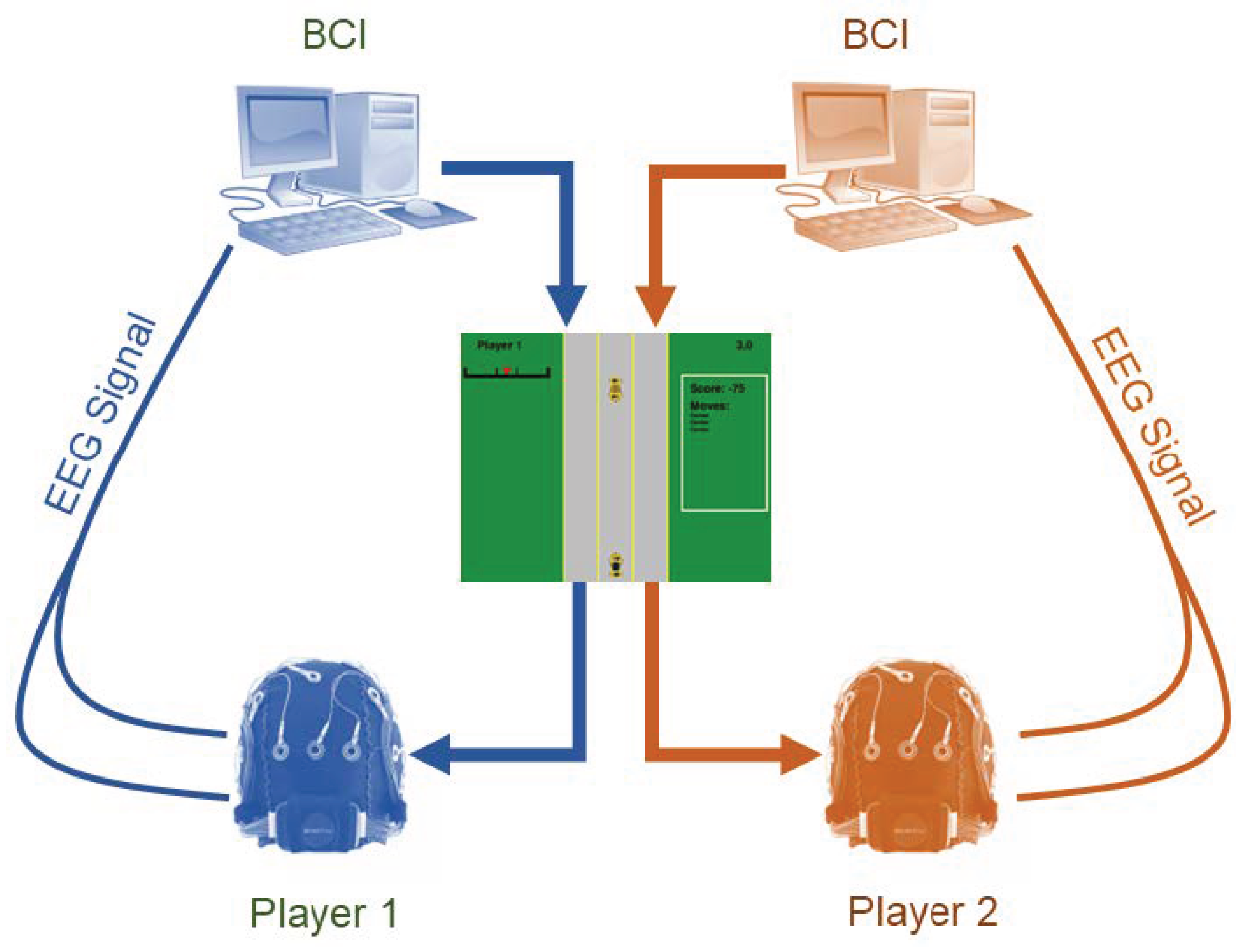
Figure 2.
Dynamical structure of the EEG-driven game interaction. The game visualization produces a stimulus observed by both players. This induces cognitive responses (latent) and EEG signals (observable). Each player’s BCI converts into an action , which jointly determines the next stimulus .
Figure 2.
Dynamical structure of the EEG-driven game interaction. The game visualization produces a stimulus observed by both players. This induces cognitive responses (latent) and EEG signals (observable). Each player’s BCI converts into an action , which jointly determines the next stimulus .
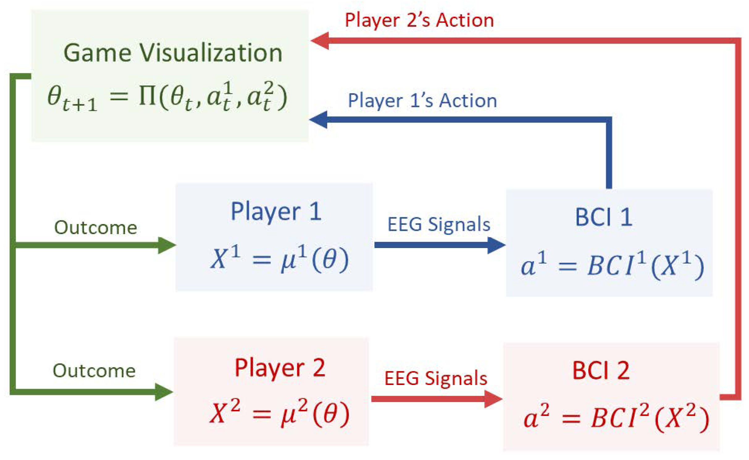
Figure 3.
Mapping from latent cognitive dynamics to observable EEG signals, DMD-based neural embeddings, and BCI-driven actions. The public stimulus influences all stages of neural processing and induces correlation across players’ neurocognitive states.
Figure 3.
Mapping from latent cognitive dynamics to observable EEG signals, DMD-based neural embeddings, and BCI-driven actions. The public stimulus influences all stages of neural processing and induces correlation across players’ neurocognitive states.
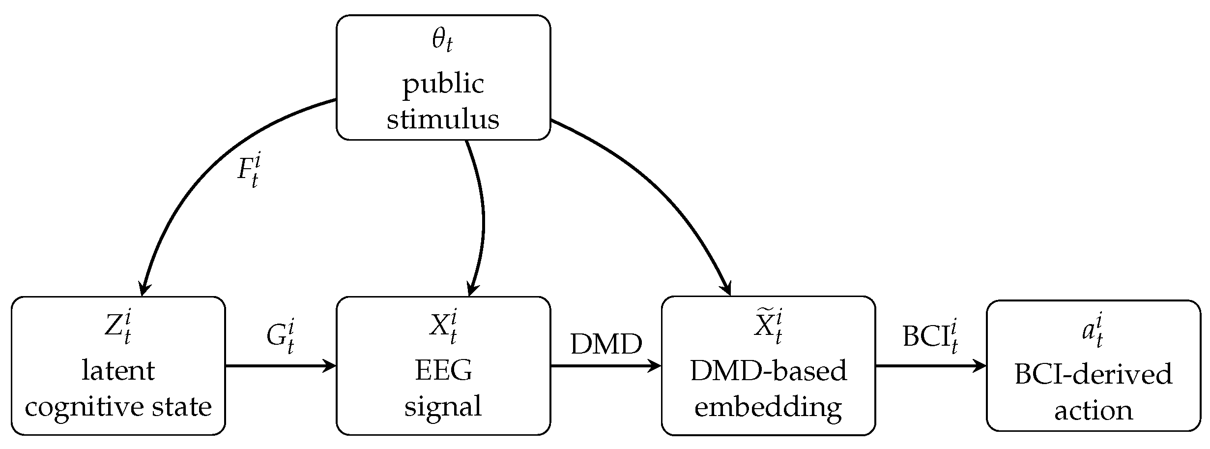
Figure 4.
Directed neural network extracted from thresholded DMD matrices. Nodes are EEG channels for Players 1 and 2; edges represent the strongest inferred dynamical influences. Color intensity reflects outgoing influence magnitude .
Figure 4.
Directed neural network extracted from thresholded DMD matrices. Nodes are EEG channels for Players 1 and 2; edges represent the strongest inferred dynamical influences. Color intensity reflects outgoing influence magnitude .
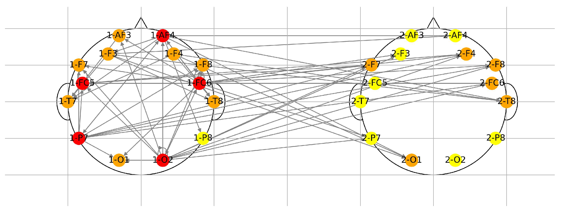
Figure 5.
Average DMD mode energies in the beta band for Player 1. Top: center-action trials. Bottom: swerve-action trials. Color intensity indicates normalized energy contribution . Distributed differences across modes indicate action-dependent neural structure.
Figure 5.
Average DMD mode energies in the beta band for Player 1. Top: center-action trials. Bottom: swerve-action trials. Color intensity indicates normalized energy contribution . Distributed differences across modes indicate action-dependent neural structure.
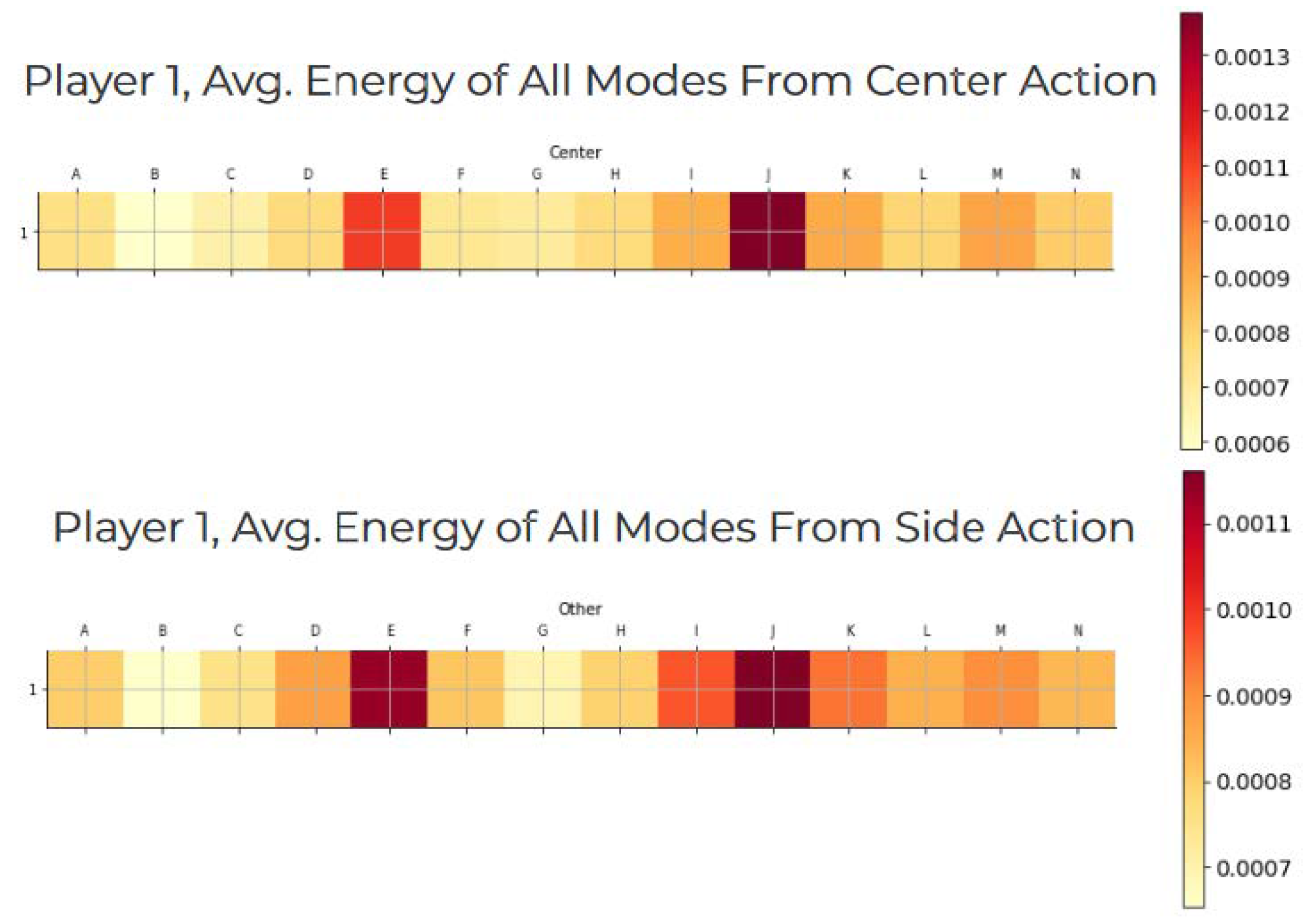

Table 1.
Payoff matrix for the refined three-action chicken game. Entries denote payoffs to Players 1 and 2.
Table 1.
Payoff matrix for the refined three-action chicken game. Entries denote payoffs to Players 1 and 2.
| C | L | R | |
|---|---|---|---|
| C | |||
| L | |||
| R |
Disclaimer/Publisher’s Note: The statements, opinions and data contained in all publications are solely those of the individual author(s) and contributor(s) and not of MDPI and/or the editor(s). MDPI and/or the editor(s) disclaim responsibility for any injury to people or property resulting from any ideas, methods, instructions or products referred to in the content. |
© 2025 by the authors. Licensee MDPI, Basel, Switzerland. This article is an open access article distributed under the terms and conditions of the Creative Commons Attribution (CC BY) license (http://creativecommons.org/licenses/by/4.0/).
Copyright: This open access article is published under a Creative Commons CC BY 4.0 license, which permit the free download, distribution, and reuse, provided that the author and preprint are cited in any reuse.


