
Submitted:
24 December 2025
Posted:
25 December 2025
You are already at the latest version
Abstract
We examine whether aggregate “music mood” derived from globally popular songs can help forecast primary equity issuance. We build a Friday-anchored weekly panel that merges SEC EDGAR counts of priced Initial Public Offerings (IPOs) with features from the Spotify Daily Top 200 (audio descriptors such as valence, energy, danceability, tempo, loudness, etc.) and Genius-scraped lyrics. We extract lyric sentiment by tokenizing Genius-scraped lyrics and aggregating lexicon-based affect scores (valence and arousal) into popularity-weighted weekly indices. To address sparsity and regime shifts in issuance, we train a leakage-safe Long Short-Term Memory (LSTM) network on a smoothed target—the forward 4-week sum of IPOs—and obtain next-week forecasts by dividing the predicted sum by 4. On a chronological holdout, a single LSTM with look-back K=8 outperforms strong baselines—reducing MAE by 13.9%, RMSE by 15.9%, and mean Poisson deviance by 27.6% relative to the best baseline in each metric. Furthermore, we adopt SHapley Additive exPlanations (SHAP) to explain our LSTM model, showing that IPO persistence remains the dominant driver, but music and lyrics covariates contribute incremental and robust signal. These results suggest that aggregate music sentiment contains economically meaningful information about near-term IPO activity.
Keywords:
time series forcasting
; neural networks
; fintech
; IPO activity
1. Introduction
The timing and intensity of initial public offerings (IPOs) are famously cyclical, clustering into “hot” and “cold” markets that are only partially explained by fundamentals [1,2,3]. A large literature links IPO waves to capital market conditions, investor sentiment, and information frictions [4]. In parallel, advances in computational social science show that high-frequency, crowd-scale proxies of sentiment—from textual news to search queries and social media—contain predictive information for financial activity [5,6].
This paper asks a simple question: do aggregate mood signals derived from popular music help forecast near-term IPO activity? The intuition is that the music people stream each day reflects contemporaneous affect, attention, and energy at scale; such changes in mood may co-move with risk appetite and issuance windows, much like weather, sports, or social media shocks have been shown to correlate with market outcomes [7,8]. Unlike sporadic textual events, music consumption yields dense, globally consistent time series with rich acoustic (e.g., valence, energy) and lyrics content that can be aggregated into leak-free weekly indices.
Methodologically, we fuse (i) priced IPO count from SEC EDGAR with robust index retrieval, and (ii) daily Top-200 Spotify features and Genius-derived lyrics processed into popularity-weighted mood measures (e.g., means, dispersion, end-of-week shocks, and lyrics–audio dissonance). We then train a leakage-safe sequence model (LSTM) on a smoothed forward 4-week target to forecast next-week IPO counts, comparing against strong persistence and Poisson Generalized Linear Model (GLM) baselines. LSTMs and related recurrent architectures are a natural fit for nonlinear, regime-switching time series in finance [9,10], and our design emphasizes reproducibility and strict temporal alignment.
On a chronological holdout, we evaluate metrics on the common test weeks to ensure fair cross-model comparability. A single LSTM with look-back delivers consistent gains over strong baselines (naïve persistence, MA(4), MA(13), Poisson GLM): relative to the best baseline in each metric, the model reduces MAE by approximately 13.9%, RMSE by 15.9%, and mean Poisson deviance by 27.6%. These improvements indicate that a compact sequence model exploiting recent history plus music sentiment captures temporal structure beyond simple smoothing and parametric count processes.
Deep learning models like LSTMs are usually considered as black box and lack of transparency. To interpret the model and understand the importance of features, we use SHAP [11] analysis. Global attributions from SHAP show that IPO persistence features (recent lags and moving averages) dominate importance, while contemporaneous music and lyrics covariates contribute incremental signal that improves short-horizon calibration. The explainability results suggest that aggregate music sentiment carries economically meaningful information about near-term IPO windows, even after accounting for persistence and seasonality.
Our main contributions are:
- A reproducible, Friday-anchored weekly panel merging EDGAR IPO count with popularity-weighted music mood indices from audio features and lyrics, with leak-free aggregation.
- Feature primitives tailored to issuance timing (within-week dispersion, end-of-week shocks, lyrics–audio dissonance) that complement standard persistence and seasonality.
- Evidence that a lightweight LSTM trained on a smoothed count target outperforms naïve, MA, and Poisson GLM baselines on a common evaluation window.
- SHAP analyses confirm that music/lyrics covariates provide incremental predictive content alongside IPO persistence and make our model transparent.
Our study connects four strands of research: (i) IPO waves and issuance timing [2,3,4]; (ii) sentiment and markets using textual and alternative data [5,6,8]; (iii) deep learning for financial time-series forecasting [9,10]; and (iv) explainable AI for deep models and financial decision-making, where we employ SHAP to attribute predictions [11]. On affect modeling, we build on lexicon-based approaches to valence/arousal estimation [12,13]. To our knowledge, this is among the first studies to combine large-scale music mood (audio and lyrics) with issuance forecasting and to provide model-consistent, SHAP-based evidence that these covariates add incremental predictive content beyond persistence and seasonality.
The structure of the paper is as follows: Section 2 provides a comprehensive related literature to our work; Section 3 describes data collection and preprocessing; Section 4 presents the methodology; Section 5 reports experimental results and SHAP-based explanations; Section 6 concludes and discusses limitations and future work.
2. Related Literature
IPO timing and issuance cycles. IPO activity is well known to cluster into “hot” and “cold” markets that are only partially explained by fundamentals. Classic and modern accounts attribute waves to time–varying adverse selection, information frictions, and learning [2,3,14]. Surveys synthesize evidence on market conditions, risk appetite, and institutional frictions shaping issuance [4]. Microstructure and cross-sectional studies document that issuers time offerings to exploit windows of investor demand and valuation [1,15]. Our forecasting target—near–term IPO counts—directly connects to this literature by quantifying short–horizon variation in issuance intensity.
Investor sentiment and alternative data. A large body of work links sentiment to market outcomes. Media tone, dictionaries tailored to financial text, and search/attention proxies predict returns, flows, and corporate actions [5,6,16]. Crowd–scale social data also carry predictive content [17,18]. Beyond text, mood proxies such as weather and national sports outcomes affect risk taking and prices [7,8]. Baker and Wurgler’s sentiment index links broad risk appetite to issuance dynamics [19]. We extend this strand by proposing aggregate music mood—constructed from globally popular tracks’ audio and lyrics—as a dense, internationally consistent sentiment proxy that complements event–driven textual measures.
Deep learning for financial time series. Recurrent and attention–based architectures capture nonlinear dynamics, regime changes, and mixed short/long memory in financial series. LSTMs improve equity prediction relative to linear benchmarks and tree ensembles [9]; systematic reviews summarize deep architectures for financial forecasting [10]. Hybrid pipelines combining denoising and feature learning with recurrent models further stabilize training on noisy data [20]. Recent sequence models (e.g., Temporal Convolutional Networks and Transformers) offer competitive performance and built–in mechanisms for handling seasonality and covariates [21,22]. Additionally, generative AI methods, such as Large Language Models (LLMs), demonstrate their ability to answer questions about financial time series [23,24]. Our design adopts a leakage–safe LSTM trained on a smoothed count target tailored to sparse, bursty issuance.
Explainable AI (XAI) for deep models and financial decisions. The adoption of complex models in finance raises transparency and accountability concerns. Model–agnostic tools such as LIME and SHAP attribute predictions to features via local surrogates and game–theoretic values [11,25], while surveys and critical perspectives discuss their promises and limits [26,27,28]. On the other hand, differential equations provide an explicit framework for modeling neural network dynamics, which can enhance explainability and improve resistance to adversarial attacks [29,30,31]. In financial contexts, XAI has been applied to credit risk, market risk, and asset allocation to support validation and governance [32,33,34]. We use SHAP to document where our LSTM’s gains arise: global attributions show IPO persistence dominates, whereas contemporaneous music and lyrics covariates provide incremental signal concentrated in recent lags—evidence that music–based sentiment adds economically meaningful information beyond persistence and seasonality.
Affect modeling foundations. Our construction of mood indices builds on lexicon–based emotion resources (valence and arousal) that have been widely used for large–scale affect measurement [12,13], alongside domain–specific financial dictionaries [6]. The audio side connects to music–information–retrieval studies on mood from acoustic features [35,36]. Relative to prior sentiment proxies, music consumption yields dense, globally consistent time series that can be aggregated into leak–free weekly indices for issuance forecasting.
Relative to (i) the IPO–timing literature, we introduce a new, high–frequency mood proxy; relative to (ii) sentiment and alternative–data studies, we show that music–based sentiment contributes incremental predictive power for issuance counts; relative to (iii) deep time–series forecasting, we pair a leakage–safe target with a lightweight LSTM; and relative to (iv) XAI in finance, we provide SHAP–based evidence clarifying that improvements do not stem solely from persistence or calendar effects.
3. Data
3.1. U.S. IPO Activity from EDGAR (2017–2023)
We construct weekly counts of U.S. initial public offerings (IPOs) from the SEC EDGAR system for 2017–2023. Consistent with market practice, we identify priced IPOs via 424B4 (final prospectus), explicitly excluding 424B2 structured notes:
Events are timestamped by EDGAR date_filed. We aggregate to Friday-anchored weeks using a Saturday 00:00 boundary. Let map a calendar date to the corresponding week start (Saturday). For issuer i (identified by CIK), define the IPO event sets in week w:
We then construct distinct-issuer counts per week
which prevents multiple same-week filings by the same issuer from inflating totals.
The time series in Figure 1 displays pronounced clustering of issuance into windows separated by droughts. From 2017 through 2019, weekly IPO activity is relatively moderate. Activity accelerates through 2020 and peaks in 2021 with several exceptionally high weeks, indicating a pronounced “hot market” episode. Thereafter, counts contract sharply in 2022–2023, with lower average levels and reduced volatility, and occasional near-zero weeks. This figure motivates a forecasting model that handles zero inflation and strong serial dependence.
The Figure 2 reports the year–level average of weekly IPO counts from 2017–2023. Activity is relatively muted and stable in 2017–2019 (about 5.3, 7.3, and 6.8 IPOs per week, respectively), followed by a sharp boom in 2020 (13.1) that culminates in an exceptional peak in 2021 (23.8 average IPOs per week). Issuance then cools markedly in 2022 (5.6), with a modest rebound in 2023 (6.1). The pattern highlights a pronounced 2020–2021 IPO wave and a reversion toward pre-boom levels thereafter.
3.2. Music Features (Spotify Top 200)
We use the Spotify Daily Top 200 (Global) dataset as explanatory variables. Our sample spans 2018-01-25 to 2022-01-06. The Top 200 data are obtained from a public, research-oriented distribution on Kaggle1 and include track metadata (title, artist, rank, streams) and per-track audio descriptors.
For each charted track we collect the standard Spotify audio descriptors: danceability, energy, key, loudness, mode, speechiness, acousticness, instrumentalness, liveness, valence, and tempo. These features serve as daily covariates summarizing the prevailing musical mood and acoustic profile of globally popular songs.
We fetch lyrics via the Genius API2 by querying with the song title and first listed artist. Extracted text is lightly normalized by removing prefaces (e.g., content before “Lyrics”), stripping bracketed section headers (e.g., [Chorus]), collapsing whitespace, and trimming ads/embeds, yielding a single cleaned lyric string per track aligned to the Spotify Top 200 entries. We compute continuous valence and arousal via a word-level lexicon with VAD scores [12].
3.3. Feature Engineering and Weekly Aggregation
Popularity weights. Let i index tracks and d index calendar days. When a popularity score is available, we map it to a bounded weight with a small floor to avoid zero–weight entries:
Here and are the global minimum and maximum popularity values computed over the entire sample index (all observed track–day pairs). If popularity is unavailable, we set . All subsequent aggregates use as weights.
Daily standardization and dissonance. To place lyric and audio measures on a comparable within-day scale, we compute day-wise z-scores for each feature (e.g., lyric valence , lyric arousal , audio valence ):
Here and are, respectively, the cross-sectional mean and standard deviation across the Top-200 tracks present on day d; prevents division by zero on degenerate days. We define valence dissonance at the track–day level as
which measures the absolute discrepancy between lyric- and audio-implied valence in standardized units.
Endweek of shocks. Let and be the (popularity-weighted) weekly means, and let and denote the last day’s (Friday) standardized values. We define Friday shocks as
Novelty of the chart. Let be the set of unique track identifiers appearing in week w. The new-entry share is
i.e., the fraction of titles in week w that did not appear in week , which captures turnover and the influx of fresh content.
Persistence (lags and moving averages). We include autoregressive signals of IPO activity:
Seasonality. Let denote the ISO week index of t. We encode annual seasonality with
Merging music features with IPO counts. We align both datasets on a common Friday-anchored weekly key. Let each calendar date map to its week start (Saturday boundary). For forecasting, we shift targets one step ahead (e.g., w-features → predict ) to avoid look-ahead bias.
4. Methodology
4.1. Problem Setup and Notation
Let index weeks (Friday–anchored). Let denote the number of IPOs observed in week t. Our one–step–ahead target is (“IPO_next”). We collect a weekly feature vector comprising music-derived indices, issuance persistence terms, and seasonal controls. To stabilize learning on sparse counts, we train on a smoothed target,
i.e., the 4–week moving sum forward-looking from to . The model predicts ; at inference we invert the transform and divide by 4 to obtain a weekly prediction , then clip to . This preserves leakage safety because is constructed by first shifting to and then applying a forward rolling sum; the last week (with unknown future) is dropped.
4.2. Sequence Construction and Train/Test Split
We adopt a chronological split: the last of weeks form the test set, the remainder the train set. Given a sequence length K, we build overlapping windows
On train (test), windows start at the first index where K prior observations exist in the respective split.
4.3. LSTM Architecture and Optimization
We use a plain LSTM with a single recurrent layer and a linear head:
trained with mean squared error on the smoothed log target:
We optimize with Adam (learning rate ), early stopping on training loss (patience , best weights restored), and learning rate reduction on plateau (factor , patience , floor ). Batch size is set adaptively (up to 32, roughly half the number of training sequences).
5. Experimental Results
5.1. Evaluation Metrics
Primary evaluation is on the weekly scale using the one–step–ahead target :
We also report Poisson deviance on weekly predictions,
with clipped to be nonnegative.
5.2. Baselines
Let t index Friday–anchored weeks and denote the IPO count in week t. The one–step–ahead prediction target is (“IPO_next”). We evaluate all baselines on the same chronological split as the LSTM: the last of weeks form the test set; earlier weeks form the train set. Seasonality controls use the ISO week number encoded via and .
Naïve last-value. A persistence benchmark that predicts the next week by the current week’s count:
This captures the short-run clustering of issuance and is leakage-safe.
Moving-average (MA) baselines. We include two smoothers that average recent weeks to reduce noise:
MA(4) targets monthly seasonality; MA(13) approximates a quarter. Both are computed recursively on the full timeline so that the test segment can use trailing train observations without look-ahead.
Poisson GLM. To provide a strong classical count model, we fit a generalized linear model with Poisson mean and log link using only lagged IPO dynamics and seasonal terms:
Here collects ; parameters are estimated on the training window by maximum likelihood. Predictions are nonnegative by construction.
For each baseline, we report mean absolute error (MAE), root mean squared error (RMSE), and Poisson deviance on over the test weeks in Table 1. All models are evaluated on the same set of common prediction weeks. MAE is mean absolute error; RMSE is root mean squared error; Poisson Dev. is mean Poisson deviance, computed on nonnegative predictions. The LSTM trained on the smoothed 4-week sum achieves the best scores across all metrics: (i) MAE improves by over the best baseline (Naive), (ii) RMSE improves by over the best baseline (MA(4)), and (iii) Poisson deviance improves by over the best baseline (MA(4)). These gains indicate that the sequence model captures temporal structure beyond simple persistence/smoothing and a parametric Poisson GLM with seasonal controls.
The realized series in Figure 3 is shown against Naive, MA(4), MA(13), Poisson GLM, and the LSTM (K=8). The LSTM captures level shifts with less delay and avoids the GLM’s extreme spikes during volatile periods; MA(13) is overly smoothed and lags peaks/troughs, while Naive and MA(4) respond faster but fail to anticipate reversals.
5.3. Ablation on Sequence Length K.
We vary the LSTM look-back window (weeks of history) while keeping the architecture (1-layer LSTM, 16 units, dropout 0.3) and training setup fixed. The model is trained to predict and mapped back to a weekly forecast by dividing the predicted 4-week sum by 4 (clipped at 0). For a fair comparison across K, all metrics (MAE, RMSE, mean Poisson deviance) are computed on the same 43-week test window. Results in Table 2 show that achieves the lowest MAE, while attains nearly identical RMSE and Dev, so we adopt for the main LSTM results.
5.4. SHAP Explanation Experiment (LSTM, )
Our objective in this subsection is to explain the next-week IPO forecaster (LSTM with look-back ) that is trained on the target . At inference we map back via and report weekly . We use the same chronological split as modeling. Features comprise IPO count, IPO persistence (lags , moving averages ), seasonality (week_sin, week_cos), and music sentiment features (audio and lyric sentiment). Our LSTM to explain is a single-layer LSTM (16 units, dropout 0.3) → Dense(1), Adam (lr ), MSE loss on . We adopt KernelExplainer to obtain model-agnostic SHAP values and aggregate them over time by reporting per feature.
Figure 4 shows that IPO persistence dominates the explanation: ipo_count_ma4,
ipo_count_ma12, ipo_count, ipo_count_lag1, and ipo_count_lag2 have the largest contributions. Music/lyrics covariates (e.g., valence_audio_z_vol, lyrics_valence_shock) provide secondary signal, while seasonality is modest.
Dispersion of audio valence (valence_audio_z_vol) summarizes the cross–track spread of perceived positivity in the globally popular songs during week t. Higher dispersion (i.e., a wider distribution of audio valence) indicates a less concentrated mood state in the listening population—consistent with elevated uncertainty, polarization, or mixed risk appetite. The LSTM assigns sizable importance to this dispersion measure, suggesting that how variable collective mood is can be as informative as where the mean mood sits when anticipating near–term issuance intensity.
End–of–week shocks in lyrics valence (lyrics_valence_shock) captures within–week changes in the semantic polarity of lyrics (popularity–weighted), with an end–of–week focus designed to align with our Friday anchor. Large positive (negative) shocks reflect sudden improvements (deteriorations) in the textual affect of widely streamed songs, plausibly tracking rapid shifts in attention and sentiment. The model’s high SHAP attributions on this shock variable indicate that recent, abrupt changes in crowd–level mood contain incremental information about next–week IPO timing beyond smoother persistence and seasonality patterns.
Together, dispersion in audio valence and shocks in lyrical valence map onto two distinct behavioral channels: (i) uncertainty/heterogeneity in prevailing affect (captured by dispersion), and (ii) salient short–run updates in perceived mood (captured by shocks). These signals complement the persistence features: while lags/MAs encode slowly evolving issuance regimes, the music–derived measures provide high–frequency cues about shifts in risk appetite and attention that are not fully captured by historical IPO dynamics.
The heatmap in Figure 5 visualizes time–by–feature attributions for the most recent explained case (columns to , rows are features). Three patterns emerge.
(i) Short-memory concentration. Most attribution mass occurs at and , consistent with short-horizon issuance dynamics. In particular, ipo_count_lag2 and ipo_count_lag8 receive large positive contributions near , while a smaller seasonal component appears far back at for ipo_count. Older timesteps ( to ) contribute little, indicating that the LSTM emphasizes very recent history.
(ii) Incremental music/lyrics signal. Two non-persistence covariates stand out at the end of the window. lyrics_valence_shock loads heavily at , implying that a sharp within-week change in lyrical polarity immediately precedes higher (or lower) predicted issuance. valence_audio_z_vol contributes moderately at , consistent with contemporaneous affect in listening behavior complementing persistence cues.
(iii) Transient composition effects. We observe a localized spike at in new_entry_share (share of newly entering tracks in the Top 200). These mid-window attributions suggest occasional composition shocks in the popular-music basket—e.g., a burst of new releases or faster songs—that the model treats as informative but transient signals relative to last-week dynamics.
The heatmap supports the global-bar findings: persistence features dominate, but recent music/lyrics variables provide incremental information right before the forecasted week. The temporal localization of attributions to and aligns with a short effective memory for IPO intensity, while sparse mid-lag spikes reflect episodic, high-salience updates in the music-based covariates.
6. Conclusion
This paper introduces a reproducible pipeline that (i) builds issuance targets from SEC EDGAR with priced–offering screens and robust index fallbacks, (ii) derives daily, popularity–weighted music features from the Spotify Daily Top 200 and cleaned Genius lyrics, and (iii) aggregates them into leakage–safe, Friday–anchored weekly predictors (means, end–of–week shocks, dispersion, lyrics–audio dissonance, and related covariates). We train a leakage–safe LSTM on a smoothed forward 4-week target and obtain next-week forecasts by dividing the predicted sum by four.
On a chronological holdout, evaluating models on the common test window ( weeks), a single LSTM with look-back outperforms strong baselines—naïve persistence, MA(4), MA(13), and a Poisson GLM with seasonality—reducing error by 13.9% in MAE, 15.9% in RMSE, and 27.6% in mean Poisson deviance relative to the best baseline for each metric. These gains indicate that a lightweight sequence model, trained on a stabilized count target, captures temporal structure beyond simple smoothing and parametric count processes.
To interpret the model, we apply SHAP to the LSTM. Global attributions show that IPO persistence features (recent lags and moving averages) dominate importance, while contemporaneous music/lyrics covariates contribute incremental and robust signal; per-example heatmaps reveal that contributions concentrate on recent timesteps, consistent with short-horizon issuance dynamics. Taken together, these findings suggest that aggregate music sentiment carries economically meaningful information for near-term IPO activity, complementing persistence and calendar seasonality.
Our results motivate incorporating high-frequency cultural signals into issuance forecasting and monitoring (e.g., window-timing dashboards). Future work could (i) extend to SEOs and cross-market issuance, (ii) test alternative architectures (temporal CNNs/Transformers) and multitask targets (e.g., intensity and zero-inflation), (iii) refine affect modeling beyond lexicons (contextual embeddings for lyrics; non-linear audio sentiment), and (iv) study causality and stability under regime shifts via rolling/bootstrapped evaluations and policy-relevant stress tests.
6.1. Theoretical contribution
We introduce a novel channel for market prediction by constructing large-scale music-based mood indices from audio features and lyrics. This extends the expanding literature on alternative sentiment sources—including news tone [5], financial text dictionaries [6], search-based attention [16,37], social-media mood [17,38] and lyrics only metrics [39]— by demonstrating that cultural-mood signals from both sonic and lyrical features contain predictive information relevant for capital markets.
Our study contributes to the literature on IPO timing by providing new evidence on the role of investor sentiment. First, we construct a novel music-based sentiment index that captures broad investor mood while remaining plausibly orthogonal to IPO-specific institutional features, such as regulatory calendars, reporting cycles, and underwriting capacity. Second, exploiting within-wave variation in IPO issuance, we show robust evidence that sentiment helps explain fluctuations in IPO volume beyond fundamentals [3] and mechanical seasonality. Using explainable-AI methods, we further decompose predictive contributions and demonstrate that music-based sentiment provides economically meaningful incremental information relative to persistence and calendar-based predictors traditionally used to model IPO activity.
6.2. Methodological Contribution
First, we develop a reproducible, leakage-safe forecasting pipeline anchored on a Friday-based weekly dataset with forward-looking smoothing targets, chronological splits, and temporal alignment. These design principles address the field’s emphasis on rigorous, time-ordered AI modeling, where data leakage represents a challenge to the validity of sequential prediction systems [10]. Second, we demonstrate that a compact LSTM model [9,40] significantly outperforms naïve persistence, moving-average baselines, and Poisson generalized linear models with seasonality in forecasting next-week IPO counts. This finding contributes to the growing evidence that deep architectures effectively capture the nonlinear, regime-switching dynamics characteristic of financial time series [10,22]. Third, we employ SHAP [11] to interpret our LSTM model, addressing the critical need for transparency in financial AI systems. This approach aligns with increasing regulatory and practitioner emphasis on explainability and auditability in financial machine learning [26,28,32].
6.3. Implications for Practitioners
Our findings show that cultural-mood indicators can enhance algorithmic issuance calendars, syndicate-desk dashboards, investor-sentiment monitors, and real-time risk assessments. By integrating music-derived sentiment signals, our study offers several operational pathways. Issuance desks and underwriters can utilize music-based mood indicators as early-warning signals for favorable or unfavorable issuance windows. Positive mood shocks—such as sudden increases in lyrical valence—may signal elevated investor risk appetite and optimal timing for new filings [1,19]. This capability enables syndicate desks to refine their go-to-market timing strategies based on real-time cultural sentiment. FinTech market-intelligence providers can incorporate mood indices into analytics dashboards as complementary sentiment measures alongside traditional indicators such as news tone, search volume, and social-media sentiment [5,18]. The distinctive information content of music-based signals offers a unique value proposition within sentiment-monitoring markets.
Author Contributions
The conceptualization, methodology, validation, formal analysis, investigation, and writing of the paper were completed by all authors equally. All authors have read and agreed to the published version of the manuscript.
Data Availability Statement
The data presented in this study are available on request from the corresponding author due to their ongoing use in further analyses related to future research.
Conflicts of Interest
The authors declare no conflicts of interest.
| 1 | |
| 2 |
References
- Lowry, M. Why does IPO volume fluctuate so much? Journal of Financial economics 2003, 67, 3–40. [Google Scholar] [CrossRef]
- Lowry, M.; Schwert, G.W. IPO market cycles: Bubbles or sequential learning? The Journal of Finance 2002, 57, 1171–1200. [Google Scholar] [CrossRef]
- Pástor, L.; Veronesi, P. Rational IPO waves. The Journal of Finance 2005, 60, 1713–1757. [Google Scholar] [CrossRef]
- Ritter, J.R.; Welch, I. A review of IPO activity, pricing, and allocations. The journal of Finance 2002, 57, 1795–1828. [Google Scholar] [CrossRef]
- Tetlock, P.C. Giving content to investor sentiment: The role of media in the stock market. The Journal of finance 2007, 62, 1139–1168. [Google Scholar] [CrossRef]
- Loughran, T.; McDonald, B. When is a liability not a liability? Textual analysis, dictionaries, and 10-Ks. The Journal of finance 2011, 66, 35–65. [Google Scholar] [CrossRef]
- Hirshleifer, D.; Shumway, T. Good day sunshine: Stock returns and the weather. The journal of Finance 2003, 58, 1009–1032. [Google Scholar] [CrossRef]
- Edmans, A.; Garcia, D.; Norli, Ø. Sports sentiment and stock returns. The Journal of finance 2007, 62, 1967–1998. [Google Scholar] [CrossRef]
- Fischer, T.; Krauss, C. Deep learning with long short-term memory networks for financial market predictions. European journal of operational research 2018, 270, 654–669. [Google Scholar] [CrossRef]
- Sezer, O.B.; Gudelek, M.U.; Ozbayoglu, A.M. Financial time series forecasting with deep learning: A systematic literature review: 2005–2019. Applied soft computing 2020, 90, 106181. [Google Scholar] [CrossRef]
- Lundberg, S.M.; Lee, S.I. A unified approach to interpreting model predictions. Advances in neural information processing systems 2017, 30. [Google Scholar]
- Mohammad, S. Obtaining reliable human ratings of valence, arousal, and dominance for 20,000 English words. Proceedings of the Proceedings of the 56th annual meeting of the association for computational linguistics (volume 1: Long papers) 2018, 174–184. [Google Scholar]
- Demszky, D.; Movshovitz-Attias, D.; Ko, J.; Cowen, A.; Nemade, G.; Ravi, S. GoEmotions: A dataset of fine-grained emotions. arXiv 2020, arXiv:2005.00547. [Google Scholar]
- Ibbotson, R.G.; Jaffe, J.F. Hot Issue Markets. The Journal of Finance 1975, 30, 1027–1042. [Google Scholar] [PubMed]
- Helwege, J.; Liang, N. Initial Public Offerings in Hot and Cold Markets. Journal of Financial and Quantitative Analysis 2004, 39, 541–569. [Google Scholar] [CrossRef]
- Da, Z.; Engelberg, J.; Gao, P. In Search of Attention. The Journal of Finance 2011, 66, 1461–1499. [Google Scholar] [CrossRef]
- Bollen, J.; Mao, H.; Zeng, X. Twitter Mood Predicts the Stock Market. Journal of Computational Science 2011, 2, 1–8. [Google Scholar] [CrossRef]
- García, D. Sentiment During Recessions. The Journal of Finance 2013, 68, 1267–1300. [Google Scholar] [CrossRef]
- Baker, M.; Wurgler, J. Investor Sentiment and the Cross-Section of Stock Returns. The Journal of Finance 2006, 61, 1645–1680. [Google Scholar] [CrossRef]
- Bao, W.; Yue, J.; Rao, Y. A Deep Learning Framework for Financial Time Series Using Stacked Autoencoders and Long-Short Term Memory. PLOS ONE 2017, 12, e0180944. [Google Scholar] [CrossRef]
- Borovykh, A.; Bohte, S.; Oosterlee, C.W. Conditional Time Series Forecasting with Convolutional Neural Networks. arXiv 2017, arXiv:1703.04691. [Google Scholar]
- Lim, B.; Arık, S.Ö.; Loeff, N.; Pfister, T. Temporal Fusion Transformers for Interpretable Multi-Horizon Time Series Forecasting. International Journal of Forecasting 2021, 37, 1748–1764. [Google Scholar] [CrossRef]
- Ding, Q.; Ding, D.; Wang, Y.; Guan, C.; Ding, B. Unraveling the landscape of large language models: a systematic review and future perspectives. Journal of Electronic Business & Digital Economics 2023, 3, 3–19. [Google Scholar] [CrossRef]
- Lee, D.K.C.; Guan, C.; Yu, Y.; Ding, Q. A comprehensive review of generative AI in finance. FinTech 2024, 3, 460–478. [Google Scholar] [CrossRef]
- Ribeiro, M.T.; Singh, S.; Guestrin, C. Why Should I Trust You?": Explaining the Predictions of Any Classifier. In Proceedings of the Proceedings of the 22nd ACM SIGKDD International Conference on Knowledge Discovery and Data Mining (KDD), 2016; pp. 1135–1144. [Google Scholar]
- Arrieta, A.B.; Díaz-Rodríguez, N.; Del Ser, J.; Bennetot, A.; Tabik, S.; Barbado, A.; García, S.; Gil-López, S.; Molina, D.; Benjamins, R.; et al. Explainable Artificial Intelligence (XAI): Concepts, taxonomies, opportunities and challenges toward responsible AI. Information fusion 2020, 58, 82–115. [Google Scholar] [CrossRef]
- Molnar, C. Interpretable machine learning; Lulu. com, 2020. [Google Scholar]
- Rudin, C. Stop Explaining Black Box Machine Learning Models for High Stakes Decisions and Use Interpretable Models Instead. Nature Machine Intelligence 2019, 1, 206–215. [Google Scholar] [CrossRef]
- Kang, Q.; Song, Y.; Ding, Q.; Tay, W.P. Stable neural ode with lyapunov-stable equilibrium points for defending against adversarial attacks. Advances in Neural Information Processing Systems 2021, 34, 14925–14937. [Google Scholar]
- Kang, Q.; Zhao, K.; Ding, Q.; Ji, F.; Li, X.; Liang, W.; Song, Y.; Tay, W.P. Unleashing the potential of fractional calculus in graph neural networks with FROND. arXiv 2024. arXiv:2404.17099. [CrossRef]
- Zhao, K.; Li, X.; Kang, Q.; Ji, F.; Ding, Q.; Zhao, Y.; Liang, W.; Tay, W.P. Distributed-order fractional graph operating network. Advances in Neural Information Processing Systems 2024, 37, 103442–103475. [Google Scholar]
- Bussmann, N.; Giudici, P.; Marinelli, D.; Papenbrock, J. Explainable Machine Learning in Credit Risk Management. Computational Economics 2021, 57, 203–216. [Google Scholar] [CrossRef]
- Wang, Y.; Ding, Q.; Wang, K.; Liu, Y.; Wu, X.; Wang, J.; Liu, Y.; Miao, C. The skyline of counterfactual explanations for machine learning decision models. In Proceedings of the Proceedings of the 30th ACM International Conference on Information & Knowledge Management, 2021; pp. 2030–2039. [Google Scholar]
- Beckmann, L.; Broszeit, S.; Stieber, S. Understanding the Determinants of Bond Excess Returns Using Explainable Artificial Intelligence. Journal of Business Economics 2023, 93, 1817–1849. [Google Scholar] [CrossRef]
- Hu, X.; Downie, J.S. When Lyrics Outperform Audio for Music Mood Classification: A Feature Analysis. In Proceedings of the Proceedings of the 11th International Society for Music Information Retrieval Conference (ISMIR), 2010; pp. 619–624. [Google Scholar]
- Laurier, C. Automatic Classification of Musical Mood by Content-Based Analysis. PhD thesis, Universitat Pompeu Fabra, 2009. [Google Scholar]
- Mou, J.; Liu, W.; Guan, C.; Westland, J.C.; Kim, J. Predicting the cryptocurrency market using social media metrics and search trends during COVID-19. Electronic Commerce Research 2024, 24, 1307–1333. [Google Scholar] [CrossRef]
- Guan, C.; Liu, W.; Cheng, J.Y.C. Using social media to predict the stock market crash and rebound amid the pandemic: the digital ‘haves’ and ‘have-mores’. Annals of Data Science 2022, 9, 5–31. [Google Scholar] [CrossRef] [PubMed]
- Guan, C.; Yu, Y.; Ren, J.; Ding, D. From Chart to Chart: Analyzing Lyric Content in Music Streaming Charts for Predicting Stock Prices Using LSTM. In Machine Learning and Modeling Techniques in Financial Data Science; IGI Global Scientific Publishing, 2025; pp. 295–320. [Google Scholar]
- Hochreiter, S.; Schmidhuber, J. Long short-term memory. Neural computation 1997, 9, 1735–1780. [Google Scholar] [CrossRef]
Figure 1.
Weekly U.S. IPO counts, 2017–2023 (Friday-anchored weeks). The series exhibits zero inflation and clustered issuance windows.
Figure 1.
Weekly U.S. IPO counts, 2017–2023 (Friday-anchored weeks). The series exhibits zero inflation and clustered issuance windows.
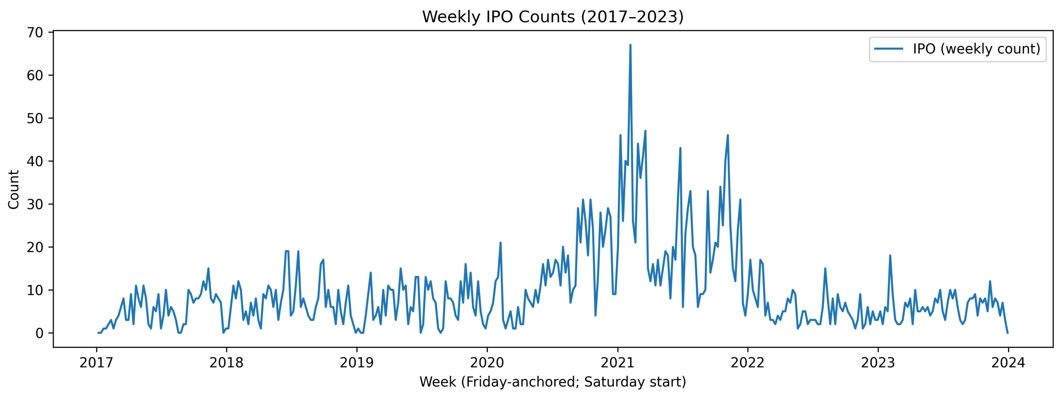
Figure 2.
Average weekly U.S. IPO counts by year (2017–2023). Numbers above bars indicate the annual mean of weekly distinct-issuer IPO counts aggregated from EDGAR.
Figure 2.
Average weekly U.S. IPO counts by year (2017–2023). Numbers above bars indicate the annual mean of weekly distinct-issuer IPO counts aggregated from EDGAR.
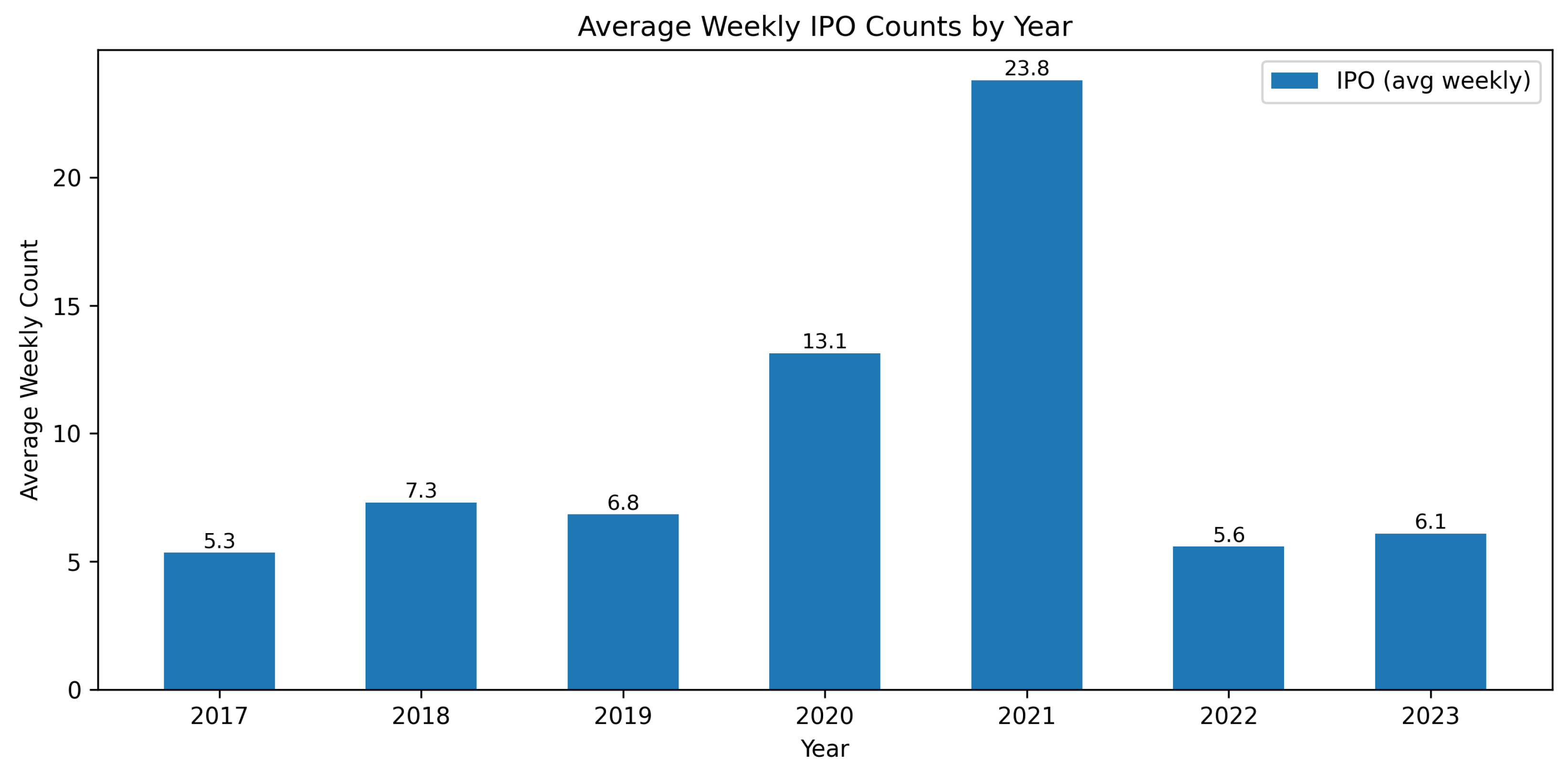
Figure 3.
Next–week IPO forecasts on the common test weeks.
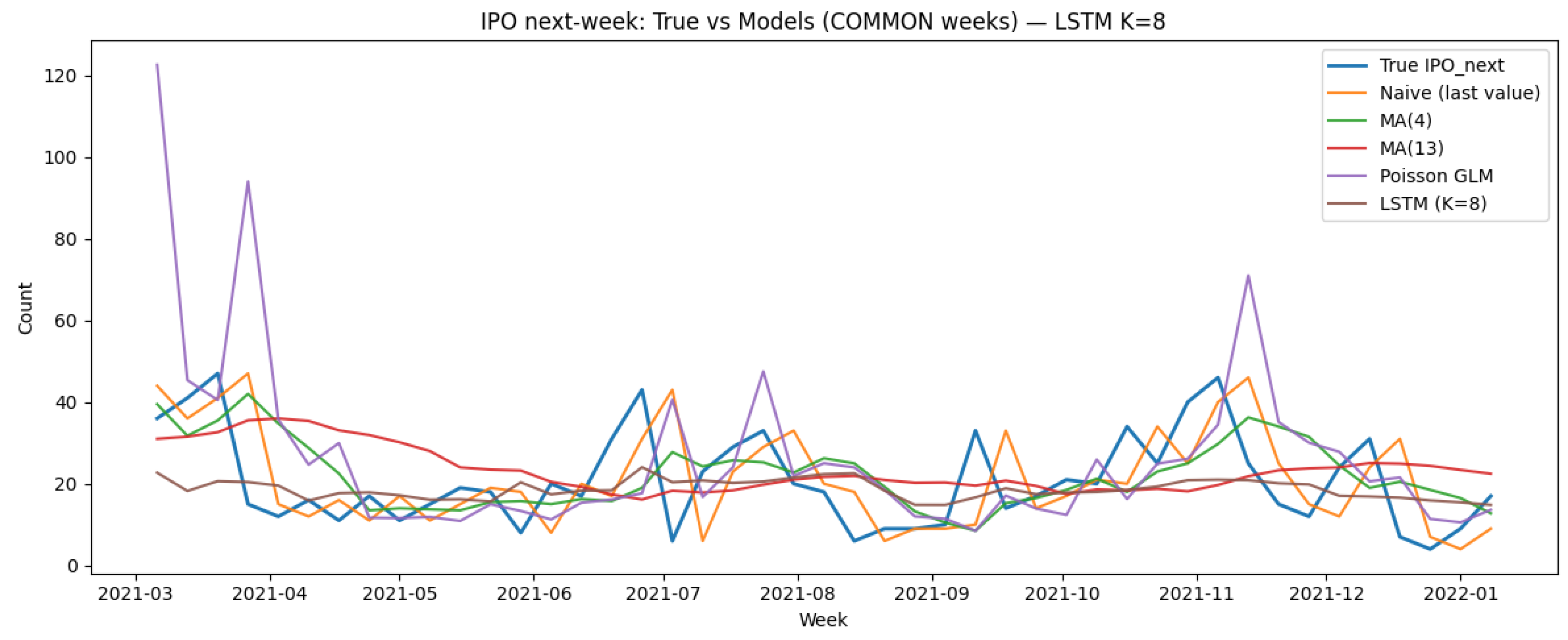
Figure 4.
Global SHAP (KernelExplainer) for the LSTM with , aggregated over time.
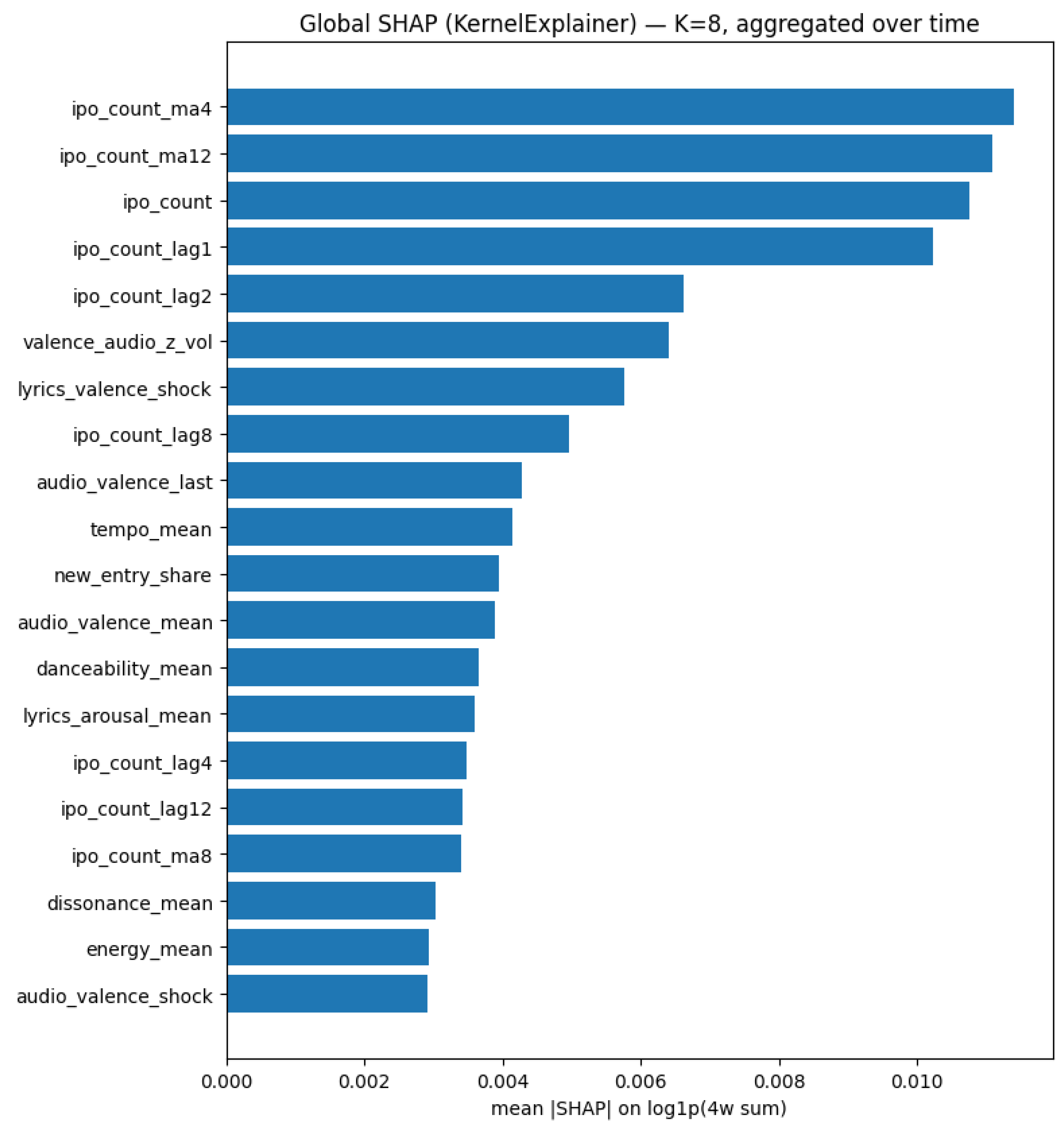
Figure 5.
Per-example SHAP heatmap (last test week explained) for .
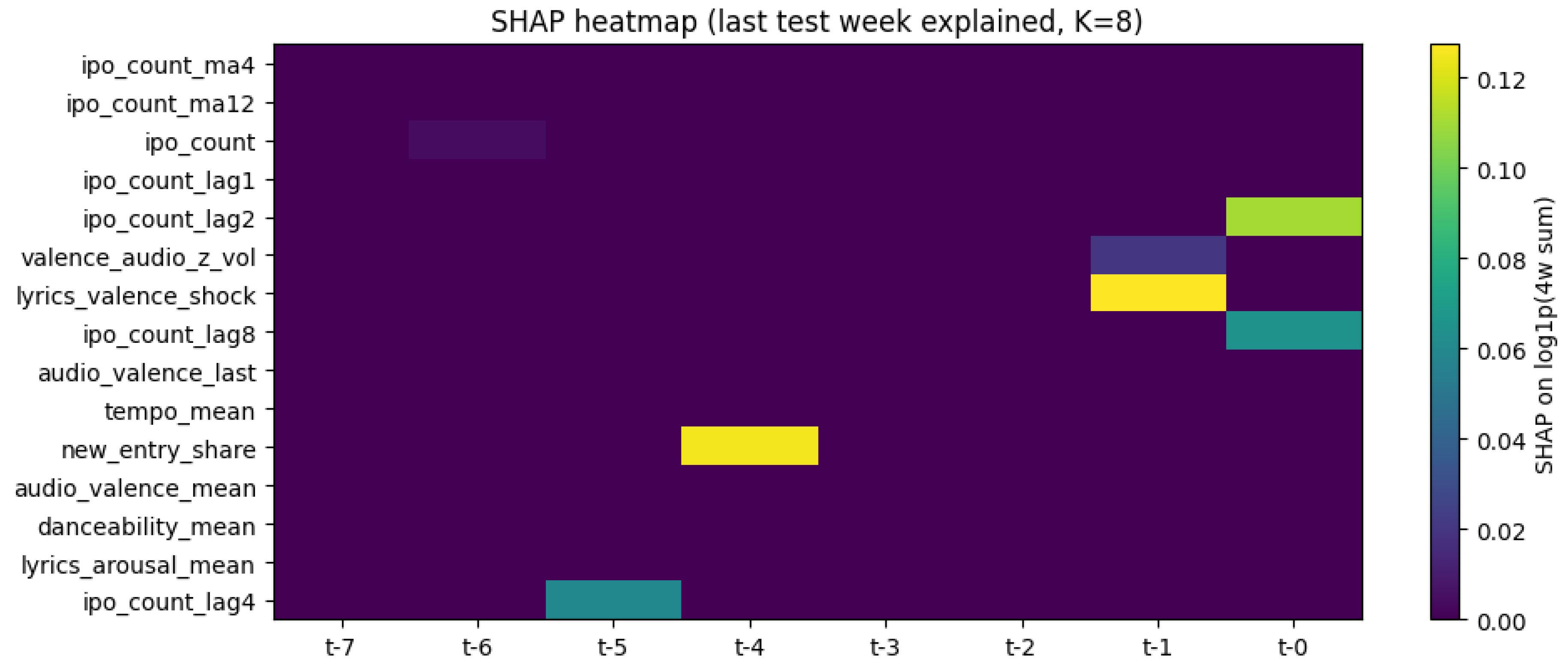

Table 1.
Performance on the common test weeks (intersection across all models; ). Lower is better.
| Model | N | MAE | RMSE | Poisson Dev. |
|---|---|---|---|---|
| LSTM (K=8) | 43 | 8.091 | 10.393 | 5.154 |
| Naive (last value) | 43 | 9.395 | 12.497 | 7.167 |
| MA(4) | 43 | 9.634 | 12.361 | 7.116 |
| MA(13) | 43 | 11.549 | 13.690 | 8.520 |
| Poisson GLM | 43 | 12.277 | 18.638 | 10.421 |
Table 2.
Ablation over sequence length K for next-week IPO prediction. Metrics are computed on the common 43 test weeks (lower is better).
Table 2.
Ablation over sequence length K for next-week IPO prediction. Metrics are computed on the common 43 test weeks (lower is better).
| K | n | MAE | RMSE | Poisson Dev. |
|---|---|---|---|---|
| 2 | 43 | 9.456 | 11.295 | 6.130 |
| 4 | 43 | 8.106 | 10.488 | 5.255 |
| 6 | 43 | 8.208 | 10.380 | 5.148 |
| 8 | 43 | 8.091 | 10.393 | 5.154 |
| 10 | 43 | 8.115 | 10.409 | 5.212 |
Disclaimer/Publisher’s Note: The statements, opinions and data contained in all publications are solely those of the individual author(s) and contributor(s) and not of MDPI and/or the editor(s). MDPI and/or the editor(s) disclaim responsibility for any injury to people or property resulting from any ideas, methods, instructions or products referred to in the content. |
© 2025 by the authors. Licensee MDPI, Basel, Switzerland. This article is an open access article distributed under the terms and conditions of the Creative Commons Attribution (CC BY) license (http://creativecommons.org/licenses/by/4.0/).
Copyright: This open access article is published under a Creative Commons CC BY 4.0 license, which permit the free download, distribution, and reuse, provided that the author and preprint are cited in any reuse.


