Submitted:
23 December 2025
Posted:
24 December 2025
You are already at the latest version
Abstract
This paper proposes an applied framework for cyberattack and anomaly detection in resource-constrained embedded/IoT environments by combining signal-processing feature construction with supervised and unsupervised AI (Artificial Intelligence) models. The workflow covers dataset preparation and normalization, correlation-driven feature analysis, and compact representations via PCA (Principal Component Analysis), followed by classification and anomaly scoring. In addition to the original UNSW-NB15 (University of New South Wales—Network-Based Dataset 2015) traffic features, Fourier-domain descriptors, wavelet-domain descriptors, and Kalman-based smoothing/innovation features are considered to improve robustness under variability and measurement noise. Detection performance is assessed using classical and ensemble learning methods (SVM (Support Vector Machines), RF (Random Forest), XGBoost (Extreme Gradient Boosting), LightGBM (Light Gradient Boosting Machine)), unsupervised baselines (K-Means and DBSCAN (Density-Based Spatial Clustering of Applications with Noise)), and DL (Deep-Learning) anomaly detectors based on Autoencoder reconstruction and GAN (Generative Adversarial Network)-based scoring. Experimental results on UNSW-NB15 indicate that ensemble-based models provide the strongest overall detection performance, while the signal-processing augmentation and PCA-based compactness support efficient deployment in embedded contexts. The findings confirm that integrating lightweight signal processing with AI-driven models enables effective and adaptable identification of malicious network traffic supporting deployment-oriented embedded cybersecurity and motivating future real-time validation on edge hardware.
Keywords:
1. Introduction
2. Literature Review
3. Methodologies
3.1. Collecting Data in Embedded Systems
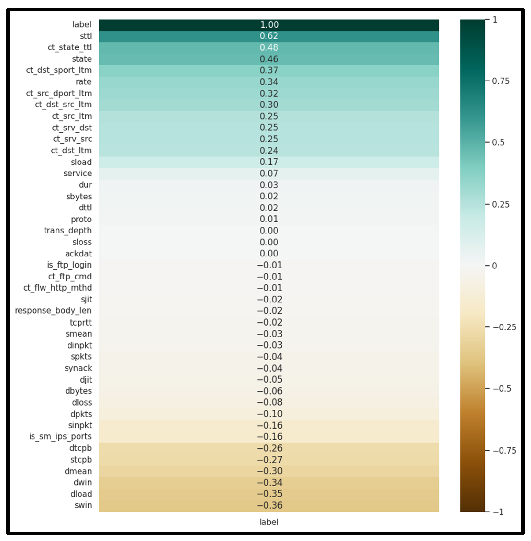
3.2. Analyzing Security Data in Embedded Systems
3.3. Signal Preprocessing Pipeline and Time-Series Construction
3.4. Signal Processing Techniques Used to Detect Anomalies
3.5. AI Models for Cyberattack and Anomaly Detection
4. Implementation and Results
4.1. Embedded Deployment
4.2. Dataset Description and Benchmark Protocol
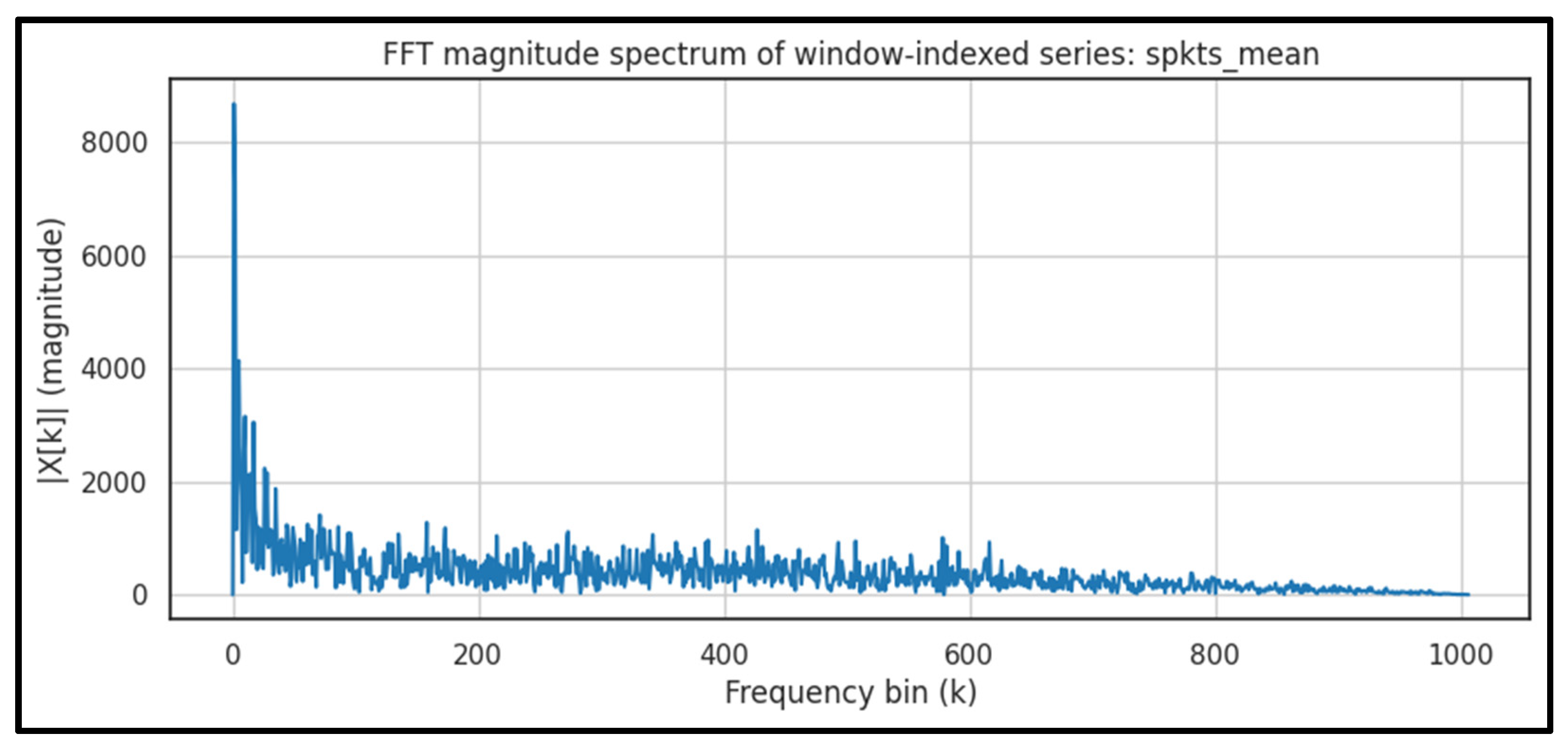
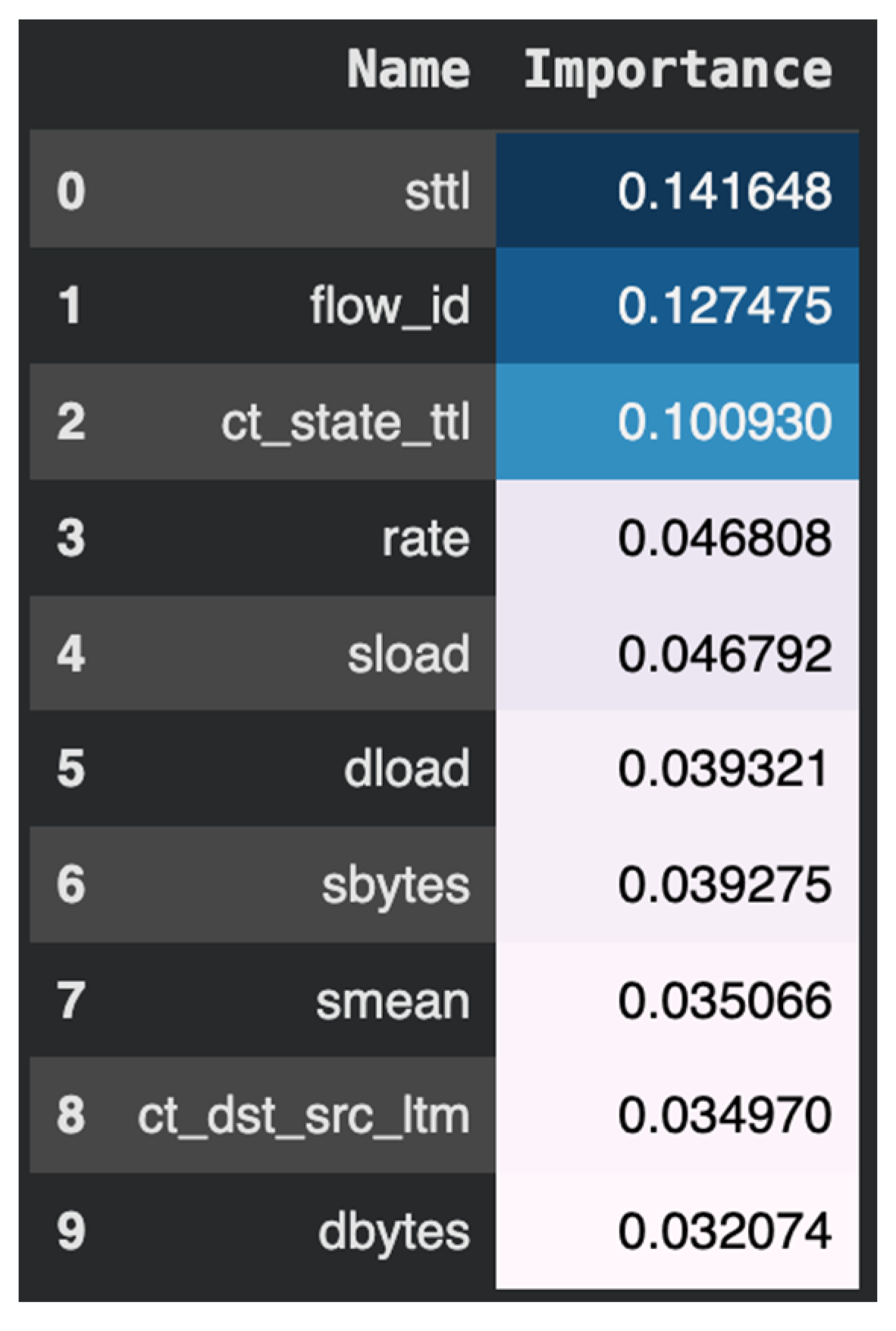
4.3. FFT-Based Feature Representation and Detector Suite
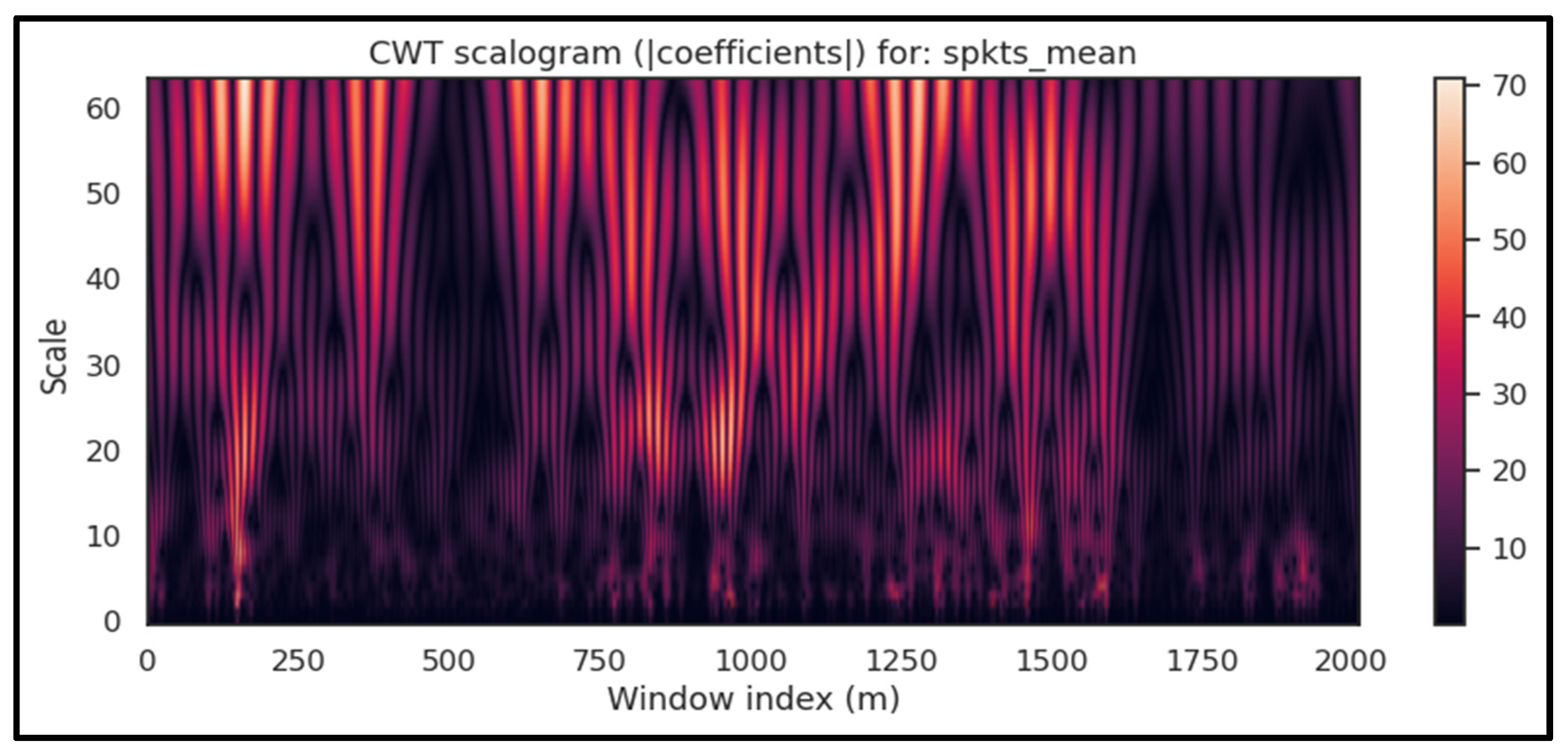
4.4. Wavelet-Based Feature Representation and Detector Suite
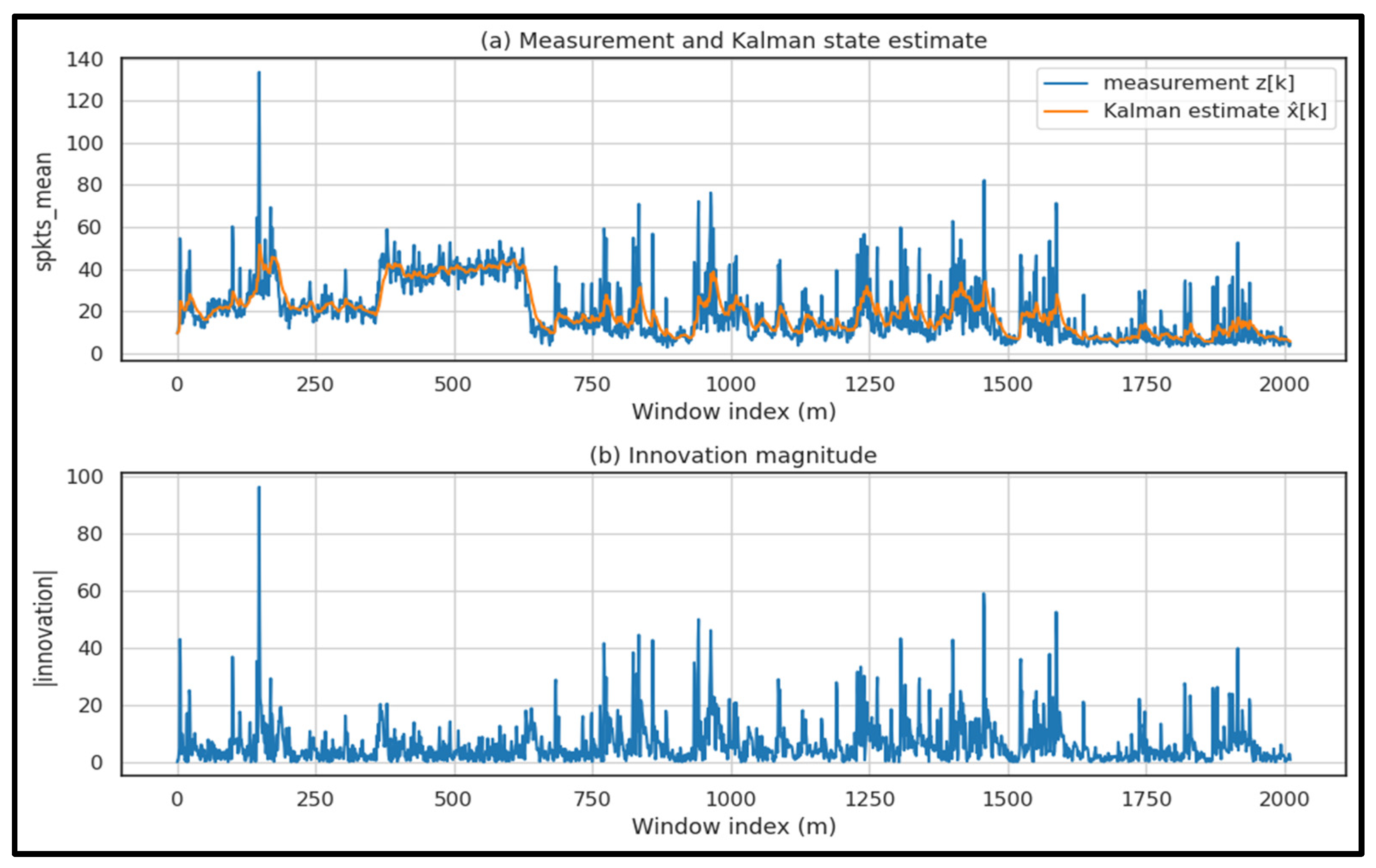
4.5. Kalman-Based Feature Representation and Detector Suite
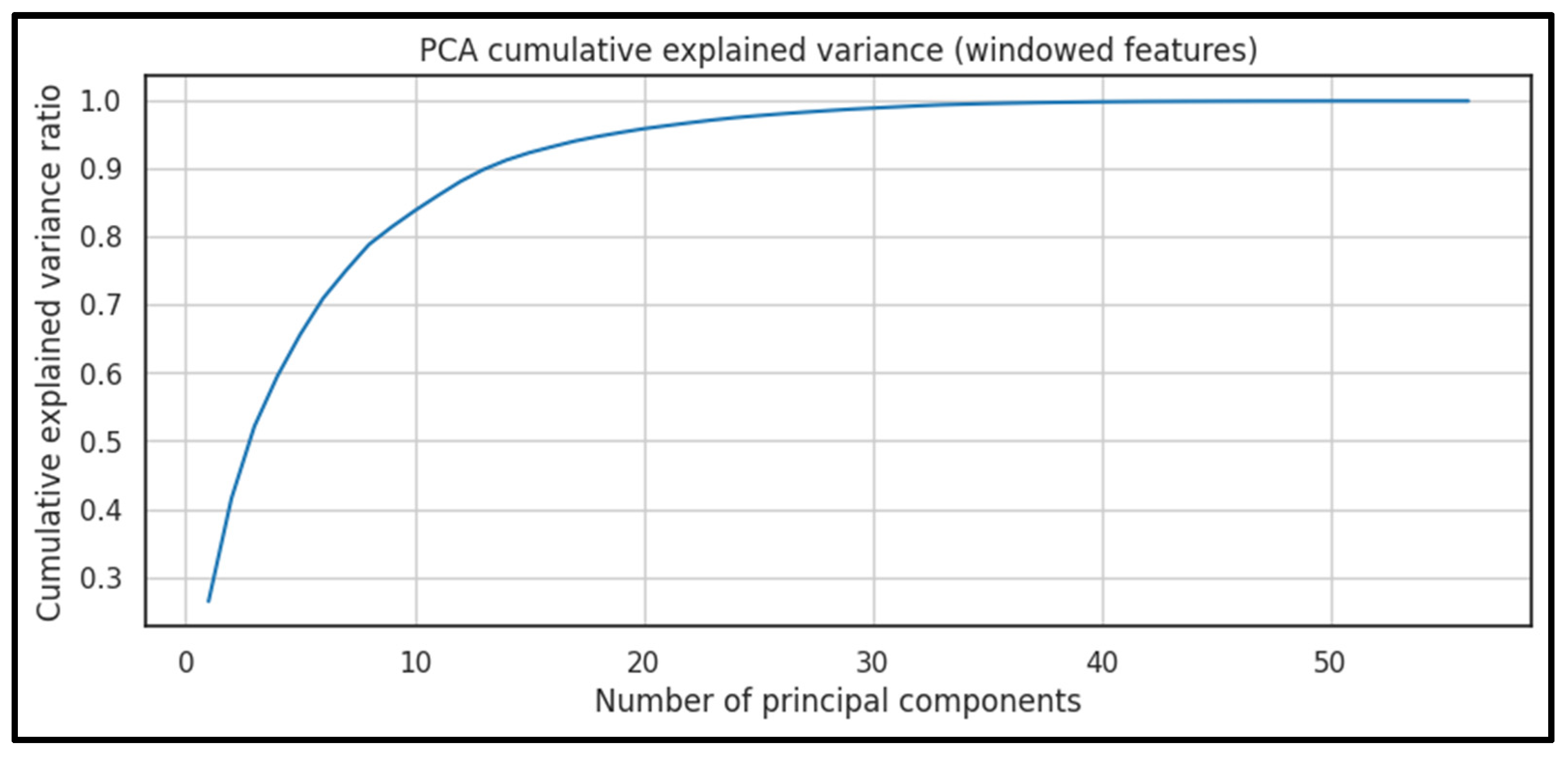
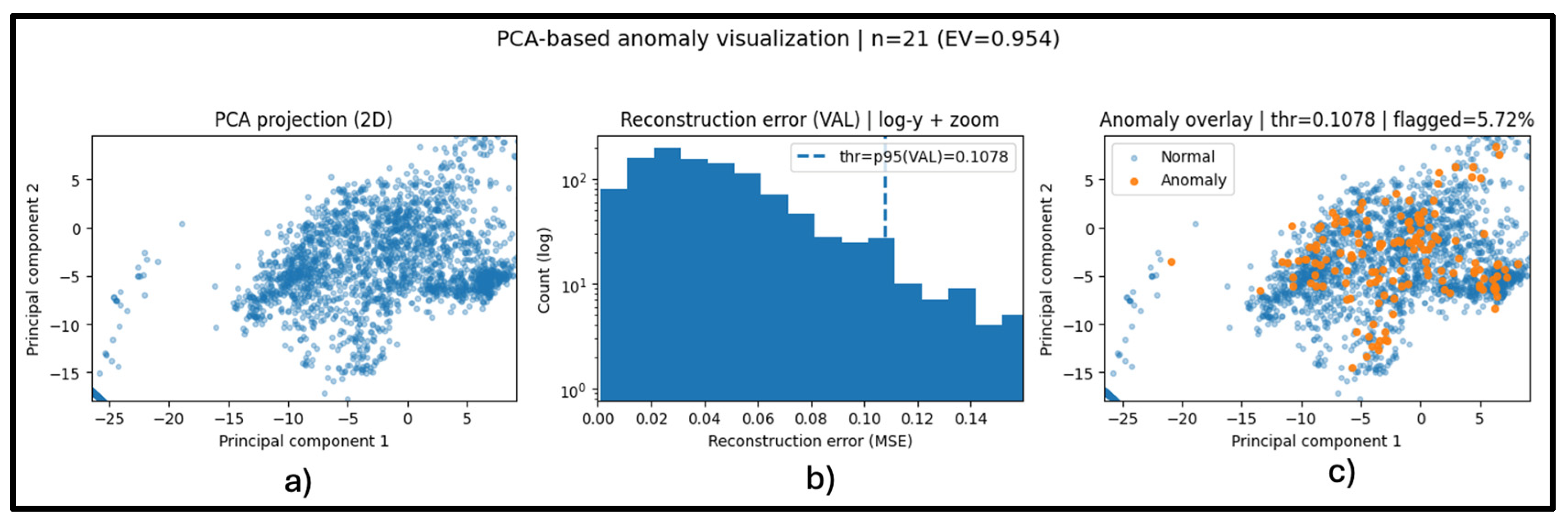
4.6. PCA-Based Feature Representation and Anomaly Visualization
4.7. Embedded Deployment Framework
| Algorithm 1. End-to-End Methodology for Embedded Cyber-Attack Detection |
| Input: |
| - UNSW-NB15 train set Dtrain and test set Dtest (official split) |
| - Window length W, hop H |
| - Descriptor set C (numeric flow attributes) |
| - FFT descriptor subset Cfft ⊂ C |
| - FFT length L, frequency bands B |
| - Final classifier MF (Random Forest, θRF) |
| - Noise levels Σ and random seeds S |
| - Bootstrap resamples R |
| Output: |
| - Trained model MF and final framework metrics |
| - Test metrics (Acc, Prec, Rec, F1, AUC) |
| - Bootstrap 95% CI and robustness (ΔAUC, ΔRec) |
| - Deployment profiling metrics (latency, memory, footprint) |
| 1: Load Dtrain and Dtest using the official UNSW-NB15 predefined split. |
| 2: Select numeric base attributes C from the intersection of train/test columns. |
| 3: For each dataset D ∈ {Dtrain, Dtest}: |
| 4: Segment D into overlapping windows using (W, H). |
| 5: For each window, compute mean/std/min/max for each attribute in C→T(D). |
| 6: Assign window label ywin = 1 if any sample in window is malicious; else 0. |
| 7: For each dataset D ∈ {Dtrain, Dtest}: |
| 8: For each descriptor d ∈ Cfft: |
| 9: Apply sliding rFFT over length L and extract spectral features over bands B. |
| 10: Concatenate features across descriptors → X(D); drop first (L − 1) steps. |
| 11: Split X(Dtrain) into fit/validation (80/20); keep X(Dtest) held out. |
| 12: Train MF on the fit subset using cost-sensitive learning (balanced class weighting). |
| 13: Select the operating threshold and any hyperparameters on validation only. |
| 14: Evaluate MF on held-out test: report Acc/Prec/Rec/F1/AUC and macro/per-class metrics. |
| 15: Bootstrap test instances (R resamples) to estimate 95% CI for AUC (and Rec). |
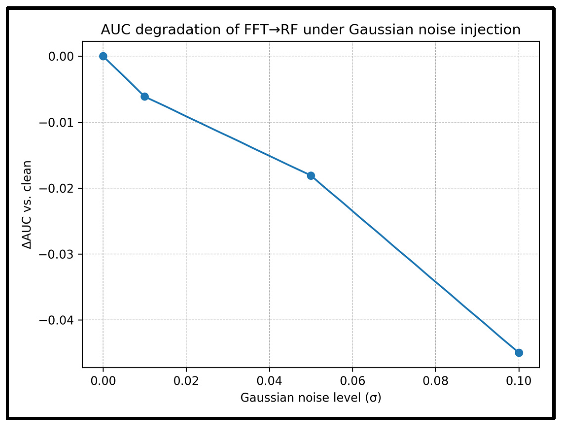
| 16: For each noise level α ∈ Σ and seed k ∈ S: |
| 17: Create Xtest’ = Xtest + N(0, α·std(Xfit)). |
| 18: Compute AUCα, k and Recα, k; aggregate mean ± std; compute Δ vs. clean. |
| 19: On target edge device, benchmark footprint, latency (mean/p50/p95), and peak RSS. |
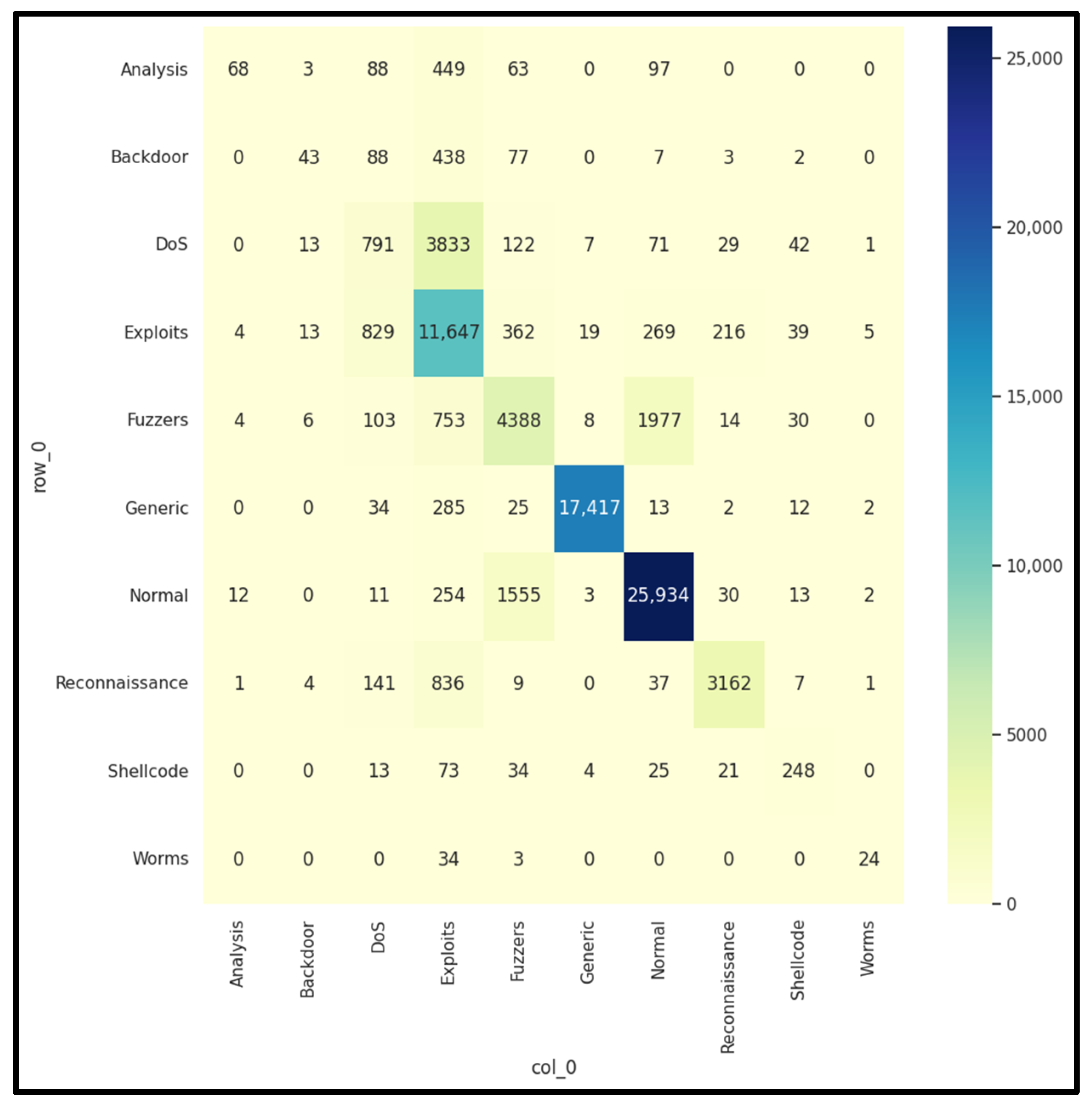
4.8. Final System Validation: Multi-Class Attack Category Detection and Edge Feasibility
5. Conclusions
Author Contributions
Funding
Institutional Review Board Statement
Informed Consent Statement
Data Availability Statement
Conflicts of Interest
References
- Dragusin, S.A.; Bizon, N.; Bostinaru, R.N. Comprehensive Analysis of Cyber-Attack Techniques and Vulnerabilities in Communication Channels of Embedded Systems. In Proceedings of the 16th International Conference on Electronics, Computers and Artificial Intelligence, Iasi, Romania, 27–28 June 2024. [Google Scholar] [CrossRef]
- Dragusin, S.A.; Bizon, N.; Bostinaru, R.N.; Enescu, F.M.; Teodorescu, R.M.; Savulescu, C. Analysis of Vulnerabilities in Communication Channels Using an Integrated Approach Based on Machine Learning and Statistical Methods. In Proceedings of the 16th International Conference on Electronics, Computers and Artificial Intelligence, Iasi, Romania, 27–28 June 2024. [Google Scholar] [CrossRef]
- Borangiu, T.; Morariu, O.; Răileanu, S.; Trentesaux, D.; Leitão, P.; Barata, J. Digital transformation of manufacturing. Industry of the Future with Cyber-Physical Production Systems. Rom. J. Inf. Sci. Technol. 2020, 23, 3–37. [Google Scholar]
- Dragusin, S.; Bizon, N. Emerging Cybersecurity Threats in Embedded Systems: A Review of Attack Techniques, Anomaly Detection, and AI-Based Prediction Approaches. J. Electr. Eng. Electron. Control. Comput. Sci. 2025, 11, 11–22. [Google Scholar]
- Trilles, S.; Hammad, S.S.; Iskandaryan, D. Anomaly detection based on Artificial Intelligence of Things: A Systematic Literature Mapping. Internet Things 2024, 25, 101063. [Google Scholar] [CrossRef]
- Adhikari, D.; Jiang, W.; Zhan, J.; Rawat, D.B.; Bhattarai, A. Recent advances in anomaly detection in Internet of Things: Status, challenges, and perspectives. Comput. Sci. Rev. 2024, 54, 100665. [Google Scholar] [CrossRef]
- Zhang, Y.; Muniyandi, R.C.; Qamar, F. A Review of Deep Learning Applications in Intrusion Detection Systems: Overcoming Challenges in Spatiotemporal Feature Extraction and Data Imbalance. Appl. Sci. 2025, 15, 1552. [Google Scholar] [CrossRef]
- DeMedeiros, K.; Hendawi, A.; Alvarez, M. A Survey of AI-Based Anomaly Detection in IoT and Sensor Networks. Sensors 2023, 23, 1352. [Google Scholar] [CrossRef] [PubMed]
- Morshedi, R.; Matinkhah, S.M. A Comprehensive Review of Deep Learning Techniques for Anomaly Detection in IoT Networks: Methods, Challenges, and Datasets. Eng. Rep. 2025, 7, e70415. [Google Scholar] [CrossRef]
- Reis, M.J.C.S.; Serôdio, C. Edge AI for Real-Time Anomaly Detection in Smart Homes. Future Internet 2025, 17, 179. [Google Scholar] [CrossRef]
- Tahri, R.; Jarrar, A.; Lasbahani, A.; Balouki, Y. A comparative study of Machine learning Algorithms on the UNSW-NB 15 Dataset. In Proceedings of the 4th International Conference on Computing and Wireless Communication Systems, Tangier, Morocco, 21–23 June 2022. [Google Scholar] [CrossRef]
- Rahman, M.; Saad, S.; Satam, P.; Mari, A.-G.; Zinca, D.; Dobrota, V. Development of a Machine-Learning Intrusion Detection System and Testing of Its Performance Using a Generative Adversarial Network. Sensors 2023, 23, 1315. [Google Scholar] [CrossRef] [PubMed]
- Yang, T.; Qiao, Y.; Lee, B. Towards trustworthy cybersecurity operations using Bayesian Deep Learning to improve uncertainty quantification of anomaly detection. Comput. Secur. 2024, 144, 103909. [Google Scholar] [CrossRef]
- Kale, R.; Thing, V.L.L. Few-shot weakly-supervised cybersecurity anomaly detection. Comput. Secur. 2023, 130, 103194. [Google Scholar] [CrossRef]
- Goumidi, H.; Pierre, S. Real-Time Anomaly Detection in IoMT Networks Using Stacking Model and a Healthcare-Specific Dataset. IEEE Access 2025, 13, 70352–70365. [Google Scholar] [CrossRef]
- Kopljar, D.; Drvar, V.; Babic, J.; Podobnik, V. XAAD–Post-Feedback Explainability for Active Anomaly Discovery. IEEE Access 2024, 12, 181914–181924. [Google Scholar] [CrossRef]
- Villarreal-Vasquez, M.; Modelo-Howard, G.; Dube, S.; Bhargava, B. Hunting for Insider Threats Using LSTM-Based Anomaly Detection. IEEE Trans. Dependable Secur. Comput. 2023, 20, 451–462. [Google Scholar] [CrossRef]
- Khan, W.; Ishrat, M.; Ahmed, M.N.; Abidin, S.; Husain, M.; Izhar, M.; Zamani, A.T.; Hussain, M.R.; Ali, A. Enhancing Anomaly Detection in Attributed Networks Using Proximity Preservation and Advanced Embedding Techniques. IEEE Access 2025, 13, 42777–42796. [Google Scholar] [CrossRef]
- Mansourian, P.; Zhang, N.; Jaekel, A.; Kneppers, M. Deep Learning-Based Anomaly Detection for Connected Autonomous Vehicles Using Spatiotemporal Information. IEEE Trans. Intell. Transp. Syst. 2023, 24, 16006–16017. [Google Scholar] [CrossRef]
- Dragusin, S.A.; Bizon, N.; Bostinaru, R.N. A Brief Overview of Current Encryption Techniques Used in Embedded Systems: Present and Future Technologies. In Proceedings of the 15th International Conference on Electronics, Computers and Artificial Intelligence, Bucharest, Romania, 29–30 June 2023. [Google Scholar] [CrossRef]
- Zhang, D.; Feng, G.; Shi, Y.; Srinivasan, D. Physical Safety and Cyber Security Analysis of Multi-Agent Systems: A Survey of Recent Advances. IEEE/CAA J. Autom. Sin. 2021, 8, 319–333. [Google Scholar] [CrossRef]
- Chirilă, A.; Sărăcin, C.; Deaconu, D.; Nicolescu, D.; Radulian, A. Remote monitoring and control system with increased operational technology cybersecurity resilience. UPB Sci. Bull. Ser. C 2024, 86, 223–232. [Google Scholar]
- Nguyen, T.H. Cybersecurity Logging & Monitoring Security Program, DigitalCommons@SHU, Sacred Heart University. School of Computer Science & Engineering Undergraduate Publications, 2022. Available online: https://digitalcommons.sacredheart.edu/computersci_stu/3/ (accessed on 29 January 2025).
- Jing, X.; Yan, Z.; Pedrycz, W. Security data collection and data analytics in the internet: A survey. IEEE Commun. Surv. Tutor. 2019, 21, 586–618. [Google Scholar] [CrossRef]
- Acosta, J.C.; Medina, S.; Ellis, J.; Clarke, L.; Rivas, V.; Newcomb, A. Network Data Curation Toolkit: Cybersecurity Data Collection, Aided-Labeling, and Rule Generation. In Proceedings of the Military Communications Conference, San Diego, CA, USA, 29 November–2 December 2021. [Google Scholar] [CrossRef]
- Shashanka, M.; Shen, M.Y.; Wang, J. User and entity behavior analytics for enterprise security. In Proceedings of the International Conference on Big Data, Washington, DC, USA, 5–8 December 2016. [Google Scholar] [CrossRef]
- Agoramoorthy, M.; Ali, A.; Sujatha, D.; Michael Raj, T.F.; Ramesh, G. An Analysis of Signature-Based Components in Hybrid Intrusion Detection Systems. In Proceedings of the Intelligent Computing and Control for Engineering and Business Systems, Chennai, India, 14–15 December 2023. [Google Scholar] [CrossRef]
- Oppliger, R.; Grunert, A.; Michael, J.B. How to Measure Cybersecurity and Why Heuristics Matter. Computer 2024, 57, 111–115. [Google Scholar] [CrossRef]
- Noble, J.; Adams, N.M. Correlation-Based Streaming Anomaly Detection in Cyber-Security. In Proceedings of the 16th International Conference on Data Mining Workshops, Barcelona, Spain, 12–15 December 2016. [Google Scholar] [CrossRef]
- Dragusin, S.A.; Bizon, N.; Bostinaru, R.N.; Toma, D. Command Recognition System Using Convolutional Neural Networks. In Proceedings of the 16th International Conference on Electronics, Computers and Artificial Intelligence, Iasi, Romania, 27–28 June 2024. [Google Scholar] [CrossRef]
- Lappas, D.; Argyriou, V.; Makris, D. Fourier transformation autoencoders for anomaly detection. In Proceedings of the International Conference on Acoustics, Speech and Signal Processing, Toronto, ON, Canada, 6–12 June 2021. [Google Scholar] [CrossRef]
- Collins Jackson, A.; Lacey, S. Seasonality and Anomaly Detection in Rare Data Using the Discrete Fourier Transformation. In Proceedings of the 1st International Conference on Digital Data Processing, London, UK, 15–17 November 2019. [Google Scholar] [CrossRef]
- Jiang, D.; Zhang, P.; Xu, Z.; Yao, C.; Qin, W. A wavelet-based detection approach to traffic anomalies. In Proceedings of the 7th International Conference on Computational Intelligence and Security, Sanya, China, 3–4 December 2011. [Google Scholar] [CrossRef]
- Golgowski, M.; Osowski, S. Detection of bearing failures using wavelet transformation and machine learning approach. In Proceedings of the International Joint Conference on Neural Networks, Padua, Italy, 18–23 July 2022. [Google Scholar] [CrossRef]
- Thill, M.; Konen, W.; Bäck, T. Online Adaptable Time Series Anomaly Detection with Discrete Wavelet Transforms and Multivariate Gaussian Distributions. Arch. Data Sci. Ser. A 2018, 5, 17. [Google Scholar] [CrossRef]
- Bostinaru, R.N.; Bizon, N.; Dragusin, S.A.; Iana, G.V.; Toma, D. Dimensionality Reduction with Principal Component Analysis for Fire and Non-Fire Audio Classification: A New Approach. In Proceedings of the 17th International Conference on Electronics, Computers and Artificial Intelligence, Targoviste, Romania, 26–27 June 2025. [Google Scholar] [CrossRef]
- Dani, S.K.; Thakur, C.; Nagvanshi, N.; Singh, G. Anomaly Detection using PCA in Time Series Data. In Proceedings of the International Conference on Interdisciplinary Approaches in Technology and Management for Social Innovation, Gwalior, India, 14–16 March 2024. [Google Scholar] [CrossRef]
- Knorn, F.; Leith, D.J. Adaptive Kalman filtering for anomaly detection in software appliances. In Proceedings of the IEEE INFOCOM Workshops, Phoenix, AZ, USA, 13–18 April 2008. [Google Scholar] [CrossRef]
- Ji, I.H.; Lee, J.H.; Kang, M.J.; Park, W.J.; Jeon, S.H.; Seo, J.T. Artificial Intelligence-Based Anomaly Detection Technology over Encrypted Traffic: A Systematic Literature Review. Sensors 2024, 24, 898. [Google Scholar] [CrossRef] [PubMed]
- Zhang, X.; Gu, C.; Lin, J. Support vector machines for anomaly detection. In Proceedings of the 6th World Congress on Intelligent Control and Automation, Dalian, China, 21–23 June 2006. [Google Scholar] [CrossRef]
- Primartha, R.; Tama, B.A. Anomaly detection using random forest: A performance revisited. In Proceedings of the International Conference on Data and Software Engineering, Palembang, Indonesia, 1–2 November 2017. [Google Scholar] [CrossRef]
- Elmrabit, N.; Zhou, F.; Li, F.; Zhou, H. Evaluation of Machine Learning Algorithms for Anomaly Detection. In Proceedings of the International Conference on Cyber Security and Protection of Digital Services, Dublin, Ireland, 15–19 June 2020. [Google Scholar] [CrossRef]
- Kumari Sheetanshu, R.; Singh, M.K.; Jha, R.; Singh, N.K. Anomaly detection in network traffic using K-mean clustering. In Proceedings of the 3rd International Conference on Recent Advances in Information Technology, Dhanbad, India, 3–5 March 2016. [Google Scholar] [CrossRef]
- Ranjith, R.; Athanesious, J.J.; Vaidehi, V. Anomaly detection using DBSCAN clustering technique for traffic video surveillance. In Proceedings of the 7th International Conference on Advanced Computing, Chennai, India, 15–17 December 2015. [Google Scholar] [CrossRef]
- Kiziltas, B.; Gul, E. Network Anomaly Detection with Convolutional Neural Network Based Auto Encoders. In Proceedings of the 28th Signal Processing and Communications Applications Conference, Gaziantep, Turkey, 5–7 October 2020. [Google Scholar] [CrossRef]
- Chen, Z.; Yeo, C.K.; Lee, B.S.; Lau, C.T. Autoencoder-based network anomaly detection. In Proceedings of the Wireless Telecommunications Symposium, Phoenix, AZ, USA, 17–20 April 2018. [Google Scholar] [CrossRef]
- Kumarage, T.; Ranathunga, S.; Kuruppu, C.; De Silva, N.; Ranawaka, M. Generative Adversarial Networks (GAN) based Anomaly Detection in Industrial Software Systems. In Proceedings of the Moratuwa Engineering Research Conference, Moratuwa, Sri Lanka, 3–5 July 2019. [Google Scholar] [CrossRef]
- The UNSW-NB15 Dataset|UNSW Research. Available online: https://research.unsw.edu.au/projects/unsw-nb15-dataset (accessed on 28 October 2025).
- Zhao, Y.; Ma, D.; Liu, W. Efficient Detection of Malicious Traffic Using a Decision Tree-Based Proximal Policy Optimisation Algorithm: A Deep Reinforcement Learning Malicious Traffic Detection Model Incorporating Entropy. Entropy 2024, 26, 648. [Google Scholar] [CrossRef] [PubMed]
- Putrada, A.G.; Alamsyah, N.; Fauzan, M.N.; Oktaviani, I.D. Pearson Correlation for Efficient Network Anomaly Detection with Quantization on the UNSW-NB15 Dataset. In Proceedings of the International Conference on ICT for Smart Society, Bandung, Indonesia, 4–5 September 2024. [Google Scholar] [CrossRef]

| Ref. | Focus/Domain | Techniques/ Models |
Datasets | Evaluation Metrics |
Key Findings/ Limitations |
|---|---|---|---|---|---|
| [5] | TinyML/AIoT anomaly detection on microcontrollers |
CNN, AE, LSTM, DNN, IF, GMM | IMU signals, images, temperature datasets |
Accuracy, F1 | CNN dominant (18.8%). TinyML benefits (latency decreases and privacy increases) but HW/SW heterogeneity and energy reporting limited |
| [6] | IoT layered AD survey | AE, RNN, RBM, CNN, GAN, RL | KDD’99, NSL-KDD, UNSW-NB15, Bot-IoT, CICIDS2017, ADFA, Yahoo Webscope |
Precision, DR, FPR, Accuracy, ROC-AUC, F1 |
Broad taxonomy (physical–network–application); identifies issues of complexity, privacy, interpretability; future XAI and Transformer work |
| [7] | IDS with DL | CNN, RNN, LSTM, GRU, SMOTE, GAN augmentation | CIC-IDS2017, UNSW-NB15 |
Accuracy, DR, Recall for U2R/R2L | Hybrid CNN-RNN improves temporal modeling. imbalance remains issue; calls for cost-sensitive and attention models |
| [8] | AD in IoT and sensor networks | ML and DL hybrids with GNN and attention |
Multiple public IoT datasets | Precision, Recall, F1, ROC (TPR/FPR) |
Highlights trade-off between generality vs. specialization. future work on explainability and energy efficiency |
| [9] | DL for IoT network anomaly detection |
CNN, LSTM, AE, GAN, GNN, Transformer, FL |
CICIDS2017, Bot-IoT, NSL-KDD, TON-IoT |
Accuracy, Precision, Recall, F1 |
DL excels in feature learning. issues with label scarcity and adversarial robustness. advocates FL and XAI |
| [10] | Edge AI for Smart Home IoT | IF + LSTM-AE hybrid, quantized TinyML |
Real and synthetic sensor data | Accuracy, Recall, Latency, Energy use |
Hybrid reduces latency (< 50 ms) on Raspberry Pi. privacy-preserving local inference; future Transformers |
| [11] | ML classifiers on UNSW-NB15 dataset |
DT, NB, KNN, RF, SVM, LR, PSO for features |
UNSW-NB15, NSL-KDD, CICIDS2017 |
Accuracy, Precision, Recall, TPR, TNR, FPR, FNR, FAR | RF most robust; feature selection improves speed and accuracy; ensemble methods recommended |
| [12] | GAN-based IDS robustness testing |
ML classifiers + GAN for adversarial traffic generation |
NSL-KDD | Accuracy, F1, Detection Rate | Adversarial GAN traffic initially bypasses IDS but enhances robustness after retraining; advocates adversarial validation |
| [13] | Uncertainty-aware cybersecurity AD |
BDL, BAE, BVAE | UNSW-NB15, CIC-IDS-2017 |
TPR, FPR, ROC-AUC, F1 | Models aleatoric + epistemic uncertainty; reduces false alerts; integrates uncertainty with XAI for trust |
| [14] | Few-shot/weakly supervised IDS |
Triplet augmentation, MLP, ordinal regression |
NSL-KDD, CIC-IDS2018, TON-IoT |
AUROC, TPR, FPR | High ROC with few labels. scalable to limited annotation settings |
| [15] | IoMT real-time IDS | Stacking ensemble (XGBoost + RF + ANN base models) |
UNSW-NB15 + Healthcare dataset | Accuracy, Precision, Recall, F1, ROC-AUC |
accuracy with low latency; demonstrates value of ensemble learning and domain-specific datasets |
| [16] | Explainable semi-supervised AD | IF + AAD + AWS | Synthetic & real datasets | Accuracy, RMSE of importance scores |
Improves interpretability via feature attributions, bridges active learning and explainable AD |
| [17] | Insider threat detection via LSTM |
LSTM sequence prediction with dynamic top-k selection |
Enterprise EDR logs | TPR, FPR |
FPR. outperforms EDR baselines; suited for high-volume SOC |
| [18] | Attributed network AD with SSL |
GCAE, GCN, GAN, Dual-SVDAE, DVAEGMM |
Cora, Citeseer, BlogCatalog, Flickr |
AUC, AP | Outperforms GCN-AE baselines; strong under noise; shows benefits of adversarial and proximity constraints |
| [19] | CAV IDS | LSTM, ConvLSTM, GNB |
Car Hacking Dataset | Accuracy, F1, Latency | Near-perfect F1 and real-time performance; analyzes memory/latency trade-offs for embedded CAV devices |
| Item | Value |
|---|---|
| 256 flows | |
| 128 flows (50% overlap) |
|
| Number of window-level descriptors per attribute | mean, std, min, max |
| Number of attributes used | 14 |
| 56 | |
| Number of windows | 2012 |
| Window labels | 1695 attack/ 317 normal |
| Technique | Key Settings | Output Feature Type | Measured Runtime | Main Limitation |
|---|---|---|---|---|
| Fourier (DFT/FFT) | Series: spkts_mean; FFT magnitude on window index |
Spectral summaries/band-energy indicators | FFT rfft (2012 windows): per run |
Less informative for strongly non-stationary behavior if used alone |
| Wavelet (CWT/DWT) | Wavelet: Morlet; (CWT) | Multiscale coefficient statistics/energy features | CWT (scales 1–64, Morlet): per run | Parameter sensitivity (wavelet/scales) and higher compute than FFT |
| PCA |
cumulative explained variance (train split). |
Low-dimensional components; explained variance profile | PCA fit performed offline; projection is linear (matrix multiplication) | Linear model; may miss non-linear structure |
| Kalman Filter | 1D model; Q = 10−3, |
Innovation/residual statistics (anomaly-sensitive) | per run | Model/parameter dependence (Q/R, assumptions) |
| Algorithm | Learning Paradigm |
Computational Cost |
Typical Training/ Inference time |
Noise/ Variability Robustness |
Resource Footprint |
Main Limitations | |
|---|---|---|---|---|---|---|---|
| SVM | Supervised | ; inference moderate | Moderate training; fast inference | Moderate (kernel + scaling sensitive) | CPU/RAM moderate | Kernel/parameter sensitivity; scalability issues on large datasets; limited interpretability | |
| RF | Supervised (ensemble) |
baseline; robust decision rules for heterogeneous tabular descriptors; -depth) | Fast training; fast inference | High (stable under feature noise/variance) | Model size may grow; less efficient than boosting when heavily tuned; limited calibrated probabilities | ||
| XGBoost | Supervised (boosting) | Training higher than RF; inference |
Moderate training; fast inference | High (with regularization) | CPU/RAM moderate | Sensitive to hyperparameters; risk of overfitting without careful regularization | |
| LightGBM | Supervised (boosting) | Efficient training; inference |
Moderate training; fast inference | High (often robust on engineered descriptors) | CPU/RAM moderate | Parameter-sensitive; performance depends on tuning and handling class imbalance | |
| K-Means | Unsupervised (clustering) |
per iteration |
Fast training/inference | Low–Moderate | Low | Requires k; sensitive to initialization and feature scaling; weak on irregular cluster shapes | |
| DBSCAN | Unsupervised (density-based) |
; isolates sparse regions as anomalies; Often with indexing (data-dependent) |
Moderate | Moderate–High (good at isolating sparse outliers) | CPU moderate |
Sensitive to ; degrades in high-dimensional spaces; unstable under varying density |
|
| AE | DL, reconstruction-based) |
Training depends on architecture/epochs; inference low–moderate | Moderate training; fast inference | High (if trained on “normal” distribution; benefits from denoising) | CPU/GPU depending on architecture | Requires careful training protocol; thresholding/calibration needed; can reconstruct some attacks (missed anomalies) | |
| GAN | DL, distribution-based |
Training expensive/unstable; inference moderate | High training cost; inference moderate | High in principle, but depends strongly on stable training | Typically, GPU for training | Training instability (mode collapse); sensitive to hyperparameters; harder to reproduce consistently | |
| Inference Rate f |
Window Duration |
Latency Budget |
Headroom Latency |
|
|
|
|
|---|---|---|---|---|---|---|---|
| Model | Acc | Prec | Rec | F1 | AUC |
|---|---|---|---|---|---|
| SVM | 0.9949 | 0.9999 | 0.9939 | 0.9969 | 0.9999 |
| RF | 0.9974 | 0.9970 | 0.9999 | 0.9985 | 0.9999 |
| XGBoost | 0.9949 | 0.9969 | 0.9969 | 0.9969 | 0.9999 |
| LightGBM | 0.9974 | 0.9970 | 0.9999 | 0.9985 | 0.9998 |
| K-Means proxy (k = 2) | 0.8385 | 0.8385 | 0.999 | 0.9121 | 0.2312 |
| K-Means one-class (k = 5, p95) | 0.9769 | 0.9818 | 0.9908 | 0.9863 | 0.9965 |
| K-Means one-class (k = 5, p97) | 0.9718 | 0.9877 | 0.9786 | 0.9831 | 0.9965 |
| K-Means one-class (k = 5, p99) | 0.9615 | 0.9906 | 0.9633 | 0.9767 | 0.9965 |
| DBSCAN one-class (p95) | 0.8359 | 0.9999 | 0.8043 | 0.8915 | 0.9224 |
| DBSCAN one-class (p97) | 0.8282 | 0.9999 | 0.7951 | 0.8859 | 0.9224 |
| DBSCAN one-class (p99) | 0.7897 | 0.9999 | 0.7492 | 0.8566 | 0.9224 |
| AE one-class (p95) | 0.9769 | 0.9732 | 0.9999 | 0.9864 | 0.9999 |
| AE one-class (p97) | 0.9821 | 0.9790 | 0.9999 | 0.9894 | 0.9999 |
| AE one-class (p99) | 0.9949 | 0.9999 | 0.9939 | 0.9969 | 0.9999 |
| GAN one-class (p95) | 0.9949 | 0.9969 | 0.9969 | 0.9969 | 0.9999 |
| GAN one-class (p97) | 0.9923 | 0.9999 | 0.9908 | 0.9954 | 0.9999 |
| GAN one-class (p99) | 0.9923 | 0.9999 | 0.9908 | 0.9954 | 0.9999 |
| Model | Acc | Prec | Rec | F1 | AUC |
|---|---|---|---|---|---|
| SVM | 0.9872 | 0.9847 | 0.9961 | 0.9904 | 0.9994 |
| RF | 0.9821 | 0.9773 | 0.9961 | 0.9866 | 0.9988 |
| XGBoost | 0.9897 | 0.9885 | 0.9961 | 0.9923 | 0.9996 |
| LightGBM | 0.9949 | 0.9923 | 0.9999 | 0.9962 | 0.9999 |
| K-Means proxy (k = 2) | 0.6282 | 0.7021 | 0.7645 | 0.7320 | 0.6026 |
| K-Means one-class (k = 5, p95) | 0.7231 | 0.9521 | 0.6139 | 0.7465 | 0.8979 |
| K-Means one-class (k = 5, p97) | 0.5974 | 0.9811 | 0.4015 | 0.5699 | 0.8979 |
| K-Means one-class (k = 5, p99) | 0.5410 | 0.9762 | 0.3166 | 0.4781 | 0.8979 |
| DBSCAN one-class (p95) | 0.8564 | 0.9721 | 0.8069 | 0.8819 | 0.9753 |
| DBSCAN one-class (p97) | 0.8205 | 0.9846 | 0.7413 | 0.8458 | 0.9833 |
| DBSCAN one-class (p99) | 0.7385 | 0.9999 | 0.6062 | 0.7548 | 0.9894 |
| AE one-class (p95) | 0.9308 | 0.9085 | 0.9961 | 0.9503 | 0.9882 |
| AE one-class (p97) | 0.9538 | 0.9547 | 0.9768 | 0.9656 | 0.9882 |
| AE one-class (p99) | 0.9282 | 0.9793 | 0.9112 | 0.9440 | 0.9882 |
| GAN one-class (p95) | 0.8103 | 0.9602 | 0.7452 | 0.8391 | 0.9612 |
| GAN one-class (p97) | 0.7231 | 0.9809 | 0.5946 | 0.7404 | 0.9612 |
| GAN one-class (p99) | 0.7000 | 0.9863 | 0.5560 | 0.7111 | 0.9612 |
| Model | Acc | Prec | Rec | F1 | AUC |
|---|---|---|---|---|---|
| SVM | 0.9231 | 0.9167 | 0.9742 | 0.9445 | 0.9444 |
| RF | 0.9901 | 0.9926 | 0.9926 | 0.9926 | 0.9995 |
| XGBoost | 0.9926 | 0.9963 | 0.9926 | 0.9945 | 0.9993 |
| LightGBM | 0.9926 | 0.9963 | 0.9926 | 0.9945 | 0.9998 |
| K-Means proxy (k = 2) | 0.9181 | 0.9103 | 0.9742 | 0.9412 | 0.4192 |
| K-Means one-class (k = 5, p95) | 0.9107 | 0.9681 | 0.8967 | 0.9310 | 0.9705 |
| K-Means one-class (k = 5, p97) | 0.8189 | 0.9670 | 0.7565 | 0.8489 | 0.9705 |
| K-Means one-class (k = 5, p99) | 0.7494 | 0.9670 | 0.6494 | 0.7770 | 0.9705 |
| DBSCAN one-class (p95) | 0.5434 | 0.9579 | 0.3358 | 0.4973 | 0.9888 |
| DBSCAN one-class (p97) | 0.4591 | 0.9492 | 0.2066 | 0.3394 | 0.9888 |
| DBSCAN one-class (p99) | 0.3871 | 1.0000 | 0.0886 | 0.1627 | 0.9888 |
| AE one-class (p95) | 0.9752 | 0.9711 | 0.9926 | 0.9818 | 0.9956 |
| AE one-class (p97) | 0.9801 | 0.9852 | 0.9852 | 0.9852 | 0.9956 |
| AE one-class (p99) | 0.9777 | 0.9888 | 0.9779 | 0.9833 | 0.9956 |
| GAN one-class (p95) | 0.9677 | 0.9674 | 0.9852 | 0.9762 | 0.9953 |
| GAN one-class (p97) | 0.9801 | 0.9852 | 0.9852 | 0.9852 | 0.9953 |
| GAN one-class (p99) | 0.9801 | 0.9852 | 0.9852 | 0.9852 | 0.9953 |
| Model | Acc | Prec | Rec | F1 | AUC |
|---|---|---|---|---|---|
| SVM | 0.9954 | 0.9933 | 1.0000 | 0.9967 | 0.7494 |
| RF | 0.9890 | 0.9919 | 0.9919 | 0.9919 | 0.8028 |
| XGBoost | 0.9963 | 0.9960 | 0.9987 | 0.9973 | 0.7785 |
| LightGBM | 0.9945 | 0.9933 | 0.9987 | 0.9960 | 0.7898 |
| K-Means | 0.9314 | 0.9539 | 0.9449 | 0.9494 | 0.5002 |
| DBSCAN | 0.2957 | 0.3866 | 0.4756 | 0.4265 | 0.2812 |
| AE | 0.8719 | 0.8784 | 0.9422 | 0.9092 | 0.5724 |
| GAN | 0.8454 | 0.8468 | 0.9435 | 0.8926 | 0.4344 |
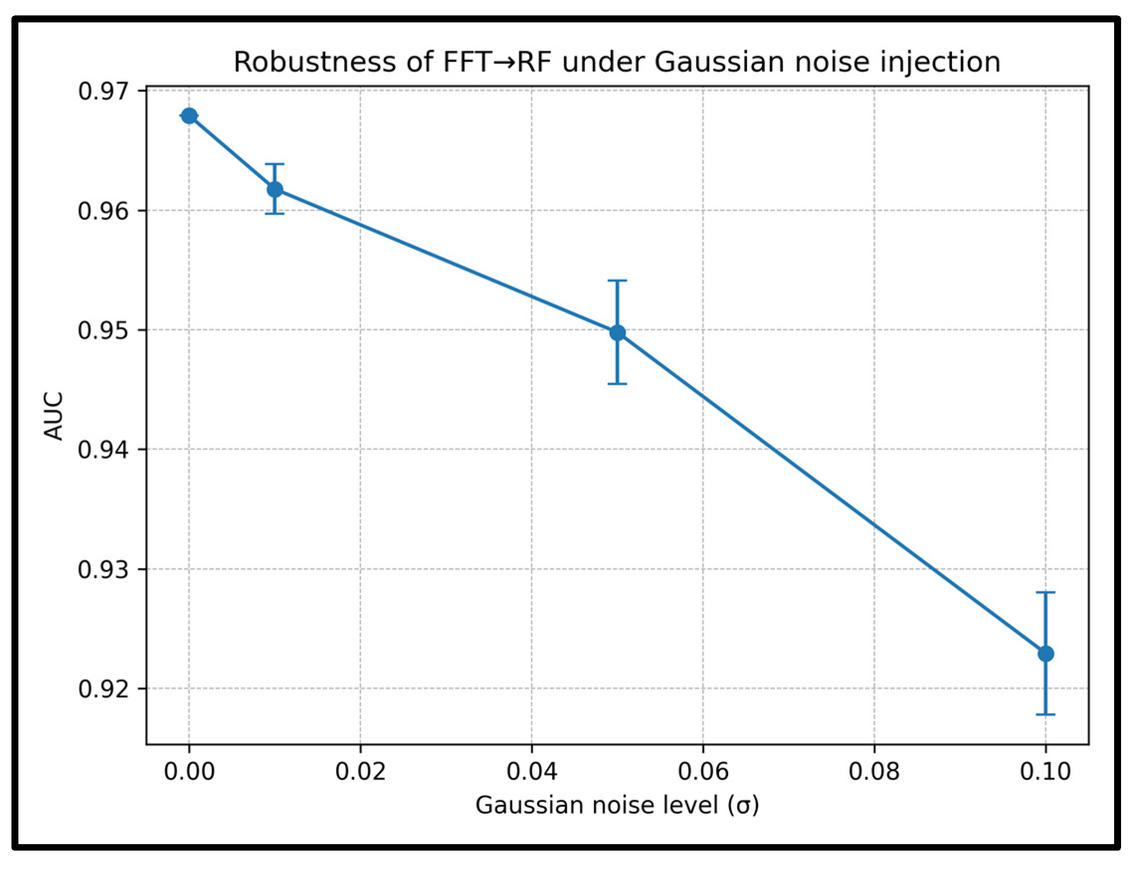
| Gaussian Noise Level (σ) | AUC (Mean ± Std) |
ΔAUC vs. Clean |
Recall (Mean ± Std) |
ΔRecall vs. Clean |
|---|---|---|---|---|
| 0.00 | 0.9679 ± 0.0000 | 0.0000 | 0.9186 ± 0.0000 | 0.0000 |
| 0.01 | 0.9618 ± 0.0021 | −0.0061 | 0.9093 ± 0.0028 | −0.0092 |
| 0.05 | 0.9498 ± 0.0043 | −0.0181 | 0.9015 ± 0.0050 | −0.0171 |
| 0.10 | 0.9229 ± 0.0051 | −0.0450 | 0.8903 ± 0.0033 | −0.0283 |
| Representation Module |
Feature Dim. |
Acc | Prec | Rec | F1 | AUC | Key Interpretation |
|---|---|---|---|---|---|---|---|
| FFT + RF | Best overall trade-off for deployment: near-ceiling detection with predictable sliding-window runtime and explicit feasibility envelope. | ||||||
| DWT + RF | Strong AUC/recall but lower accuracy than FFT; best treated as offline/selectively enabled when transient localization is needed. | ||||||
| Kalman + RF | Excellent performance with very low feature dimension; attractive for tight memory/compute budgets where “spectral richness” is not required. | ||||||
| PCA + RF | PCA is best positioned as compact/interpretability support and anomaly visualization; not the primary discriminative driver compared to FFT/Kalman in the final embedded framework. |
| Attack Type |
Accuracy % |
Precision % |
Recall % |
F1 % |
Specificity % |
|---|---|---|---|---|---|
| Reconnaissance | 99.48 | 99.51 | 98.23 | 98.86 | 99.86 |
| Analysis | 98.53 | 97.44 | 98.50 | 97.97 | 98.55 |
| DoS | 96.74 | 84.45 | 79.90 | 82.11 | 98.48 |
| Backdoor | 97.86 | 84.05 | 74.98 | 79.26 | 99.18 |
| Fuzzers | 90.06 | 69.14 | 77.04 | 72.87 | 92.79 |
| Shellcode | 99.52 | 61.03 | 55.91 | 58.36 | 99.78 |
| Worms | 99.94 | 68.97 | 33.90 | 45.45 | 99.99 |
| Exploits | 91.96 | 36.65 | 36.23 | 36.44 | 95.75 |
| Normal | 98.80 | 32.82 | 16.29 | 21.77 | 99.65 |
| Generic | 98.80 | 23.97 | 15.90 | 19.11 | 99.54 |
Disclaimer/Publisher’s Note: The statements, opinions and data contained in all publications are solely those of the individual author(s) and contributor(s) and not of MDPI and/or the editor(s). MDPI and/or the editor(s) disclaim responsibility for any injury to people or property resulting from any ideas, methods, instructions or products referred to in the content. |
© 2025 by the authors. Licensee MDPI, Basel, Switzerland. This article is an open access article distributed under the terms and conditions of the Creative Commons Attribution (CC BY) license (http://creativecommons.org/licenses/by/4.0/).


