Submitted:
22 December 2025
Posted:
23 December 2025
You are already at the latest version
Abstract
We consider two steady state heat conduction systems called, S and Sα, in a multidimensional bounded domain D for the Poisson equation with source energy g. In one system we impose mixed boundary conditions (temperature b on the boundary Γ1, heat flux q on Γ2 and an adiabatic condition on Γ3). In the other system, the condition on Γ1 is replaced by a convective heat flux condition with coefficient α. For each of these systems, we consider three associated optimization problems (Pi) and (Piα), i = 1, 2, 3 where the variable will be the source energy g, the heat flux q and the environmental temperature b, respectively. In the particular case that D is a rectangle, the explicit continuous optimization variables and the corresponding state of the systems are known. In the present work, by using a finite difference scheme, we obtain the discrete systems (Sh) and (Sh α) and discrete optimization problems (Pih) and (Pihα), i = 1, 2, 3, where h is the space step in the discretization. Explicit discrete solutions are found, and convergence and estimation errors results are proved when h goes to zero and when α goes to infinite. Moreover, some numerical simulations are provided in order to test theoretical results. Finally, we note that the use of a three–point finite–difference approximation for the Neumann or Robin boundary condition at the boundary improves the global order of convergence from O(h) to O(h2).
Keywords:
optimal control
; finite difference method
; explicit discrete solutions
; estimation error
1. Introduction
We consider a multidimensional bounded domain whose regular boundary consists of three disjoint portions with for . We define two stationary heat conduction problems and with mixed boundary conditions which are given by (1)-(2) and (1)-(3) respectively:
where g is the internal energy of the system in , the environmental temperature on , q is the heat flux on and is the convective heat coefficient on We assume that: , and These problems can be considered as Stefan’s stationary problems [8,19,20,21,22]. Notice that mixed boundary conditions play an important role in several applications, e.g. heat conduction and electric potential problems [12].
The variational formulation of the elliptic problems (1)-(2) and (1)-(3) can be found in [8,9,10,19]. It can be seen that they have unique solution [20]. In general, the solutions of mixed elliptic boundary problems is not so regular [11] but there are cases in which they are regular [4,15,18]. Other theoretical optimization problems in the subject have been done in [13,25].
We define the optimization problems and , associated to the systems and , respectively (see [5,9,16,17,24]).
The distributed optimization problems and on the constant internal energy g are formulated as:
where and are given by
with and . For each , the functions and denote the unique solutions to the systems and respectively, for data , .
The boundary optimization problems and on the constant heat flux q on are defined as:
where and are given by
with and . For each , we denote with and the unique solutions to the systems and respectively, for data and .
The boundary optimization problems and on the constant temperature b in an external neighborhood of are set as
where and , given by
with and . For every , the functions and are the unique solutions of the systems and respectively, for data and , .
In [6] the explicit solutions to the continuous systems and were obtained, as well as the associated optimization problems and for , in the particular case when the domain is a rectangle. These explicit solutions provide a benchmark for testing the accuracy of numerical methods.
The goal of this paper is to find the discrete explicit solutions to the systems and , through the finite difference method, in a rectangular domain. In addition, we aim to obtain the discrete explicit solutions to the optimization problems and for . Taking advantage of the exact explicit solutions, we will estimate the order of convergence of the approximate solutions as a function of the step discretization.
It is worth to mention that there are several articles available in the literature that obtain explicit discrete solutions of some optimization problems [1,2,3]. For example, in [14], exact formulas are derived for the solution of an optimal boundary control problem governed by the one dimensional heat equation where the control function measures the distance of the final state from the target. In [26] a finite element approximation is applied for some kind of parabolic optimal control problems with Neumann boundary conditions. Some numerical experiments are carried out setting a rectangular domain.
This paper is organized as follows: in Section 2 we obtain the discrete explicit solution to the systems and by the finite difference method. In Section 3, we obtain explicit discrete solutions to the discrete distributed optimization problems associated to and , respectively where the variable is the internal energy g. In Section 4, we define discrete boundary optimization problems where the variable is the heat flux q, associated to and , respectively obtaining the discrete explicit solutions. In the same manner, in Section 5, we derive explicit discrete solutions to the discrete boundary optimal control problems associated to and , respectively where the optimization variable is b. In all cases, when the step discretization goes to zero, convergence results are obtained estimating also the order of convergence of the approximate solutions. In Section 6, we carry out some numerical simulations in order to illustrate the convergence theoretical results obtained in the previous sections. Finally, in Section 7, we analyze the order of convergence of the discrete systems associated with and by considering a modified approximation of the Neumann boundary condition on , which leads to an improved convergence order.
2. Discrete Systems for and
In this section we obtain the discrete explicit solutions to the systems and in a particular domain.
Let us consider a rectangular domain in the plane with and . Its boundaries for are defined by:
and
According to [6] the continuous solutions, in , for the systems and defined by (1)-(2) and (1)-(3) are given by:
As consequence of the symmetry of the domain , the solution u and of the systems and are independent of the variable y, and therefore we will work with one-dimensional problems.
Given , we define:
where, n is the number of subintervals to consider in , h is the constant size of these subintervals, and is the approximate value of the function u in for .
We apply the classical finite–difference method to the system described by equations (1)–(2). Since the boundary condition on prescribes , we immediately obtain .
For the interior nodes, we use the classical centered second–order finite difference approximation:
and from (1) it follows that
To incorporate the Neumann boundary condition on , we use a backward finite difference for the first derivative:
which, using the boundary condition , leads to
As a consequence, we obtain the discrete linear system
where is the vector of unknowns, A is the associated tridiagonal coefficient matrix:
and is the vector of independent terms:
The square matrix A is invertible and its inverse matrix is given by
Then the system has a unique solution:
As , it follows that:
Then, the continuous solution of system can be approximated by the piecewise linear interpolant obtained from the nodal values computed by the finite difference scheme. More precisely, we define
with
In the following lemma, we give some bounds for the approximate function
Lemma 1.
- a)
-
For every with , , we have that:
- i)
- if then .
- ii)
- if then .
- b)
-
The following bounds hold:where and
Proof.
- a)
- From functions u and , we have that
- b)
The norm can be computed analogously.
□
We apply the classical finite–difference method to the system defined by equations (1)–(3) where for .
The Robin boundary condition on is approximated by a forward finite–difference scheme, namely,
Moreover, at the interior nodes we use the approximation given in (16), while the Neumann boundary condition at is discretized according to (17).
Then we obtain a linear system :
where the vector of unknowns is given by , the tridiagonal coefficient matrix of order , is defined as:
and
It can be seen that the square matrix is invertible and its inverse matrix is given by
Then the linear system has a unique solution:
As a consequence, the continuous solution of the system , can be approximated by the discrete function in given by
for ,
Notice that , when for each . In addition, when for every .
Lemma 2.
If is the solution of and is the function given in (26) for each h, it follows that:
with and
Proof.
From the definition of and , we have
In addition, the derivatives of the functions and are given by:
and
Then, the bound for coincides with the bound for , obtained in Lemma 21. □
Remark 1.
Notice that when , where is given in Lemma 21.
3. Distributed Optimization Problem with Variable g
In this section we are going to obtain discrete optimal solutions to the continuous optimization problem and in the rectangular domain for the case when the optimization variable is g.
3.1. Discrete Problem Associated to
Taking into account that and the desired state are constants in the expression (6), according to [6], the continuous quadratic functional cost for the problem is explicitly given by:
Since the function is a polynomial function of the variable g, the analytic expresssion for is given by
Then, the continuous solution to the distributed optimization problem is defined by:
and the continuous optimization state is
We define the discrete distributed optimization problem on the constant internal energy g as
where the discrete cost function is given by:
with h defined in (14) and given in (22).
Taking into account that the variable g is constant it results that:
and from algebraic work it follows that
Lemma 3.
The following estimate holds
where does not depend on
Since the function is a polynomial function of the variable g, it is easy to obtain the following analytic expression for the function :
From the optimality condition we obtain the following result:
Lemma 4.
- a)
-
The explicit expression for the optimal variable is given by:where
- b)
-
In addition, the following error estimates hold:where and do not depend on h.
Proof.
- a)
- It follows immediately from the expression of given by (34).
- b)
-
From the expression for with and with , it results that:
□
Lemma 5.
Let us consider the solution of (1)-(2) for and the discrete solution defined as in (22) for , where is the optimal variable of given by (35). We have that:
where and are positive constants independent of the parameter
Proof:
3.2. Discrete Problem Associated to
From [6], we know that the continuous quadratic functional cost in (6) for the optimization problem is explicitly given by:
where is defined by (27). Moreover, the continuous optimal distributed variable denoted by is
The continuous associated state is established by:
Defining the discrete cost function as:
where the function is given in (26) we set the following discrete optimization problem on the constant internal energy g as
The discrete cost function is explicitly given by
where is given by (40).
Lemma 6.
For and the following estimate holds
with
a constant independent of
Proof.
It follows immediately from expression (44). □
Remark 2.
when , where is given in Lemma 3.
Lemma 7.
- a)
-
The explicit expression for the optimal variable is given by:where
- b)
-
In addition, the following error estimates hold:where and do not depend on h.
Proof.
- a)
- It follows immediately from the fact that
- b)
-
Following Lemma 4 it is obtained formula (48) with
□
Remark 3.
Lemma 8.
Let us consider the function given by (14) for where is the optimal variable of problem given by (41) and the function defined by (26) for where is the optimal variable of given by (35). We have that:
where and are positive constants independent of the parameter
Proof.
Remark 4.
and when where and are given in Lemma 5.
Remark 5.
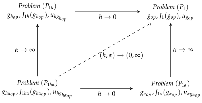
In [23] the double convergence when of the optimal control problem has been studied, obtaining a commutative diagram that relates the continuous and discrete optimal control problems , , and as in the following scheme:
4. Boundary Optimization Problem with Variable q
4.1. Discrete Problem Associated to
Under the same considerations given in Section 3.1 and taking into account formula (9), for a given , we obtain the following quadratic cost function:
Then, the boundary optimal control of the problem , called , and the associated continuous optimal state are given by:
Associated to , we define the approximate discrete distributed optimal control problem on the constant heat flux q as
where the discrete cost function is defined by
where is given in (22), h is the spatial step, and (the desired state) and the control q are constant. From the definition of norm over Q, it results that:
and working algebraically, we get
Lemma 9.
Given and , we have that
where is a constant independent of
proof: It follows immediately from the expression (52) for .
Lemma 10.
Let us consider
- a)
-
The explicit expression for the optimal variable is given by:with
- b)
-
The following error estimates hold:where and are constants independent of h.
Proof.
□
4.2. Discrete Problem Associated to
If we suppose that the desired state is constant in (9), the quadratic cost function for the optimal control problem is explicitly given by:
where
Then, the continuous boundary optimization control, called , and the associated state are:
Remark 6.
Notice that for all and when .
Defining the discrete cost function as:
where is the solution of given in (26), we set the following discrete optimization problem on the constant heat flux q as
Working algebraically, the cost function can be written explicitly as:
Lemma 12.
For each and , we have that:
with
a constant independent of
Proof.
It follows immediately from expression (65). □
Lemma 13.
Let us consider
- a)
-
The explicit expression for the optimal control is given by:with
- b)
-
The following error estimates hold:where and does not depend on h.
Proof.
□
Lemma 14.
Proof.
Similarly to what was done in Lemma 12 it is obtained that
□
Remark 7.
The constants verify that , when for each
Remark 8.
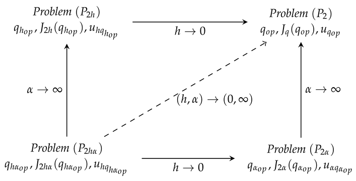
The double convergence when of the optimal control of the problem holds. The relationship of the optimal control problems , , and is given by the following diagram:
5. Boundary Optimization Problem with Variable b
5.1. Discrete Problem Associated to
In this section we consider the boundary optimal control problem given by (10). Taking into account expression (12), for a given constant b we get that
Then the boundary optimal variable of the problem , called , and the associated continuous optimal state, are given respectively by:
We define the discrete optimal control problem on the constant temperature b as
where the discrete cost function is defined as:
where is given in (22), h is the spatial step, and (the desired state) is constant.
Notice that the cost function can be explicitly written as:
Lemma 15.
Let and we have that:
where
does not depend on
Proof.
It follows from expression (75) for . □
Lemma 16.
Let us consider .
- a)
- The explicit expression for the optimal variable is given by:
- b)
-
The following error estimates hold:where and do not depend on h.
Proof.
□
Lemma 17.
Let us consider the solution of (1) -(3) for and the discrete solution given in (26) for and Then we have that:
where and are constants that do not depend on h.
Proof.
Working algebraically it is obtained that
Then it is obtained estimate with
In a similar manner we get that estimate holds with
□
5.2. Discrete Problem Associated to
From [6], we know that the continuous quadratic functional cost in (6) for the optimization problem is explicitly given by:
where is defined by (73). Moreover, the continuous optimal boundary control is given by
The continuous associated state is established by:
Defining the discrete cost function as:
where is the solution of given in (26), we set the following discrete optimization problem as
Working algebraically lead us to write as follows:
Lemma 18.
For and we have that
with
Proof.
It arises immediately from (86). □
Lemma 19.
Let us consider .
- a)
-
The explicit expression for the optimal control is given by:where is given in (77).
- b)
-
The following error estimates hold:where and do not depend on h.
Proof.
□
Lemma 20.
Proof.
Similarly to what was done in Lemma 12 it is obtained that
□
Remark 9.
The constants obtained in the estimates of the previous lemmas verify that , when for .
Remark 10.
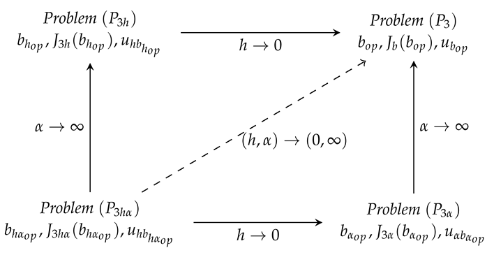
The double convergence when of the optimal control of the problem holds. The relationship of the optimal control of the problems , , and is given by the following diagram:
6. Numerical Results
We will carry out some numerical simulations in order to illustrate the theoretical results obtained in the previous sections for the optimal control problems and for .
Throughout this section we consider the domain , i.e, .
Before analyzing the optimal control problems we illustrate the behavior of the continuous state of the systems and and the discrete state of the systems and .
In Figure 1 a) we plot the state of the system u given by (13) and the approximate discrete function defined by (22) against the position x for . As we saw in Lemma 1 for each fixed x, the increase and get closer to the limit as h decreases. In a similar manner, in Figure 1 b), for we obtain the system given by (13) and the approximate discrete function defined by (26) against the position x for . Notice that as h decreases, the functions increase and get closer to the limit as it was proved in Lemma 2.
In addition in order to visualize the double convergence of when , in Figure 2 we plot u and for and .
6.1. Control Variable g
In this subsection we obtain some computational examples for the optimal distributed control problems , , and . For each plot we set and .
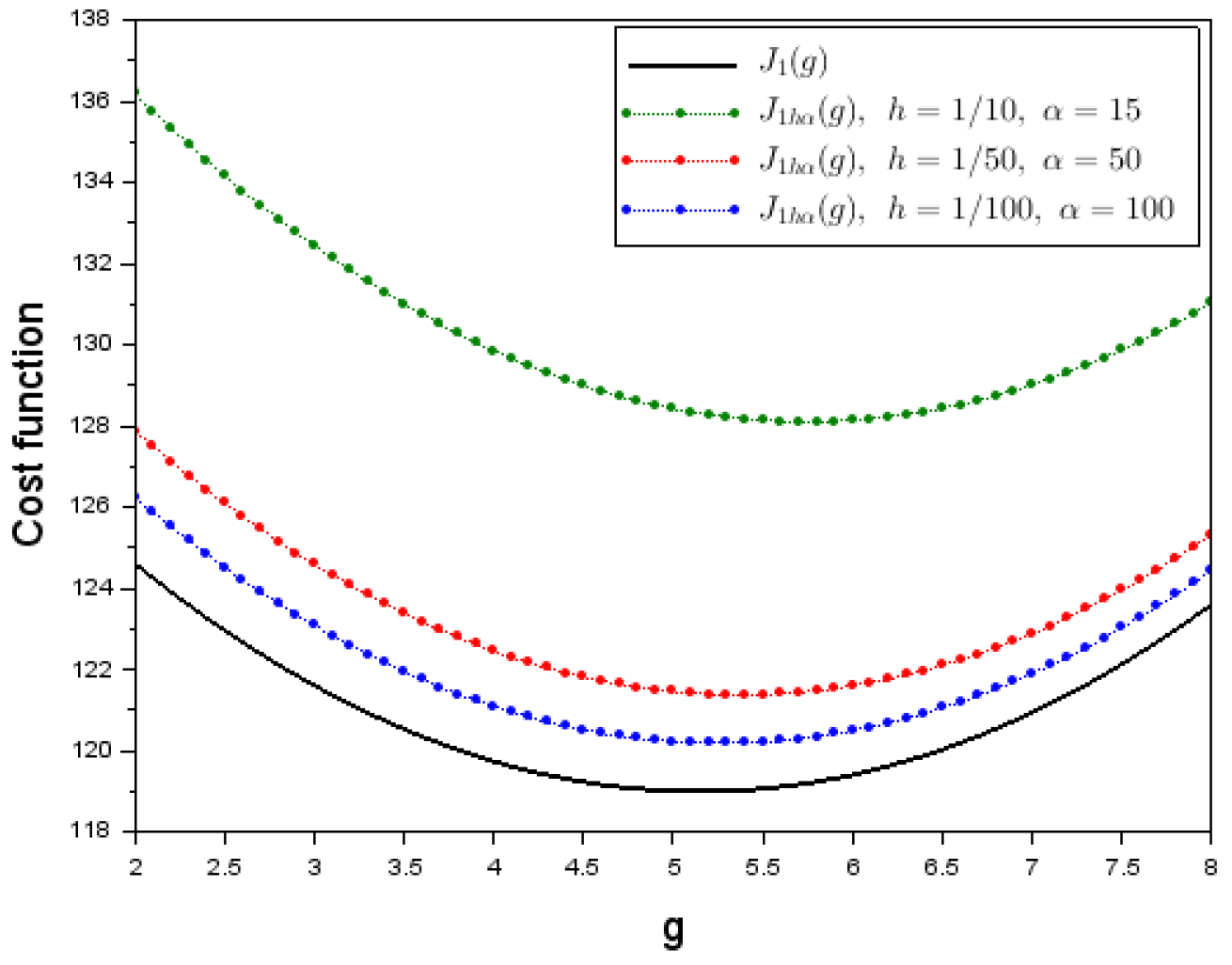
In Figure 3 we plot the continuous quadratic cost function given by (27) and the discrete cost function obtained in (32) against g for , and . Notice that as h decreases the function also decreases to the limit function in agreement with Lemma 3. In a similar manner in Figure 3, for we obtain the continuous function and the discrete functions for and observing the convergence of as h decreases to 0. Moreover, Figure 3 shows the double convergence of when . We illustrate how gets closer to as the value of h decreases and the value of increases.
In Figure 3 we plot the continuous optimal control for the problem given by (29) and the optimal control given by (41) for . Notice that as increases, decreases to the limit . In addition, we set different values of n between and . Recalling that , for each h we obtain the optimal discrete control to the problem defined by (4) and the optimal discrete control to the problem given by (41) for . For each fixed, we have that the discrete solution when , i.e. .
6.2. Control Variable q
In this subsection we run some computational examples for the optimal boundary control problems , , and . For each plot we set and .
In Figure 4 we plot the continuous quadratic cost function given by (50) and the discrete cost function obtained in (52) against q for , and . Observe that as h decreases the function also decreases to the limit function . In a similar way, in Figure 4, for we obtain the continuous function and the discrete functions for and . The convergences and when are in agreement with Lemmas 9 and 12, respectively.
Moreover, Figure 4 shows the double convergence of when . We illustrate how gets closer to as the value of h decreases and the value of increases.
In Figure 4 we plot the continuous optimal control for the problem given by (51) and the optimal control given by (63) for . Notice that as increases, decreases to the limit . In addition, we set different values of n between and . Recalling that , for each h we obtain the optimal discrete control to the problem defined by (54) and the optimal discrete control to the problem given by (67) for . For each fixed, we have that the discrete solution when , i.e. .
6.3. Control Variable b
In this section we obtain some computational examples for the optimal distributed control problems , , and . For each plot we set and .
In Figure 5 we plot the continuous quadratic cost function given by (73) and the discrete cost function obtained in (75) against g for , and . Notice that as h decreases the function also decreases to the limit function in agreement with Lemma 15. In a similar manner in Figure 5, for we obtain the continuous function and the discrete functions for and . Observe the convergence of as . Moreover, Figure 5 shows the double convergence of when . We illustrate how gets closer to as the value of h decreases and the value of increases.
In Figure 5 we plot the continuous optimal control for the problem given by (74) and the optimal control given by (83) for . Notice that as increases, decreases to the limit . In addition, we set different values of n between and . Recalling that , for each h we obtain the optimal discrete control to the problem defined by (77) and the optimal discrete control to the problem given by (88) for . For each fixed, we have that the discrete solution decreases to when .
7. Improvement of the Order of Convergence
In this section, we introduce alternative discrete solutions and associated with the systems and , respectively, and analyze the order of convergence of to u and of to as . The Neumann boundary condition on is approximated by a three–point backward finite–difference scheme. Moreover, for the discrete solution , the Robin boundary condition on is approximated by a three–point forward finite–difference scheme. These higher–order boundary approximations lead to an improved order of accuracy.
We consider the system defined by equations (1)–(2). From this system, we define the discrete problem , where approximates , for . Notice that, from the Dirichlet condition on it follows immediately that .
For the interior nodes, we employ the classical centered second–order finite–difference approximation given in (15), which leads to the discrete system (16) for , .
For the Neumann boundary condition on , we use the three–point backward approximation
Thus, the discrete Neumann condition can be written as
In addition, from (16) for , we obtain
Subtracting the two previous equations, it follows that
Therefore the system given by (16) together with (95) can be written as
where is the vector of unknowns, A is the matrix given by (20) and is the vector of independent terms:
Notice that the system (96) differs from (19) in the last component of the vector of independent terms. Solving the linear system gives
Taking into account that for
and
the linear approximation is given by , i.e.
In the following lemma, we give some bounds for the approximate function
Lemma 21.
The following bounds hold:
where and .
Proof.
From the definition of the norm in the space H and using the expressions (13) and (101) for the functions u and , respectively, it follows that
where
Note that, within each subinterval, depends only on x and the index i, but not on y, since both u and are constant along the y-direction.
A direct computation yields
Then
In addition,
where
for . Then
□
Remark 11.
We emphasize that by improving the approximation of the Neumann boundary condition on , the convergence order of the error is increased to second order, namely . This enhancement leads to a more accurate numerical approximation while remaining fully consistent with the theoretical convergence results established in [7,13].
Remark 12.
The linear system (96) obtained by using the three–point backward finite–difference approximation for the Neumann boundary condition on can be equivalently interpreted by introducing a ghost point outside the computational domain and assuming that the discrete differential equation holds at the boundary node . Indeed, assuming that the equation is satisfied at , we have
while the Neumann boundary condition is approximated by
Eliminating the ghost value from these two expressions yields
which coincides with the boundary equation obtained in (95). Hence, the three–point backward finite–difference approximation of the Neumann condition is consistent with the ghost–point formulation and leads to the same discrete system.
Analogously to the analysis of system , we propose a new discrete approximation for system and study the order of convergence of to as . The associated discrete system employs a three–point backward finite–difference approximation for the Neumann boundary condition on and a three–point forward finite–difference approximation for the Robin boundary condition on , leading to improved accuracy.
We consider the system defined by equations (1)–(3) and define .
For the interior nodes, , we employ the classical centered second–order finite–difference approximation given in (15):
For the Robin boundary at , we use the three–point forward approximation:
Combining this expression with the interior equation at yields the simplified discrete condition
For the Neumann boundary at we use the three–point backward approximation:
Combining with the interior equation for gives
The system given by (106), (108) and (110) can be rewritten as
where is the vector of unknowns, is the matrix given by (24) and is the vector of independent terms:
It should be noted that only the first and last components of differ from those in given by (25).
The solution of the system (111) is given by
We define the linear interpolation on each subinterval by
where
From the previous expressions, we derive the following lemma.
Lemma 22.
The following bounds hold:
where and .
8. Conclusions
Applying the finite difference method, we have derived the discrete systems and and the discrete optimization problems and , where is a parameter that represents the heat transfer coefficient on a portion of the boundary of the domain. Explicit discrete solutions have been found and convergence results when the discrete step h goes to zero and when goes to infinite have been proved. Error estimations have been also obtained as a function of the step h. Some numerical computations have been provided in order to illustrate the theoretical results.
Finally, for the systems and , an alternative discretization of the Neumann boundary condition on and of the Robin boundary condition on for has been considered. By modifying the approximation of these boundary conditions, the order of convergence of the numerical solution is improved, leading to a more accurate approximation.
Author Contributions
Conceptualization, D.T.; writing—original draft preparation, J.B. and M.O.; mathematical analysis, J.B., M.O., D.T.; editing—review and editing, J.B., M.O., D.T.; supervision, D.T.; software, M.O.; validation, J.B. and M.O. All authors have read and agreed to the published version of the manuscript.
Funding
This research received no external funding
Acknowledgments
The authors would like to thank the support of project O06-24CI1901 from Universidad Austral, Rosario, Argentina, and project PIP Nº 11220220100532 from CONICET.
Conflicts of Interest
The authors declare no conflicts of interest.
References
- An, X.; He, Z.; Song, X. The explicit solution to the initial-boundary value problem of Gierer–Meinhardt model. Applied Mathematics Letters 2018, 80, 59–63.
- Angel, E. Discrete invariant imbedding and elliptic boundary-value problems over irregular regions. Journal of Mathematical Analysis and Applications 1968, 23, 471–484.
- Arnal, A.; Monterde, J.; Ugail, H. Explicit polynomial solutions of fourth order linear elliptic partial differential equations for boundary based smooth surface generation. Computer Aided Geometric Design 2011, 28, 382–394.
- Azzam, A.; Kreyszig, E. On solutions of elliptic equations satisfying mixed boundary conditions. SIAM Journal on Mathematical Analysis 1982, 13, 254–262.
- Barbu, V. Optimal Control of Variational Inequalities; Pitman Advanced Publishing Program: Boston, 1984.
- Bollati, J.; Gariboldi, C.M.; Tarzia, D.A. Explicit solutions for distributed, boundary and distributed-boundary elliptic optimal control problems. Journal of Applied Mathematics and Computing 2020, 64, 283–311.
- Casas, E.; Mateos, M. Uniform convergence of the FEM. Application to state constrained control problems. Comput. Appl. Math. 2002, 21, 67–100.
- Garguichevich, G.; Tarzia, D.A. The steady-state two-phase Stefan problem with an internal energy and some related problems. Atti Sem. Mat. Univ. Modena 1991, 39, 615–634.
- Gariboldi, C.M.; Tarzia, D.A. Convergence of distributed optimal controls on the internal energy in mixed elliptic problems when the heat transfer coefficient goes to infinity. Applied Mathematics & Optimization 2003, 47, 213–230.
- Gariboldi, C.M.; Tarzia, D.A. Convergence of boundary optimal control problems with restrictions in mixed elliptic Stefan-like problems. Advances in Differential Equations and Control Processes 2008, 1, 113–132.
- Grisvard, P. Elliptic Problems in Non-Smooth Domains; Pitman: London, 1985.
- Haller-Dintelman, R.; Meyer, C.; Rehberg, J.; Schiela, A. Hölder continuity and optimal control for nonsmooth elliptic problems. Applied Mathematics and Optimization 2009, 60, 397–428.
- Hinze, M. A variational discretization concept in control constrained optimization: The linear-quadratic case. Computational Optimization and Applications 2005, 30, 45–61.
- Lang, J.; Schmitt, B.A. Exact discrete solutions of boundary control problems for the 1D heat equation. Journal of Optimization Theory and Applications 2023, 196, 1106–1118.
- Lanzani, L.; Capogna, L.; Brown, R. The mixed problem in Lp for some two-dimensional Lipschitz domains. Mathematische Annalen 2008, 342, 91–124.
- Lions, J. Contrôle optimal de systèmes gouvernés par des équations aux dérivées partielles; Dunod: Paris, 1968.
- Neittaanmäki, P.; Sprekels, J.; Tiba, D. Optimization of Elliptic Systems. Theory and Applications; Springer: New York, 2006.
- Shamir, E. Regularization of mixed second order elliptic problems. Israel Journal of Mathematics 1968, 6, 150–168.
- Tabacman, E.D.; Tarzia, D.A. Sufficient and/or necessary condition for the heat transfer coefficient on γ1 and the heat flux on γ2 to obtain a steady-state two-phase Stefan problem. Journal of Differential Equations 1989, 77, 16–37.
- Tarzia, D.A. Sur le problème de Stefan à deux phases. C.R. Acad. Sci. Paris 1979, 288A, 941–944.
- Tarzia, D.A. An inequality for the constant heat flux to obtain a steady-state two-phase Stefan problem. Engineering Analysis 1988, 5, 177–181.
- Tarzia, D.A. Numerical analysis for the heat flux in a mixed elliptic problem to obtain a discrete steady-state two-phase Stefan problems. SIAM Journal on Numerical Analysis 1996, 33, 1257–1265.
- Tarzia, D.A. Double convergence of a family of discrete distributed mixed elliptic optimal control problems with a parameter. In Proceedings of the 27th IFIP TC 7 Conference on System Modelling and Optimization, CSMO 2015, IFIP AICT 494; Bociu, L.; Desideri, J.; Habbal, A., Eds.; Springer Nature Singapore: Berlin, 2016; pp. 493–504.
- Tröltzsch, F. Optimal Control of Partial Differential Equations. Theory, Methods and Applications; American Mathematical Society: Providence, 2010.
- Wachsmuth, D.; Wachsmuth, G. Regularization error estimates and discrepancy principle for optimal control problems with inequality constraints. Control and Cybernetics 2011, 40, 1125–1158.
- Yang, C.; Sun, T. Second-order time discretization for reaction coefficient estimation of bilinear parabolic optimization problem with Neumann boundary conditions. Computers & Mathematics with Applications 2023, 140, 211–224.
Figure 1.
State of the systems , , and taking , , and .
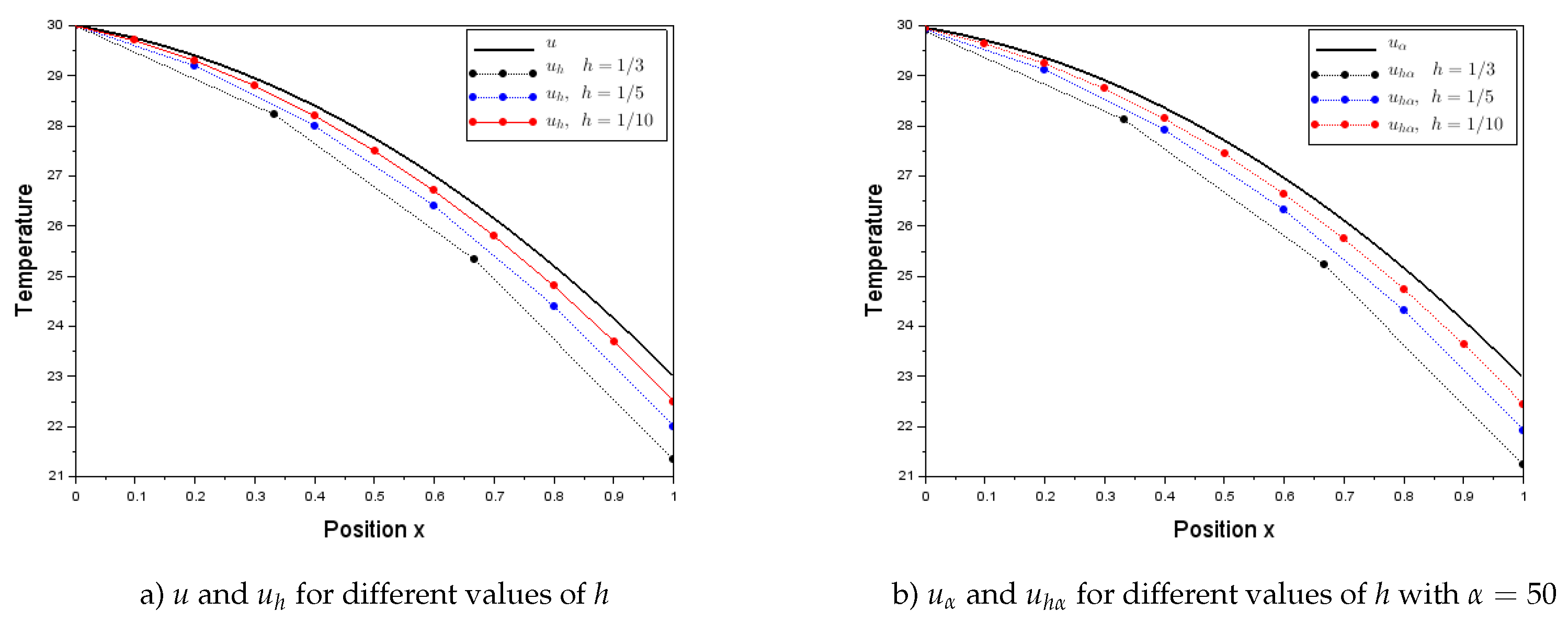
Figure 2.
Plot of u and against for different values of .
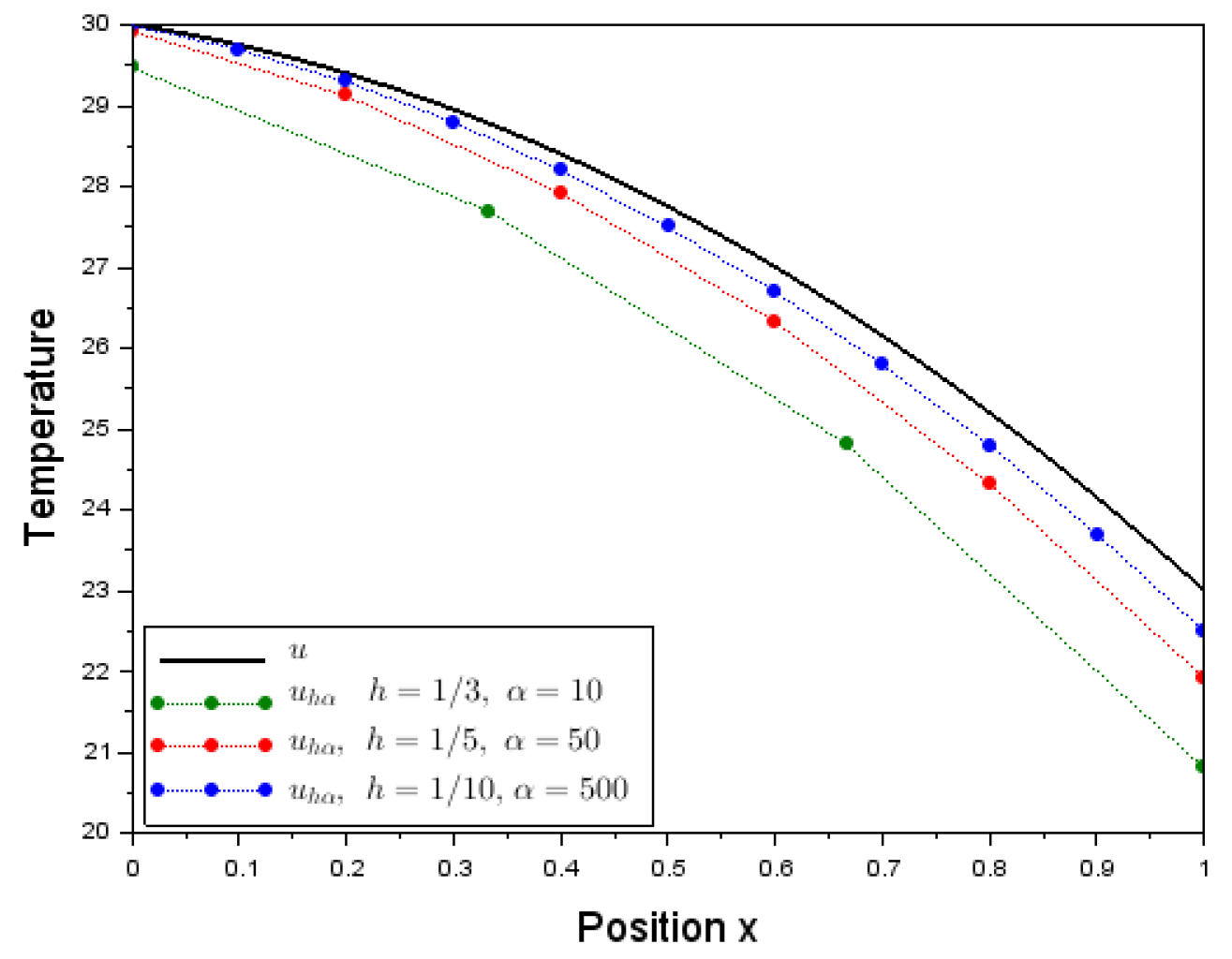
Figure 3.
Plot of , , and
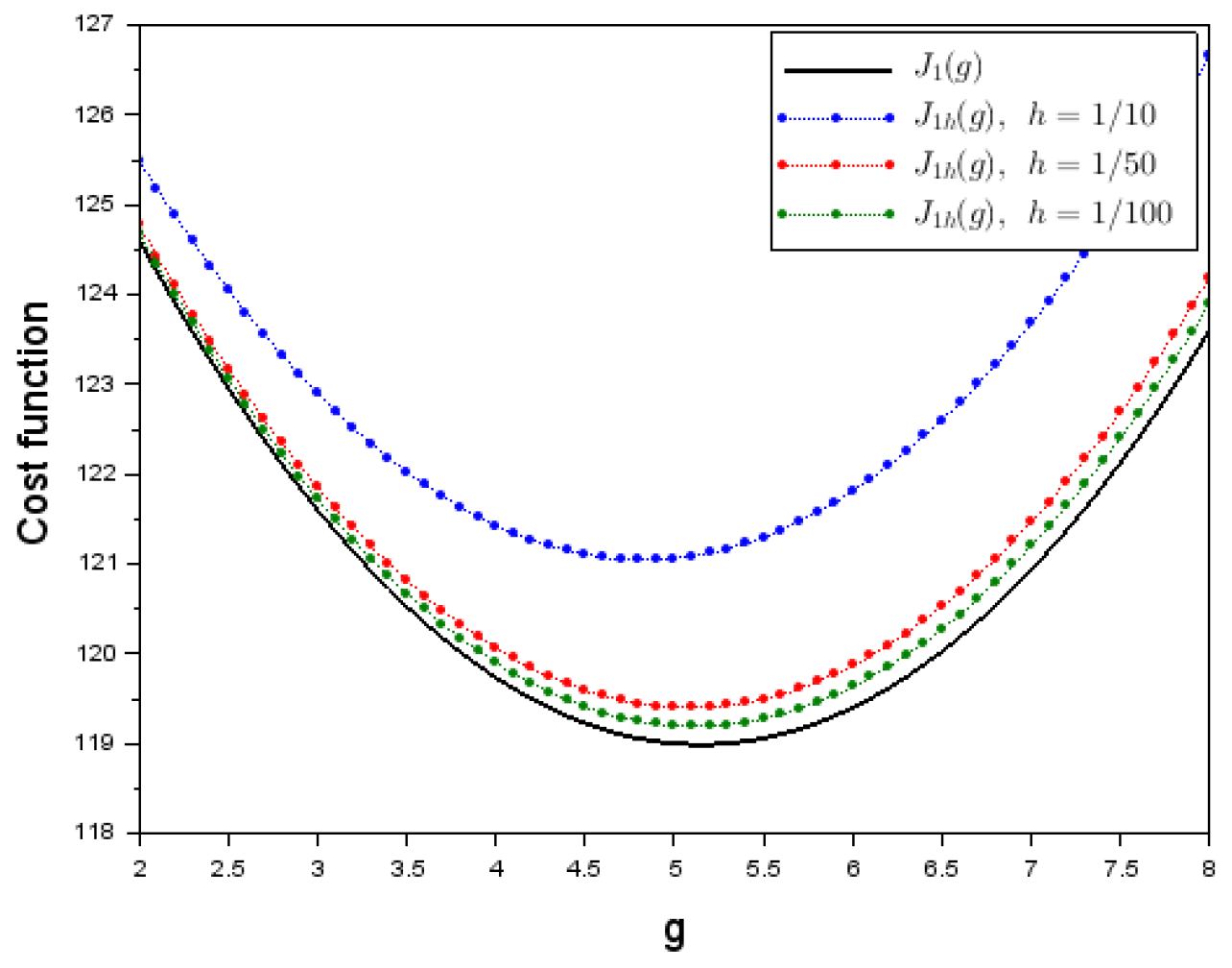
Figure 4.
Plot of , , and
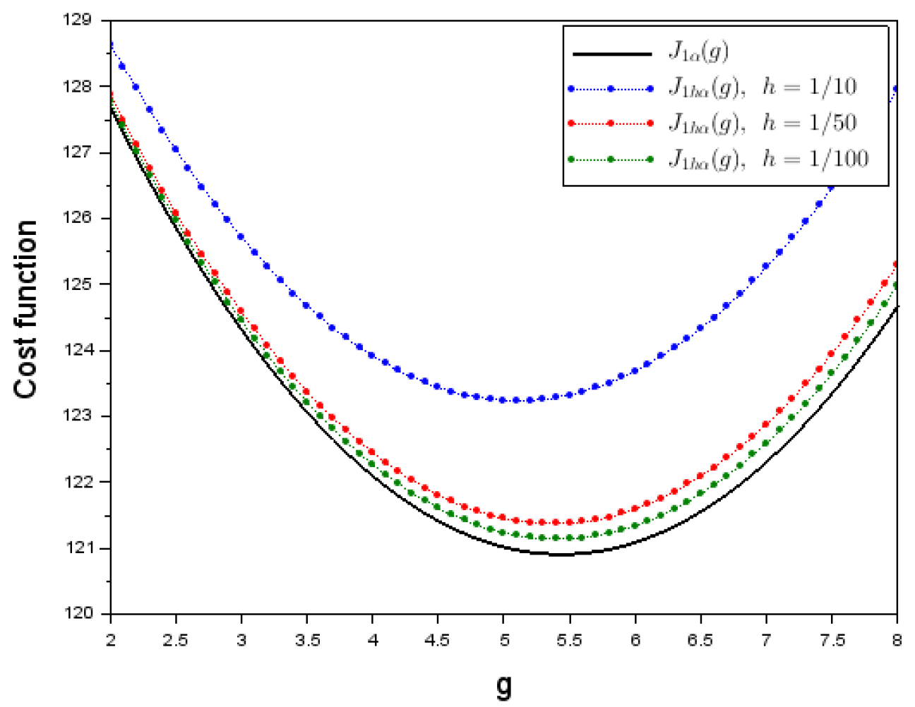
Figure 5.
Plot of , , and
Disclaimer/Publisher’s Note: The statements, opinions and data contained in all publications are solely those of the individual author(s) and contributor(s) and not of MDPI and/or the editor(s). MDPI and/or the editor(s) disclaim responsibility for any injury to people or property resulting from any ideas, methods, instructions or products referred to in the content. |
© 2025 by the authors. Licensee MDPI, Basel, Switzerland. This article is an open access article distributed under the terms and conditions of the Creative Commons Attribution (CC BY) license (http://creativecommons.org/licenses/by/4.0/).
Copyright: This open access article is published under a Creative Commons CC BY 4.0 license, which permit the free download, distribution, and reuse, provided that the author and preprint are cited in any reuse.


