
Submitted:
19 December 2025
Posted:
23 December 2025
You are already at the latest version
Abstract
Curtain deflector coating is a widely employed technique for producing thin, uniform films in numerous industrial applications. Near the corner region created by the interaction of the moving substrate and the falling liquid curtain, the flow dynamics are more complex. In this study, an analytical investigation is conducted for the steady, incompressible, and creeping flow of a Maxwell fluid, incorporating the Navier slip condition at the substrate. The governing nonlinear equations, derived from the conservation of mass and momentum, are solved using the Langlois recursive technique in combination with the inverse method, yielding an approximate third-order solutions for velocity, pressure, and stress fields. Finite and physically consistent stress distributions are produced by the slip condition that removes the singularity connected to the traditional no-slip boundary condition. The analysis demonstrates that substrate slip significantly reduces tangential stresses and enhances the stability of the coating flow. Residual error analysis is also performed to verify the accuracy and convergence of the analytical solutions. The results provide a deeper understanding of how slip effects can be utilized to improve coating uniformity and optimize the operational performance of curtain deflector coating systems.
Keywords:
maxwell fluid
; creeping flow
; curtain deflector coating
; slip condition
; langlois recursive approach
1. Introduction
Coating processes are widely employed in industry to deposit thin liquid or solid layers on moving substrates, with applications ranging from paper [1] and packaging to electronics [2,3], optics, and biomedical devices [4]. The primary goal is to achieve uniform films at high operating speeds while minimizing material waste and surface defects. A variety of techniques, such as blade coating [5], slot-die coating [6], and dip coating [7], have been developed, each with its own advantages and limitations. The curtain-deflector coating process presents several distinct advantages that enhance its suitability for producing continuous, defect-free coatings:
- Curtain coating can operate at very high web speeds (hundreds of m/min), making it suitable for mass production (e.g., photographic films, packaging, paper, and polymer coatings).
- Several liquid layers can be coated at once without intermixing, which is valuable for multilayer products (e.g., batteries, OLEDs, barrier films).
- The free-falling curtain naturally levels itself, producing a smooth, defect-free film with uniform thickness across large widths.
- Almost all of the liquid in the curtain is deposited on the substrate, making the process highly material-efficient.
- Since the curtain does not touch the substrate before deposition, it avoids streaks, scratches, or defects caused by doctor blades or rolls.
- Coating thickness can be controlled precisely by adjusting the flow rate and web speed.
Among these, curtain coating has attracted considerable attention due to its ability to produce highly uniform layers at industrially relevant speeds. In this method, a free-falling liquid curtain impinges on the substrate, allowing for smooth coverage across large widths. The introduction of a deflector in curtain coating provides an additional degree of control over the flow, redirecting and stabilizing the curtain before it reaches the substrate. In 1992, Kashiwabara et al. [8] provided experimental visualization of curtain coating flows, highlighting the formation and stability characteristics of liquid curtains under different operating conditions, which offered valuable qualitative insights into flow behavior and instabilities. Triantafillopoulos et al. [9] investigated operational issues in high-speed curtain coating of paper, identifying challenges such as curtain breakup and non-uniform coverage, while their subsequent study [10], examined curtain coating of lightweight coated papers, addressing process limitations and industrial applicability. In 2022, Schweizer [11] provided a comprehensive overview of the specific properties of curtain coating, emphasizing its unique advantages, operating limits, and comparison with other pre-metered coating methods. More recently, Zhan et al. [12] conducted numerical simulations of lacquer curtain formation, identifying flow regimes which advanced mechanistic understanding of curtain formation and stability.
The curtain deflector coating not only enhances uniformity and reduces instabilities but also creates a corner-like flow region between the curtain and the moving surface. The investigation of corner flows has attracted sustained attention due to their fundamental complexity and practical relevance in coating technologies. Strauss [13] presented one of the earliest systematic models for the flow established at a doctor blade in a coating apparatus, demonstrating how the blade edge induces strong gradients in stress and velocity that govern the quality of the applied film. This early work provided the foundation for subsequent studies on coating flows and motivated the need to understand fluid motion in confined geometries. Building upon viscous-flow theory, Cox [14] developed a rigorous analysis of liquid spreading on solid surfaces under creeping-flow conditions, establishing scaling laws and asymptotic behavior that remain central in the theoretical framework of wetting and coating. These Newtonian studies set the stage for the incorporation of complex rheology into corner-flow problems. In this direction, Bhatnagar et al. [15] investigated the flow of an Oldroyd-B fluid between intersecting planes and demonstrated that fluid elasticity not only alters the corner-flow structure but also mitigates singularities and redistributes stresses. Their results highlighted the importance of viscoelastic effects in coating flows, particularly when sharp corners or moving plates are involved. Complementary to this, Hills et al. [16] extended Taylor’s paint-scraper problem by introducing the concept of rotary honing, showing that rotating boundaries can generate closed streamline regions whose geometry directly influences coating efficiency.
Further progress was made by Siddiqui et al. [17], who analyzed the creeping motion of a second-grade fluid in a corner and concluded that non-Newtonian effects significantly modify the velocity field and stress distribution compared with Newtonian fluids, reinforcing the necessity of considering complex fluid behavior in real world processes. In parallel, Taylor et al. [18] examined viscoplastic corner eddies, producing fundamentally different corner dynamics than those observed in purely viscous or viscoelastic fluids. Together, these studies established that both elasticity and plasticity strongly influence the local flow topology in intersecting-plate geometries. Rehman et al. [19] analyzed Jaffrey–Hamel flow of an Oldroyd-B fluid between intersecting plates, showing that elasticity affects flow stability and symmetry, thereby providing deeper insights into the role of viscoelastic stresses in corner geometries. Finally, Yim et al. [20] offered a detailed analysis of low speed blade coating flows, showing that the flow can be decomposed into a flow offered by Taylor, thus linking the theoretical framework of corner flows with the operational parameters of industrial coating. Collectively, these contributions demonstrate that while early studies emphasized the singular structure of Newtonian corner flows, modern investigations reveal that viscoelasticity [21,22,23], viscoplasticity, and moving boundary effects profoundly reshape the flow field, making corner-flow analysis indispensable for advancing coating science and related applications.
In the context of corner flow problems, the Navier slip boundary condition holds considerable theoretical and practical significance. By incorporating slip, the singularities are alleviated, resulting in a more accurate description of fluid behavior near sharp edges or moving plates. Navier slip boundary condition was first proposed by Navier [24] in 1823, allows fluid velocity at a solid surface to have a finite slip proportional to the local shear stress, in contrast to the classical no-slip condition which assumes zero relative motion between the fluid and the wall. Dussan [25] provided one of the earliest systematic analyses of the moving contact line problem, showing that the classical no-slip boundary condition leads to a stress singularity and highlighting the role of slip boundary conditions as a resolution mechanism. This study demonstrated that introducing slip at the solid–liquid interface removes the mathematical inconsistency and offers a physically realistic description of contact-line motion. Later, Thompson et al. [26] used molecular dynamics simulations to investigate the dynamics of moving contact lines, confirming that slip naturally arises at molecular scales and directly affects both the velocity of the contact line and the dynamic contact angle. Their results established a strong microscopic basis for the slip boundary condition, thereby linking continuum fluid mechanics with molecular-level behavior. Together, these studies form the foundation of modern understanding of slip effects in moving contact line problems, motivating subsequent theoretical and computational developments. In a related direction, Koplik et al. [27] examined corner flows in the sliding plate problem using molecular dynamics simulations, focusing on the singular behavior of stresses near the corner. They demonstrated that slip at the wall naturally emerges at molecular scales and plays a critical role in regularizing the stress singularities. He et al. [28] carried out a numerical investigation of the classical driven cavity problem under the Navier slip boundary condition and showed that the presence of slip substantially modifies the flow structure by reducing corner singularities and smoothing velocity gradients near the walls. Their results highlighted the importance of slip length in controlling vortex strength and overall flow stability. These studies underline the fundamental role of slip effects in corner flow problems, showing how they alleviate stress concentrations and alter flow topology.

Table 1.
Novelty of the present work compared to previous study.
| Previous Study | 1975 Strauss [13] |
2003 Renardy [33] |
2011 Sprittles [34] |
Present study |
|---|---|---|---|---|
| Fluid model | Maxwell fluid | Maxwell fluid | Newtonian fluid | Maxwell fluid |
| Slip effects | ✕ | ✕ | ✓ | ✓ |
| Creeping flow | ✓ | ✓ | ✓ | ✓ |
| Normal and tangential stress analysis | ✕ | ✕ | ✕ | ✓ |
| Pressure distribution | ✓ | ✕ | ✓ | ✓ |
| Validation of the results | ✕ | ✓ | ✕ | ✓ |
This study solved the problem using Langlois recursive approach [29,30]. Langlois introduced a recursive approach to the theory of slow, steady viscoelastic flow, which provides a systematic way of generating successive approximations to the velocity, pressure and stress fields. This method is particularly valuable for handling the mathematical complexity of viscoelastic models by reducing higher-order constitutive relations into a recursive sequence of simpler problems. In his first work, Langlois [29] developed the recursive formulation, while in the follow-up study [30], he demonstrated its applicability to three fundamental hydrodynamic problems, Couette, Poiseuille and generalized Poiseuille flow. Building upon such analytical foundations, more recent contributions, such as Bakodah [31], have emphasized computational strategies for solving initial-boundary value problems with Neumann boundary conditions, showing how recursive or step-wise solution approaches can be effectively integrated with numerical schemes to address boundary-driven flow problems.
Table 2.
Comparison of Maxwell fluid with other fluid models.
| Model | Rheology | Suitability for Curtain Coating | Comment / Relevance |
|---|---|---|---|
| Newtonian | Constant viscosity | Poor |
|
| Power-law | Shear-thinning and thickening | Limited |
|
| Bingham / Herschel–Bulkley | Yield stress with shear-thinning | Limited | Captures yield-stress behavior, but less relevant for curtain coating, which involves continuous viscoelastic flow rather than solid-like behavior. |
| Jeffreys | Elasticity with Newtonian viscosity | Moderate | Describing both viscous and elastic effects, but involves more parameters and complicates analysis. |
| Oldroyd-B / PTT (Phan–Thien–Tanner) | Full viscoelastic model with relaxation and retardation times | Accurate but complex | Captures full elastic memory and stress evolution but introduces strong nonlinearity; challenging for analytical or semi-analytical treatment. |
| Maxwell | Single relaxation time; linear viscoelasticity | Best compromise |
|
The present study investigates the creeping flow of a Maxwell fluid in the corner region formed by the interaction between a falling liquid curtain and a moving substrate in a curtain deflector coating configuration. Despite considerable analytical and numerical research on curtain deflector coating and corner flows, limited attention has been given to Maxwell fluids under such conditions. This study suggests that the singularities typically arising near the contact line under classical no-slip conditions can be alleviated through the introduction of slip boundaries. However, the systematic application of advanced analytical techniques, such as the Langlois recursive approach combined with inverse methods, remains largely unexplored for creeping Maxwell flows in corner-dominated domains. To address these gaps, the present work develops an analytical model for the steady, incompressible flow of a Maxwell fluid incorporating a Navier slip boundary condition at the moving substrate. The governing nonlinear equations are solved using the Langlois recursive technique in conjunction with inverse methods to obtain closed-form expressions for velocity, pressure, and stress fields. Residual error analysis confirms the accuracy and convergence of the proposed solution. The addition of slip-induced regularization with viscoelastic effects constitutes a novel contribution, and producing finite and physically consistent stress distributions. The results offer valuable insights into the influence of slip on coating uniformity and provide a theoretical framework for optimizing curtain coating performance involving viscoelastic fluids.
2. Mathematical Modeling
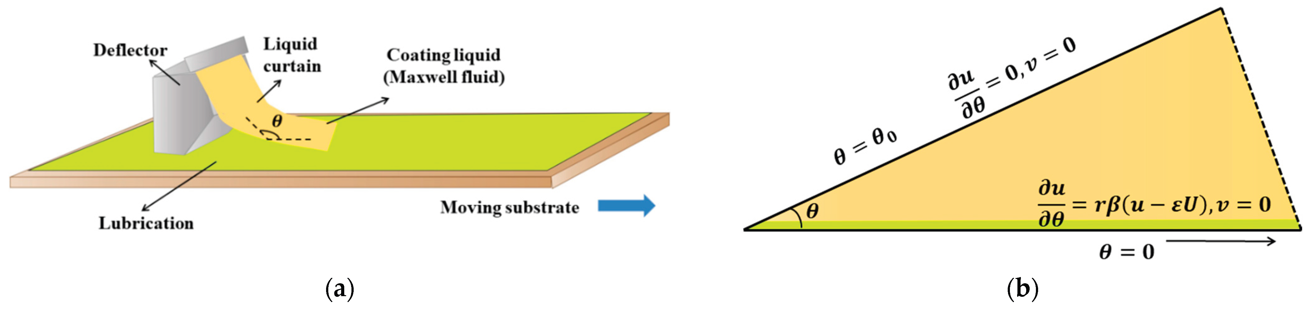
Consider a curtain–deflector with the Maxwell fluid as a coating liquid on a moving substrate. The substrate at translates with constant velocity, and slip effects are incorporated along the surface to capture realistic interfacial behavior. Due to the presence of the deflector, the liquid forms a curtain that impinges on the moving substrate at an angle , which generates a corner flow configuration.
Figure 1.
Geometry of the problem.
The following suppositions are also taken into account:
- The flow in the curtain coating process is assumed to be steady, laminar, and two-dimensional.
- The coating liquid is treated as a Maxwell fluid to capture the viscoelastic and relaxation characteristics typical for polymer-based coating materials.
- A polar coordinate system is adopted to describe the flow field and facilitate analysis in the corner region.
- The flow is creeping, implying that inertial effects are negligible compared with viscous and elastic forces.
- The flow develops in the corner region formed by a moving substrate and a falling liquid curtain, where the curtain makes an inclination angle θ with the substrate.
- The free surface of the falling curtain is assumed to be fixed and traction-free.
- A slip boundary condition is imposed along the moving substrate to represent the lubricated interaction between the coating film and the solid surface.
- Body forces due to gravity, are neglected in the present analysis.
The velocity field for the problem under consideration is:
The viscous flow around a corner can be studied by the following continuity and momentum equations:
where stands for constant density, shows the velocity vector, is the dynamic pressure, and S is symmetrical extra stress tensor of Maxwell fluid [33].
After using Eq. (1) in Eqs. (2)-(3), one can get the following expressions:
-component of momentum equation:
-component of momentum equation:
Where and are normal and tangential components of extra stress tensor of Maxwell fluid which satisfies the following relation:
where
where is the material derivative, represents the relaxation time, shows the dynamic viscosity, and is the first Rivlin-Ericksen tensor [32].
The lubricated moving substrate and fixed deflector satisfy the following boundary conditions:
and
Here, denotes the slip coefficient, is the radial distance corresponding to the substrate length, and represents the velocity of the moving substrate.
3. Methodology
To solve the problem the Langlois recursive technique [29,30] is used, originally introduced by William E. Langlois, which is designed to handle nonlinear governing equations by generating a hierarchy of linear or simplified problems that can be solved recursively. By using this technique, the velocity profile, pressure, and shear stress are expressed in terms of a series expansion and subsequently linearized with the aid of a small dimensionless parameter, which characterizes the order of non-linearity in the system.
Assume a series solution of the following form:
The velocity field considered for this problem is of the form:
The boundary conditions are:
The following dimensionless quantities are considered for this problem:
For analytical tractability, the analysis is restricted to terms up to third order in , while higher-order contributions are neglected due to the rapidly increasing complexity of the governing equations. Using Eqs. (12)-(19) into governing equations (6)-(11), one can get the first-order, second-order and third-order systems and their solutions.
3.1. First-Order Problem and Its Solution
The continuity and momentum equations for first-order problem are as follows:
Normal and tangential stress tensor for first order are expressed as:
Substituting Eq. (24), the continuity and momentum equations of first order (21)-(23) reduce to the following non-dimensional form:
where
And the boundary conditions are as follows:
Introducing the stream function which helps to reduce the number of dependent variables into a single variable.
Cross-differentiating Eq. (26) and (27) to eliminate pressure and then substituting Eq. (31) in the resulting equation and Eqs. (29)-(30), one gets the following expression:
with the following boundary conditions:
Assuming the solution of first-order stream function in the following form [32]
After using Eq. (35) in Eqs. (32)-(34) and then solving the differential equation, one can get the same result as mentioned in Ref. [32].
Substituting the above result of stream function into Eq. (31), one can get and , that are expressed as follows:
And the corresponding expression for the first-order pressure is given below:
where is constant.
3.2. Second-Order Problem and Its Solution
Continuity and momentum equation for second order takes the following form:
The stress tensor components of the second order are expressed as:
By substituting Eqs. (41)–(42) into Eqs. (39)–(40), the second-order form of the momentum equations is obtained as follows:
With the following boundary conditions:
To simplify the system by reducing the dependent variables into a single representation, the second-order stream function is introduced as follows:
By eliminating the pressure through cross-differentiation of Eqs. (43) and (44), and subsequently substituting Eq. (47), the following form is obtained:
With the following boundary conditions:
Assuming the solution of the second-order stream function in the following form:
By substituting the assumed second-order stream function solution (51) into Eqs. (48)–(50), the partial differential equation is reduced to an ordinary differential equation of the following form:
With the following boundary conditions:
The solution of Eq. (52-54) is calculated using the software Mathematica 12.0.
By substituting the previously obtained solution into Eq. (47), the second-order velocity components, and , are given as follows:
By substituting and from Eq. (55) into Eqs. (43)–(44), then integrating Eq. (43) with respect to , and subsequently differentiating the resulting expression with respect to after that a comparison with Eq. (44) yields the second-order pressure expression as follows:
3.3. Third-Order Problem and Its Solution
For the third-order problem, the continuity and momentum equations take the following form:
The non-dimensional form of the third-order stress tensor components is expressed as follows:
where are define in Appendix.
By substituting Eqs. (60)–(61) into Eqs. (58)–(59), the non-dimensional form of the momentum equations for the third-order problem is given as follows:
With the following boundary conditions:
To simplify the problem the third order stream function is introduced as below:
After cross-differentiating Eqs. (62) and (63), and employing Eq. (66), one can get the following:
With the following boundary conditions:
The solution for the third-order stream function is assumed in the following form:
Substituting Eq. (70) into Eqs. (67)–(69) yields the following ordinary differential equation:
Subject to the following boundary conditions:
Eqs. (71)-(73) are solved using software Mathematica 12.0.
After substituting the third-order stream function solution into Eq. (66), the expressions for the velocity components and takes the following form:
Applying the same procedure as in the second-order case, the pressure for the third order is given as follows:
It is important to note that the singularity arises at the sharp corner only in the pressure field. The classical singularity that typically appears in the velocity profile near the corner is effectively eliminated through the incorporation of slip effects, which provide a more realistic description of the flow behavior in such geometries.
Summarizing results up to the third order:
The normal stress is expressed as follows:
The tangential stress vanishes at the boundaries under slip conditions because the slip boundary allows relative motion between the fluid and the surface. As a result, the shear resistance at the wall vanishes, leading to zero tangential stress, this condition physically represents a surface where the fluid experiences no frictional drag.
The component of the total stress perpendicular to the curtain and the component parallel to the curtain are defined as follows:
3.4. Validation of Results
To verify the validity of the present analytical results, it is observed that as , the obtained solutions in Eqs. (76–81) reduce to the solution of creeping flow of a Newtonian fluid, which is consistent with the findings of Mahmood et al. [32]. Furthermore, to examine the accuracy of present formulation, a residual error analysis is performed by substituting the derived expressions of velocity, pressure, and stress given in Eqs. (76–81) into the governing Eqs. (5)-(6). This procedure yields the error functions and , which are presented in Table 03 and Table 04 for a range of positions within the flow domain. The reported values remain consistently small across the domain, indicating that the analytical approximations are in close agreement with the exact governing equations.
Table 3.
Error in -component of momentum equation.
| Residual error | |||||
|---|---|---|---|---|---|
|
|
|||||
Table 4.
Error in -component of momentum equation.
| Residual error | |||||
|---|---|---|---|---|---|
|
|
|||||
Table 5.
The numerical values of normal and tangential stress to the liquid curtain and substrate for different variations of .
Table 5.
The numerical values of normal and tangential stress to the liquid curtain and substrate for different variations of .
4. Graphs and Discussion
Figure 2 and Figure 3 illustrate the influence of the governing parameters on the velocity profile of the coating fluid. In the curtain coating process, the velocity distribution directly determines the uniformity and stability of the coated film. It is observed that increasing length of the moving substrate enhances the velocity field of the fluid. A longer substrate provides a greater contact area for the curtain to spread and stabilize before detachment, maintaining shear over a wider region. This promotes stronger transport of the coating liquid away from the corner, allowing the fluid to level more effectively and minimizing film thickness variations. Furthermore, Figure 2 and Figure 3 demonstrate the effect of the Navier slip parameter on the velocity profile. As increases, slip at the substrate surface becomes more significant, effectively lowering frictional resistance between the coating fluid and the substrate. This shows that the liquid layer experiences reduced drag, allowing smoother flow and better wetting of the substrate without excessive shear. Finally, an increase in the Weissenberg number is shown to amplify the velocity field. In the curtain coating context, a higher represents stronger elastic effects due to polymer chain stretching within the Maxwell fluid. This stored elastic energy assists in stabilizing the free-falling curtain and sustaining a continuous film, especially at high coating speeds. The 3D plots of the velocity field are given in Figure 4 to show this phenomenon.
Figure 5 illustrates the influence of the Navier slip parameter and the Weissenberg number on the normal stress distribution near the moving substrate in the curtain coating flow. In coating operations, the slip parameter represents the extent to which the coating liquid can slide over the substrate surface. A higher value of corresponds to smoother or more lubricated substrate conditions—such as those produced by pre-wetted, coated, or treated surfaces. As increases, the interfacial resistance between the liquid curtain and the moving substrate decreases, allowing the fluid to deform more freely. This reduced resistance shifts a greater portion of the strain from the substrate surface into the bulk of the coating film. Figure 5 reveals that an increase in the Weissenberg number which signifies stronger elastic effects, indicates that the fluid microstructure is unable to relax rapidly relative to the deformation rate imposed by the falling curtain and the moving substrate. As a result, the fluid elements experience greater elastic tension along the flow direction. This elastic stretching manifests as higher normal stresses near the coating corner region. Thus, understanding the interplay between slip and elasticity is crucial for optimizing coating speed, film uniformity, and substrate wetting in curtain coating of viscoelastic (Maxwell-type) fluids.
Figure 6 illustrates how the key parameters influence the pressure distribution in the curtain coating region. An increase in the Navier slip parameter reduces viscous resistance at the fluid–substrate interface. The coating liquid experiences less drag as it moves along the moving substrate. As a result, the liquid film accelerates more easily in the coating direction, which can promote smoother flow. However, to conserve mass and sustain the curtain flow, a higher pressure gradient is required to drive the fluid consistently along the coated surface. In practice, this corresponds to a stronger local pressure buildup in the coating bead, ensuring the curtain remains attached to the substrate and does not break away. Figure 6 shows how the substrate length affects the pressure distribution. A longer substrate allows the fluid to develop and redistribute velocity and stress more gradually. This corresponds to a longer contact region where the fluid can spread uniformly before being drawn downstream by the moving web. Consequently, the local pressure gradient required to sustain flow decreases with increasing substrate length, resulting in a more uniform and stable coating layer with reduced chances of flow instabilities or film thickness variations. Figure 6 also illustrates the effect of the Weissenberg number , which quantifies the ratio of elastic to viscous forces in the flow. As increases, the Maxwell fluid exhibits stronger elastic behavior due to a longer relaxation time. The elastic memory increases the normal stress within the fluid and resists flow deformation. To maintain a stable curtain and consistent flow rate, a larger driving force (or higher pressure gradient) becomes necessary. This results in an overall rise in pressure distribution within the coating bead. At very high values, excessive elastic stresses could lead to surface irregularities or curtain flutter, emphasizing the need to control viscoelastic properties of the coating fluid for smooth and defect-free film formation.
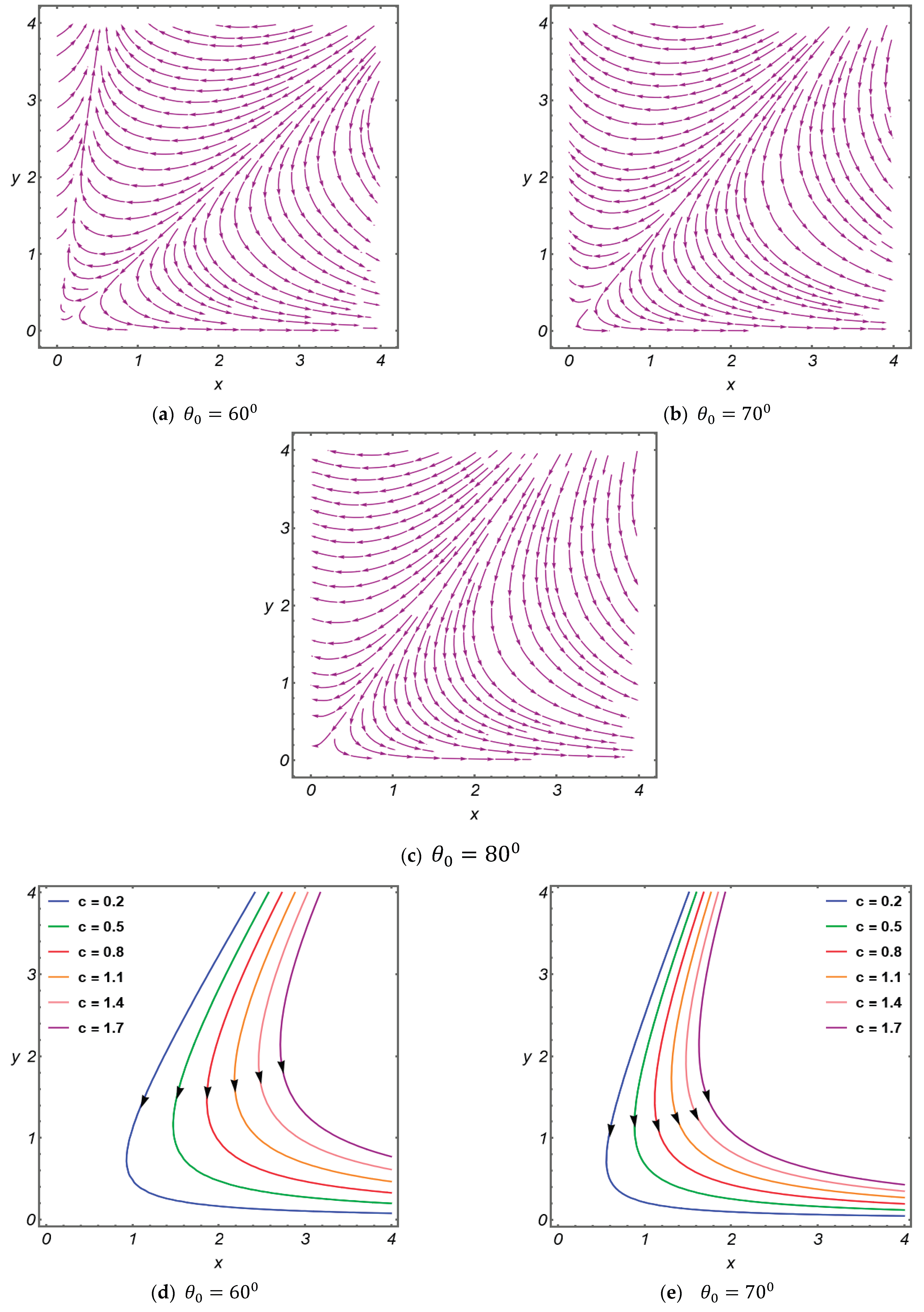
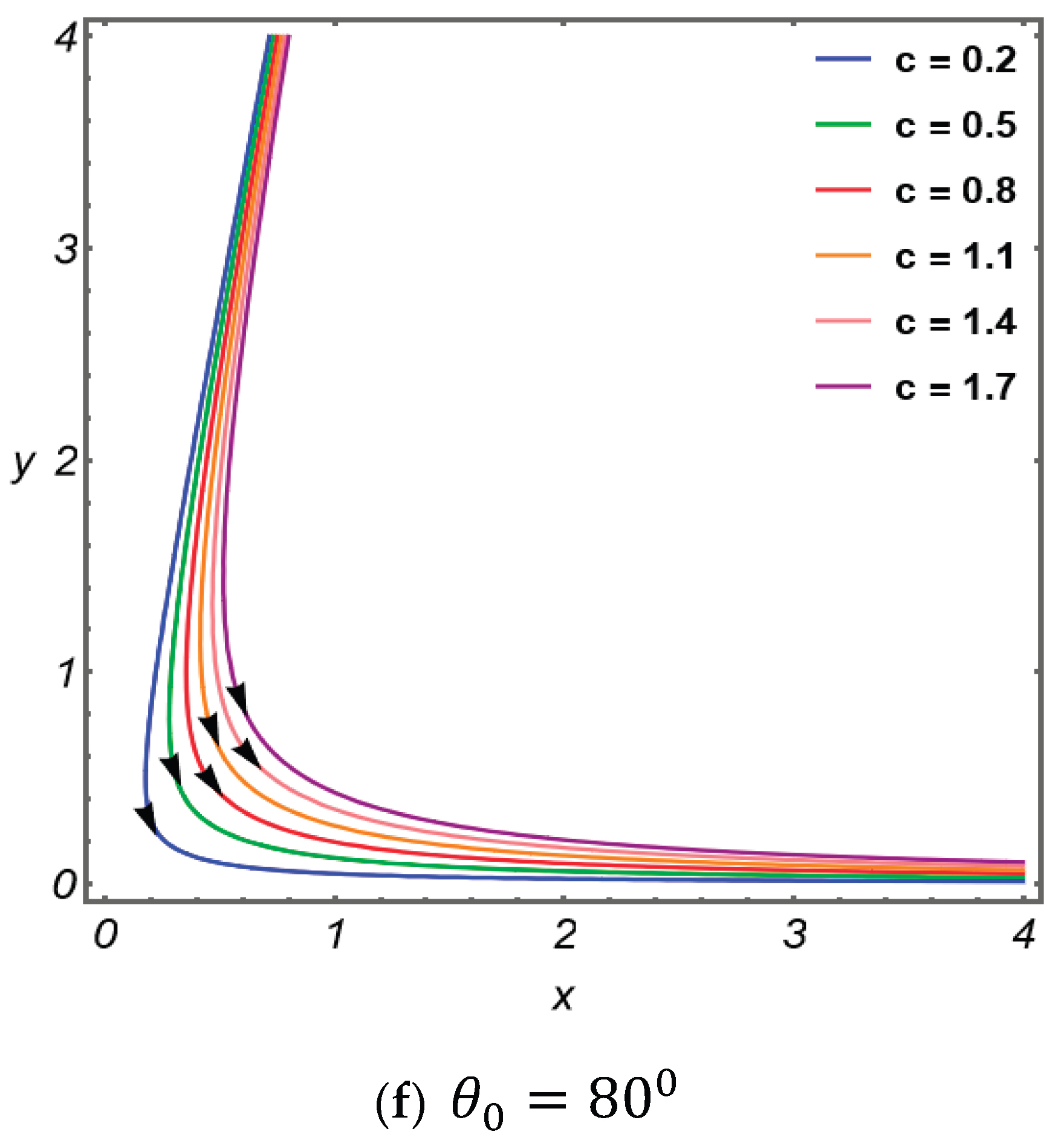
Figure 7 depicts the streamline patterns as affected by changes in the corresponding parameter related to the flow characteristics of a coating fluid. The introduction of a slip condition at the substrate allows limited tangential motion between the fluid and the substrate. The abrupt velocity discontinuity associated with the classical no-slip condition is eliminated. This relaxation of the boundary constraint prevents the buildup of excessive shear and effectively removes the singularity at the corner. As a result, the flow field becomes more physically realistic, exhibiting well-defined and regular streamline patterns that enhance coating uniformity and stability. Furthermore, as the curtain angle increases, this reduces local velocity gradients and stress buildup, promoting smoother streamline alignment and a more stable coating bead. This interaction defines the critical role of the slip condition and curtain angle in regularizing the flow dynamics at the corner.
5. Conclusions
In this study, a curtain coating with a deflector has been analyzed by considering Maxwell fluid as the coating liquid. The flow characteristics were examined under steady and creeping flow conditions near the corner formed between the liquid curtain and the moving substrate. To solve the governing equations, a combination of the Langlois recursive approach and the inverse method was employed, and the accuracy of the solution was verified through residual error analysis. The results demonstrate that the singularity at the corner can be effectively alleviated by incorporating a slip boundary condition, which provides a significant improvement in describing the flow behavior. Notably, under the slip condition, the tangential stress vanishes on both the substrate and the liquid curtain, whereas stress divergence occurs when the curtain and substrate are aligned either parallel or perpendicular to one another. These findings highlight the important role of slip in stabilizing the flow near sharp corners, leading to smoother streamline patterns and more controlled stress distributions. Such insights are valuable for optimizing curtain coating processes, offering potential benefits in improving coating uniformity and efficiency across a wide range of industrial applications.
Funding
There is no funding for this study, and authors declare that there is no conflict of interest.
Data Availability Statements
No datasets are generated or analyzed during the current study.
Nomenclature
| Symbol | Description | Unit |
| Length of the substrate | ||
| Angle between substrate and curtain | - | |
| Velocity field | ||
| Radial velocity component | ||
| Azimuthal velocity component | ||
| Dynamic pressure | ||
| Extra stress tensor of Maxwell fluid | ||
| Density | ||
| Relaxation time | ||
| Dynamic viscosity | ||
| Rivlin-Ericksen tensor | ||
| Slip coefficient | - | |
| Small perturbation parameter | - | |
| Reynolds number | - | |
| Weissenberg number | - | |
| Stream function | ||
| Stress perpendicular to the curtain | ||
| Stress parallel to the curtain | ||
| Total stress perpendicular to the curtain | ||
| Total stress parallel to the curtain |
Appendix
Continuity equation
Boundary conditions
First-order stress tensor form
Second-order stress tensor form
Third-order stress tensor form
References
- Rastogi, V. K., & Samyn, P. (2015). Bio-based coatings for paper applications. Coatings, 5(4), 887-930. [CrossRef]
- Licari, J. J. (2003). Coating materials for electronic applications: polymers, processing, reliability, testing.
- Akram, M., Arshad, N., & Braem, A. (2021). Fabrication of corrosion-resistant chitosan–gelatin–bioactive glass-ZnO/CeO2 hybrid coating on magnesium ZK60 alloy by AC-EPD. Journal of Taibah University for Science, 15(1), 312-320.
- Murata, H., Chang, B. J., Prucker, O., Dahm, M., & Rühe, J. (2004). Polymeric coatings for biomedical devices. Surface Science, 570(1-2), 111-118. [CrossRef]
- Chang, Y. H., Tseng, S. R., Chen, C. Y., Meng, H. F., Chen, E. C., Horng, S. F., & Hsu, C. S. (2009). Polymer solar cell by blade coating. Organic Electronics, 10(5), 741-746. [CrossRef]
- Patidar, R., Burkitt, D., Hooper, K., Richards, D., & Watson, T. (2020). Slot-die coating of perovskite solar cells: An overview. Materials Today Communications, 22, 100808. [CrossRef]
- Brinker, C. J. (2013). Dip coating. In Chemical solution deposition of functional oxide thin films (pp. 233-261). Vienna: Springer Vienna.
- Kashiwabara, Y., Ogawa, S., & Ozaki, K. (1992, September). Visualization of Curtain Coating Flows. In Flow Visualization VI: Proceedings of the Sixth International Symposium on Flow Visualization, October 5–9, 1992, Yokohama, Japan (pp. 211-214). Berlin, Heidelberg: Springer Berlin Heidelberg.
- Triantafillopoulos, N., Iiro, L., & Petri, P. (2001). Operational issues in high speed curtain coating of paper. Proc. TAPPI.
- Triantafillopoulos, N., Grön, J. O. H. A. N., Luostarinen, I., & Paloviita, P. (2004). Operational issues in high-speed curtain coating of paper, Part 2: Curtain coating of lightweight coated paper. Tappi journal, 3(12), 11-16.
- Schweizer, P. M. (2022). Specific Properties of Curtain Coating. In Premetered Coating Methods: Attractiveness and Limitations (pp. 625-667). Cham: Springer International Publishing.
- Zhan, J. M., Lin, K., Li, Y. H., & Hu, W. Q. (2024). Numerical simulation investigation of the mechanism of lacquer curtain formation in curtain coating. Engineering Applications of Computational Fluid Mechanics, 18(1), 2323127. [CrossRef]
- Strauss, K. (1975a). Modell der stromung, die sich am Rakelmesser einer Beschichtungsanlage Einstellt. Rheologica Acta, 14(12), 1058–1065. [CrossRef]
- Cox, R. G. (1986). The dynamics of the spreading of liquids on a solid surface. Part 1. Viscous flow. Journal of fluid mechanics, 168, 169-194. [CrossRef]
- Bhatnagar, R. K., Rajagopal, K. R., & Gupta, G. (1993). Flow of an Oldroyd-B fluid between intersecting planes. Journal of non-newtonian fluid mechanics, 46(1), 49-67. [CrossRef]
- Hills, C. P., & Moffatt, H. K. (2000). Rotary honing: a variant of the Taylor paint-scraper problem. Journal of Fluid Mechanics, 418, 119-135. [CrossRef]
- Siddiqui, A. M., Ahmad, A., & Ahmed, N. (2011). Creeping flow of a second grade fluid in a corner. Applied mathematical modelling, 35(2), 621-636. [CrossRef]
- Taylor-West, J. J., & Hogg, A. J. (2022). Viscoplastic corner eddies. Journal of Fluid Mechanics, 941, A64. [CrossRef]
- Rehman, S., Bouzgarrou, S., & Akermi, M. (2024). Jaffrey-Hamel flow features of Oldroyd-B model through intersecting plates. Journal of King Saud University-Science, 36(1), 102997. [CrossRef]
- Yim, H., & Nam, J. (2024). Analysis of low-speed blade coating flows. Journal of Fluid Mechanics, 978, A11. [CrossRef]
- Sudarmozhi, K., Iranian, D., & Alessa, N. (2024). Viscoelastic fluid flow on channel in porous medium with Soret and Dufour along with the effect of activation energy and suction and blowing. Journal of Taibah University for Science, 18(1), 2328869. [CrossRef]
- Hanif, H., Khan, A., Rijal Illias, M., & Shafie, S. (2024). Significance of Cu-Fe3O4 on fractional Maxwell fluid flow over a cone with Newtonian heating. Journal of Taibah University for Science, 18(1), 2285491.
- Karthikeyan, S., Ali, F., Loganathan, K., & Thamaraikannan, N. (2024). An implication of entropy generation in Maxwell fluid containing engine oil based ternary hybrid nanofluid over a riga plate. Journal of Taibah University for Science, 18(1), 2387925. [CrossRef]
- Navier, C. L. M. H. (1823). Mémoire sur les lois du mouvement des fluides. Mémoires de l’Académie Royale des Sciences de l’Institut de France, 6(1823), 389-440.
- Dussan V., E. B. (1976). The moving contact line: The slip boundary condition. Journal of Fluid Mechanics, 77(4), 665–684.
- Thompson, P. A., & Robbins, M. O. (1989). Simulations of contact-line motion: slip and the dynamic contact angle. Physical review letters, 63(7), 766. [CrossRef]
- Koplik, J., & Banavar, J. R. (1995). Corner flow in the sliding plate problem. Physics of Fluids, 7(12), 3118-3125. [CrossRef]
- He, Q., & Wang, X. P. (2009). Numerical study of the effect of Navier slip on the driven cavity flow. ZAMM-Journal of Applied Mathematics and Mechanics/Zeitschrift für Angewandte Mathematik und Mechanik: Applied Mathematics and Mechanics, 89(10), 857-868. [CrossRef]
- Langlois, W. E. (1963a). A recursive approach to the theory of slow, steady-state viscoelastic flow. Transactions of the Society of Rheology, 7(1), 75–99. [CrossRef]
- Langlois, W. E. (1964b). The recursive theory of slow viscoelastic flow applied to three basic problems of Hydrodynamics. Transactions of the Society of Rheology, 8(1), 33–60. [CrossRef]
- Bakodah, H. O., & Al-Zaid, N. A. (2018). Computational approaches to initial-boundary value problems with Neumann boundary conditions. Journal of Taibah University for Science, 12(5), 612-619. [CrossRef]
- Mahmood, A., & Siddiqui, A. M. (2017a). Two dimensional inertial flow of a viscous fluid in a corner. Applied Mathematical Sciences, 11, 407–424. [CrossRef]
- Renardy, M. (2003). Stress integration for the constitutive law of the upper convected Maxwell fluid near the corners in a driven cavity. Journal of non-newtonian fluid mechanics, 112(1), 77-84. [CrossRef]
- Sprittles, J. E., & Shikhmurzaev, Y. D. (2011). Viscous flow in domains with corners: Numerical artifacts, their origin and removal. Computer methods in applied mechanics and engineering, 200(9-12), 1087-1099. [CrossRef]
Figure 2.
Variation in radial velocity for
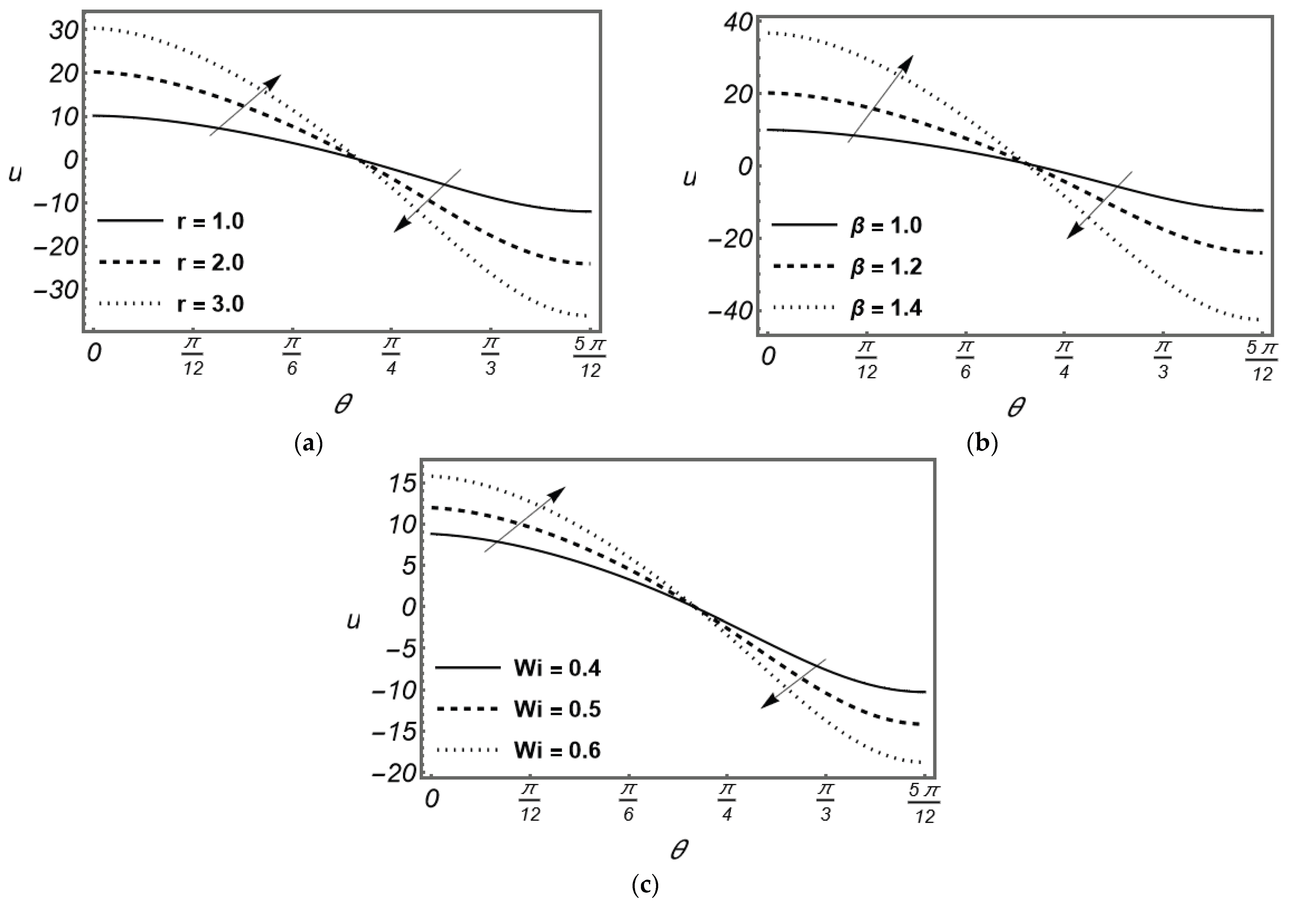
Figure 3.
Variation in azimuthal velocity for
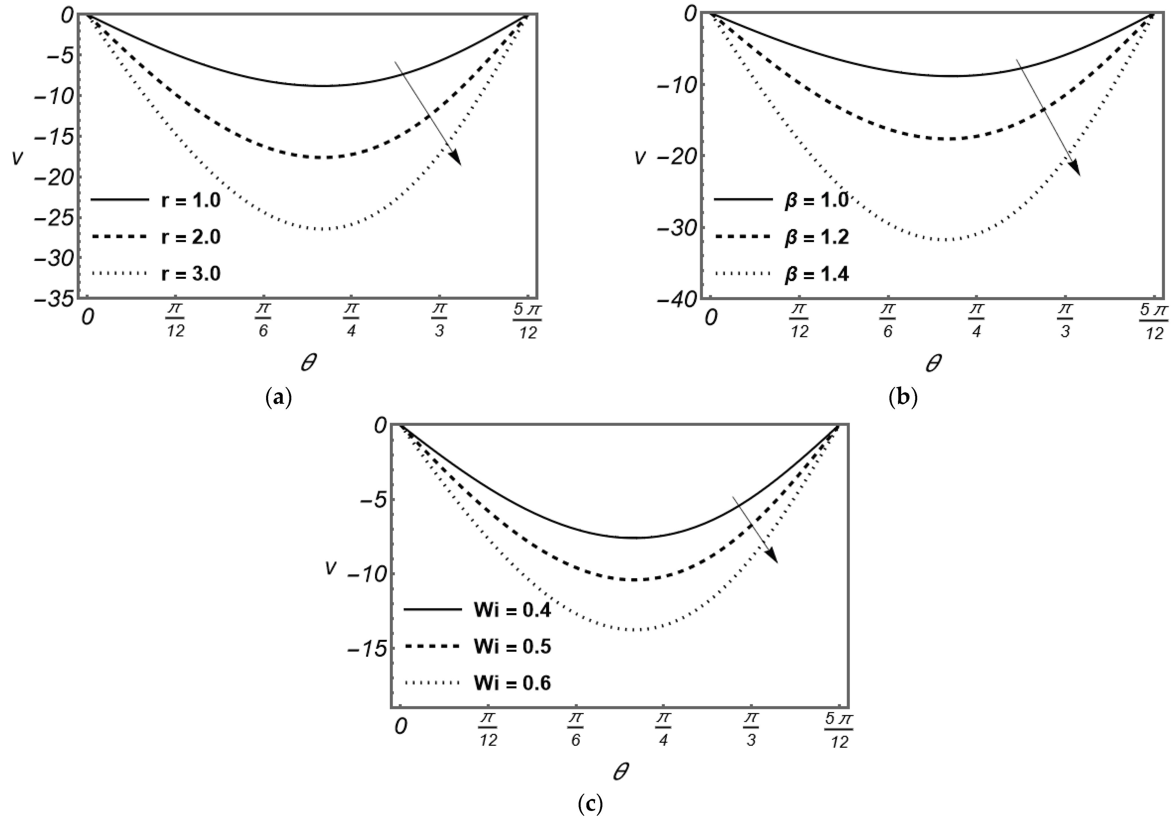
Figure 4.
3D view of curtain coating fluid flow in radial and azimuthal directions.
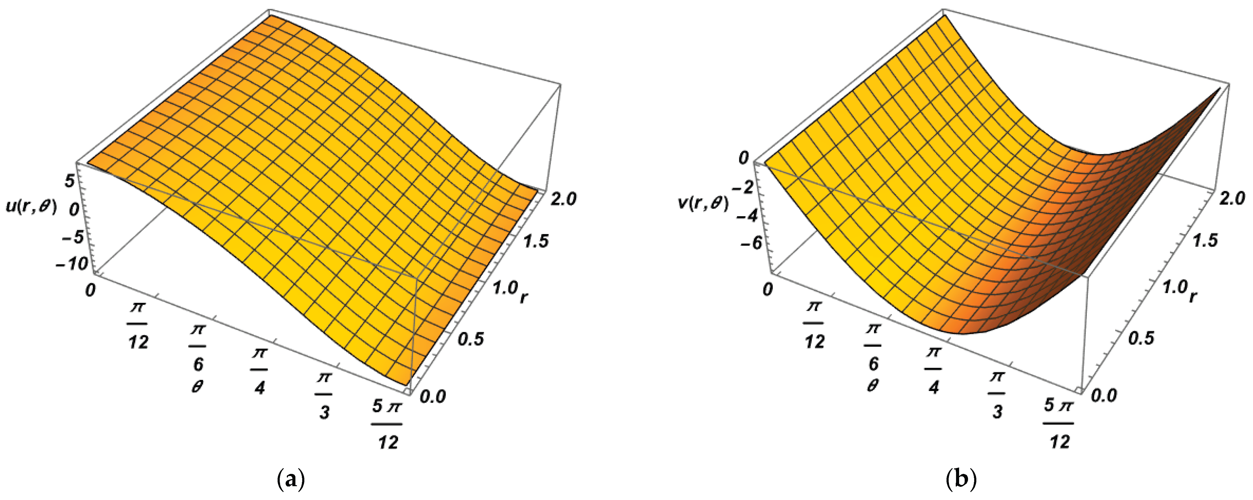
Figure 5.
Variation in normal stress for
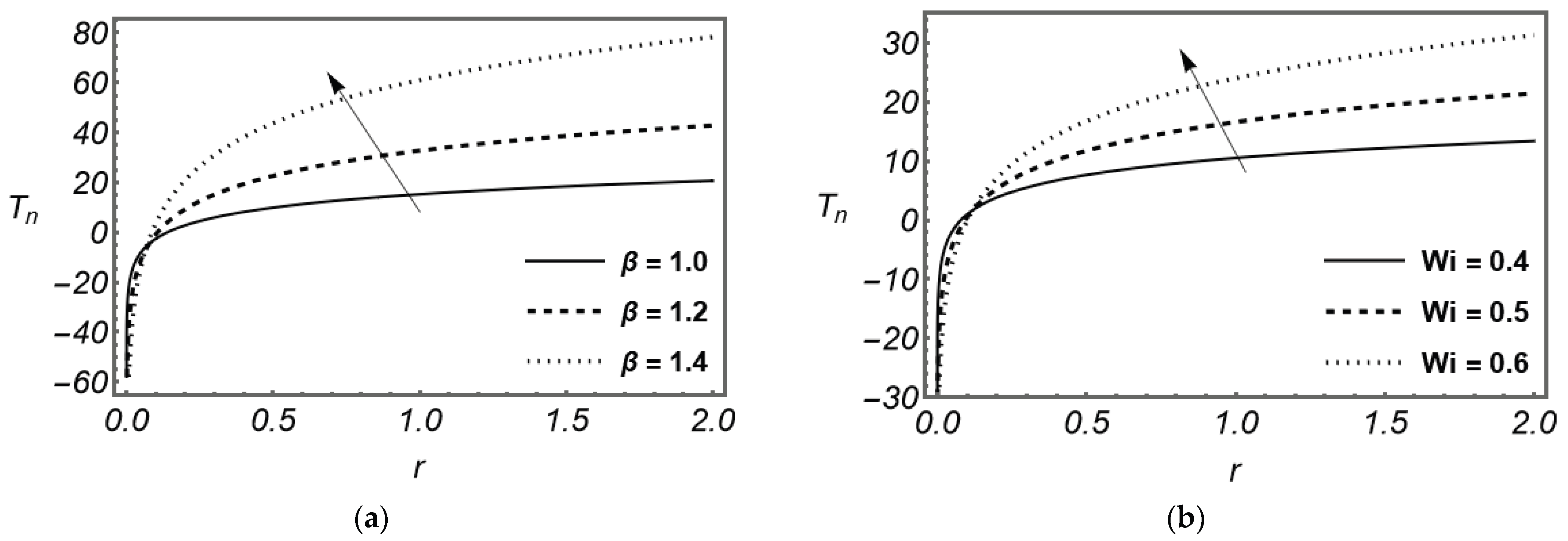
Figure 6.
Variation in pressure distribution for
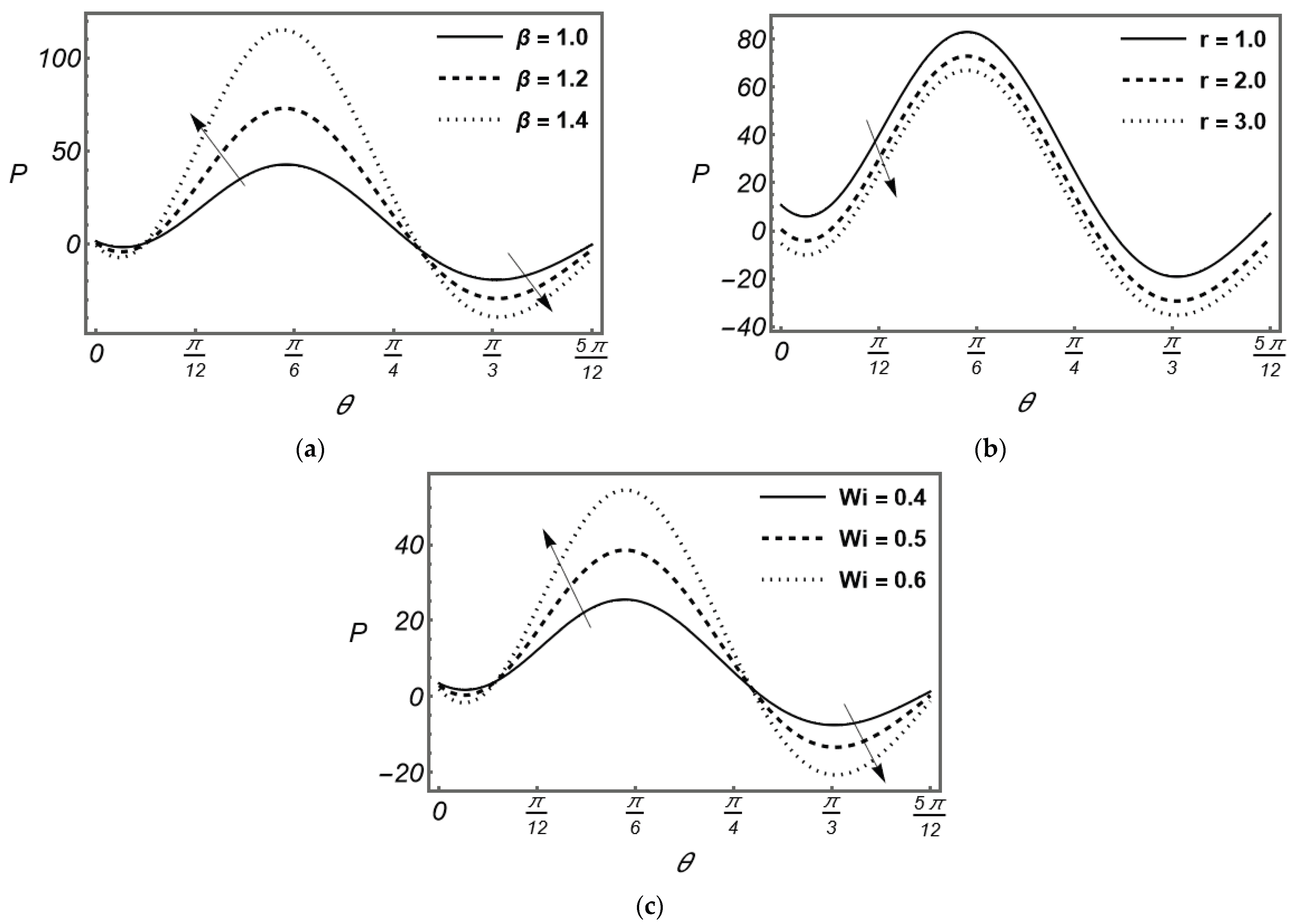
Figure 7.
Streamlines for different variations of liquid curtain angle
Disclaimer/Publisher’s Note: The statements, opinions and data contained in all publications are solely those of the individual author(s) and contributor(s) and not of MDPI and/or the editor(s). MDPI and/or the editor(s) disclaim responsibility for any injury to people or property resulting from any ideas, methods, instructions or products referred to in the content. |
© 2025 by the authors. Licensee MDPI, Basel, Switzerland. This article is an open access article distributed under the terms and conditions of the Creative Commons Attribution (CC BY) license (http://creativecommons.org/licenses/by/4.0/).
Copyright: This open access article is published under a Creative Commons CC BY 4.0 license, which permit the free download, distribution, and reuse, provided that the author and preprint are cited in any reuse.


