
Submitted:
18 December 2025
Posted:
22 December 2025
You are already at the latest version
Abstract
Background: Voice analysis combined with artificial intelligence (AI) is rapidly becoming a vital tool for disease diagnosis and monitoring. A key issue is the identification of vocal biomarkers, that are quantifiable features extracted from voice to assess a person’s health status or predict the likelihood of certain diseases. Currently, the biomarkers are extracted using pitch-asynchronized methods that need improvement. Methods: Based on the timbron theory of voice production, a pitch-synchronous method of vocal biomarker extraction is proposed and demonstrated on standard voice databases, especially the ARCTIC speech databases published by Carnegie Melon University. A complete set of formant parameters and timbre vectors for all US English monophthong vowels are presented. The timbre distances among all US English monophthong vowels are presented, showing the richness and accuracy of information contained in those biomarkers. Results: The methods are then applied on the voice recordings of the Saarbrücken voice database for voice diagnostics. Accurate and reproducible measurements of timbre vectors, jitter, shimmer, and spectral irregularity are generated, showing the usefulness to diagnostics-oriented voice signals. Conclusions: The biomarkers extracted using pitch-synchronous methods might have significant advantages for voice-based diagnostics over the traditional biomarkers. To quantify its effectiveness and accuracy, the pitch-synchronous methods should be tested on large-scale databases for diagnostics tasks to compare with the traditional biomarkers. Furthermore, the method of finding glottal closing instants from voice signals should be tested on voice databases for diagnostics tasks and live voice signals.
Keywords:
vocal biomarkers
; diagnostics
; timbre vector
; jitter
; shimmer
1. Introduction
Voice analysis combined with artificial intelligence (AI) is rapidly becoming a vital tool for disease diagnosis and monitoring [1,2,3,4,5,6,7]. For many decades, voice-based diagnostics has been applied in otorhinolaryngology to study voice disorders [1]. Because human voice is produced by a combination of several organs, voice-based diagnostics is shown to be applicable also to other medical disciplines [2]. For example, in neurology to diagnose and monitor dementia and Parkinson’s disease [3], in pulmonology for respiratory diseases [2,4], in oncology for early detection of many types of cancer including laryngeal cancer, throat cancer, oral cancer, and lung cancer [5]. Recently, it was also found that voice-based diagnostics can be effectively applied to detect and monitor heart failures [6].
Voice-based diagnostics have many benefits. It is non-invasive and can be more comfortable than traditional diagnostic procedures for patients. It enables early detection. It is easily accessible and with reduced costs. Especially, patients could monitor their health by submitting voice samples remotely to a healthcare provider, enabling ongoing evaluations and personalized care.
A key issue currently under intensive study is the identification of vocal biomarkers, that are quantifiable features extracted from voice signals to assess a person’s health status or predict the likelihood of certain diseases [2,8,9]. Currently, the traditional methods of feature extraction in speech technology [10,11] are used [6,13], including Mel-frequency cepstral coefficients (MFCCs) [14,15], linear frequency cepstral coefficient (LFCCs), the first two formants F1 and F2, and linear prediction coefficients (LPC) [30,31].
All the above biomarkers are extracted using pitch-asynchronous analysis methods. During the extraction process, a lot of vital information is lost. As we will show in this paper, based on a better understanding of voice production and pitch synchronous parameterization methods, better biomarkers can be extracted.
As presented in Subsection Physiology of Human Voice Production, human voice is generated a pitch period at a time, staring at each glottal closing instant (GCI) [18,19,20,21].The elementary sound wave triggered by each GCI, called a timbron, contains full information on the timbre. Continuous voice is generated by a superposition of a sequence of timbrons triggered by a series of glottal closing events. According to the timbron theory of voice production, the time difference between two adjacent GCIs defines the pitch period, and the sound waveform in each pitch period contains full information on the timbre.
To extract more information from voice signals, a pitch-synchronous analysis method is developed [18,19,20,21]. By using that method, pitch information and timbre information are cleanly separated. On average, the pitch period is 8 msec for men, and 4 msec for women. Therefore, for every 4 to 8 msec, a complete set of information on the timbre and pitch is obtained. The biomarkers extracted using a pitch-synchronous analysis method contain abundant, accurate, objective, and reproducible information from the voice signals that could improve the reliability of voice-based diagnostics.
The organization of the article is as follows.
In Section Methods, the history, the theory of voice production, and various methods for biomarker extraction are presented, examplified by the standard voice databases.
First, deficiencies of the traditional pitch-asynchronous analysis methods are analyzed. It was developed in the middle of the 20th century, when the computing power was low and computing languages were underdeveloped.As shown, a lot of vital information is lost during the extraction process.
Then, the timbron theory of voice production, a modern version of the transient theory, is presented as a logical consequence of the temporal correlation of the voice signals and the simultaneously acquired electroglottograph (EGG) signals. According to the timbron theory, the time difference between two adjacent glottal closing instants (GCIs) defines the pitch period, and the sound waveform in each individual pitch period contains full information on the timbre of the voice.
Further, a pitch-synchronous method of voice analysis is presented. By applying the pitch-synchronous analysis method to a standard US English speech corpus, the formant parameters of all US English monophthong vowels are measured. The correctness of the formant parameters is tested by voice synthesis, using a program appended to the article.
Because the format parameters have their limitations as biomarkers for voice-based diagnostics, the definition of timbre vectors together with the method of extraction, are presented. From a standard US English speech corpus, the timbre vectors for all monophthong vowels are presented. Especially, the timbre distances among all US English monophthongs are presented, showing the reliability and accuracy of the method.
In Section Results, using the pitch-synchronous analysis method, voice biomarkers including timbre vectors, jitter, shimmer, and spectral irregularity extracted from the Saarbrücken voice database are presented, showing their richness and accuracy. The Saarbrücken voice database were designed for voice-based diagnostics studies. The usefulness of the pitch-synchronous analysis method.
In Section VIII, the methods for detecting for this purpose is demonstrated. Because many voice recordings do not have simultaneously acquired EGG signals, the detection of GCIs from voice signals are presented. Based on the reference GCIs from the EGG, the accuracy of the methods of detecting GCIs from voice signals is analyzed.
In Section Discussions, the meanings of the methods and results are analysed. Recommendations for future research and applications are presented .
2. Methods
The evolution of digital voice analysis methods was closely related to the evolution of computing power. The methods of digital voice analysis were advanced and also limited by the available computing power at various stages of time. In the 1960s and 1970s, voice processing was implemented on mainframe computers with very low processing power. Accordingly, LPC, that requires low computing power, emerged at that time [30,31]. In the 1980s, PCs were born and evolved quickly. Fast Fourier transform (FFT) was applied to voice processing. MFCC was invented in 1980 [14], and then replaced LPC as the leading parametrization method for speech recognition.
The advantages of pitch-synchronous analysis for speech were recognized and studied in the 1970s and 1980s [16,17]. Nevertheless, it requires much higher processing power and did not become a mainstream. Pitch-asynchronous analysis methods prevailed.
2.1. Pitch-Asynchronous Analysis of Voice
The general procedure of pitch-asynchronous analysis is shown in Figure 1. Voice signal is typically blocked into frames with a duration of 25 msec and a shift of 10 msec, then multiplied with a window function, typically a Hamming window [10,11]. Because the windows are not aligned with pitch periods, pitch and timbre information are mixed. Even the voiced and unvoiced sections can be mixed, see Figure 1(A) and (B).
The use of frames of a fixed size is also mandated by the early fast Fourier transform (FFT). Traditionally, the size of source data for FFT must be a power of 2, typically 256 or 512. Because the windows are not aligned with the pitch boundaries, the output of FFT, the amplitude spectrum, is a mix of pitch periods and timbre properties, see Figure 2(A). The features are dominated by the overtones of the fundamental frequency, with an envelop associated with the formants.
The raw amplitude spectrum cannot be used as a biomarker. In the 1960s and 1970s, to extract usable features from the spectrum, the method of linear prediction coefficients (LPC) was introduced [30,31]. The short-time spectrum, showing in Figure 2(A), is approximated by an all-pole transfer function of order p. LPC is often applied to extract formants. Nevertheless, for each formant, the LPC method can only provide the frequency and the bandwidth. Level, an important parameter, is missing. Furthermore, the results of the frequencies using LPC method depend on an input parameter, the order p of the transfer function, see Figure 2. For example, with , the LPC analysis generates only one formant. With , three formants are shown. The one formant resulting from is not present. Therefore, that method is neither reproducible nor objective [10,31].
To extract timbre information from the short-time spectrum, in 1980, the method of Mel-frequency cepstral coefficients (MFCC) was invented [14] and gradually replaced LPC to become the most popular parameters for speech recognition [11]. To separate pitch information and timbre information, it bins the amplitude spectrum using a set of Mel-scaled triangular windows, to accommodate non-linear human perception of frequencies, as shown in Figure 3. Because the number of bins is limited, typically between 10 and 15, the frequency resolution is low.
By comparing with the rich information contained in voice signals available by using a pitch-synchronous analysis method, the MFCC has the following deficiencies, especially regarding voice-based diagnostics:
First, the quantity of feature vectors. Using the pitch-synchronous analysis method, a complete set of information can be obtained from each pitch period, which is roughly 8 msec for men and 4 msec for women. By using a fixed window size, typically 25 msec, the number of feature vectors is dramatically reduced.
Second, the quality of the feature vectors. To extract timbre information from a mix of pitch periods and formants, a binning procedure is taken, see Figure 3. The number of bins is typically 10 to 15. The frequency resolution is seriously limited. In contrast, by using a pitch-synchronous analysis method, the frequency resolution is virtually unlimited. It is practically determined by the quality of the original voice signals.
Third, objectiveness of the results. The window size and the window function significantly affects the results. Therefore, the MFCC coefficients are not objective.
Finally, reproducibility of the results. For example, by changing the starting point of the processing windows through a reduction or addition of silence changes the positions of the processing windows, and the MFCCs become different, which could affect the results of diagnostics.
By using a pitch-synchronous analysis method as shown in this paper, all those problems are resolved. Not only the quantity and quality of results are higher, but also the spectral coefficients are objective and reproducible. The results, for example the elements of timbre vectors, can be extracted from each pitch period. The processing frame boundaries are determined by the voice itself, not imposed manually.
The recent progress of computer hardware and programming languages enables the implementation of pitch-synchronous analysis methods. Coming to the 21st century, the evolution of computer power has been accelerated to be doubled in a few months. Owing to the growing computing power, Python programming language, although executes much slower than C++, became the most widely used programming language because of its readability and maintainability. Using the Numpy module of the Python language, FFT can be applied to an array of any size, not limited to power of 2. It greatly streamlines the implementation of pitch synchronous analysis methods.
2.2. Physiology of Voice Production
In order to define a better set of biomarkers and correlate the test results to a person’s health status and pathological conditions, a correct understanding of the physiology of voice production is necessary. Here we briefly outline a modern understanding of the physiology of human voice production, timbron theory [18,19,20,21].
The timbron theory of human voice production is a logical consequence of the temporal correlation of the voice signals and the simultaneously acquired electroglottograph (EGG) signals [18,19,20]. EGG was invented by French physiologist Philip Fabre in 1957 [25,26]. Since EGG is non-invasive and contains valuable information on the physiology of voice, it has become widely used [22,23,24]. A huge volume of speech recordings with simultaneously acquired EGG signals have been collected and published. The ARCTIC database, published by Carnegie Melon University, is a good example [27]. For the study of voice-based diagnostics, the Saarbrücken voice database, with 2250 voice recordings, available for free, was also collected with simultaneously acquired EGG signals [1,28].
The working principle of EGG is shown in Figure 4. Two electrodes are pressed against the right side and the left side of the neck, near the vocal folds. A high-frequency electrical signal, typically 200 kHz, is applied to one electrode, and an AC microammeter is placed on the other electrode, to measure the electrical conductance between the two electrodes. (a), while the glottis is open, the conductance is lower and then the ac current is lower. (b), while the glottis is closed, the conductance is higher and then the ac current is higher. The glottal closing instants (GCIs) can be determined accurately [22,23,24].
A ubiquitous experimental fact was observed in the temporal correlation between the voice signal and EGG signal [18,19,20], see Figure 5. Right after a GCI, (a), a strong impulse of negative perturbation pressure emerges. During the closed phase of glottis, (b), the voice signal is strong and decaying. In the glottal open phase, (c), the voice signal further decays and becomes much weaker. Immediately before a GCI, (d), there is a peak of positive perturbation pressure , which is a remnant of the glottal flow. The next GCI starts a new decaying acoustic wave, superposing on the tails of the previous decaying acoustic waves. The elementary decaying wave started at a GCI is determined by the geometry of the vocal tract, containing full information on the timbre, thus called a timbron. The pitch period is defined as the time interval of two adjacent GCIs. The observed waveform in each pitch period contains the starting portion of the timbron in the current pith period and the tails of the timbrons of previous pitch periods, therefore contains full information on the timbre of the voice around the time of that pitch period.
The acoustic process of generating an elementary sound wave characteristic to the vocal tract geometry is shown is shown in Figure 6. During the glottal open phase, step (0), air flows continuously from the trachea to the vocal tract. No sound is produced. At an abrupt glottal closing instant, step (1), the airflow is suddenly blocked. However, the airflow in the vocal tract keeps moving due to inertia. A negative-pressure wavefront is generated, which propagates with the speed of sound towards the lips, see (2). Then, the wavefront reflects from the lips and propagates towards the glottis, see (3) and (4). Because the glottis is closed, the wavefront is again reflected and propagates toward the lips. A complete formant cycle takes four back-and-forth propagations of the acoustic wave over the length of the vocal tract at the speed of sound. The time of a complete cycle is
here c is the speed of sound, 350 m/sec, and L is the length of the vocal tract. For male speakers, cm. One has msec, or a frequency of kHz. If the vocal tract is a lossless tube of uniform cross section, a square wave of 0.5 kHz is produced. The Fourier series of a square waves is
which can be observed as a series of formants centered at frequencies 0.5 kHz, 1.5 kHz, 2.5 kHz, and so on.
In general, loss of energy is unavoidable, and the shape of the vocal tract is different from a uniform tube. The waveform of an elementary sound wave triggered by a glottal closing with N formants is
Here the constants are the amplitude, related to the levels of the formants; are the bandwidth widths, and are the central frequencies of the formants. Note that before a glottal closing, , there is no acoustic signal. The glottis is open during the open phase. Nevertheless, the area of the glottis is much smaller than the mouth and the tissue surface of the vocal tract. The effect to the evolution of the decaying wave is minor. Therefore, the decaying wave continues until it disappears.
If there is a series of glottal closings with a constant time shift, or a constant pitch frequency, the next glottal closure starts a new decaying wave superposed on the tails of the previous decaying waves, see Figure 7. As shown, for different values of time shift, vowels with different pitch frequencies, for example, voice of = 125 Hz, 100 Hz, and 75 Hz can be produced.
The elementary wave triggered by a glottal closing is formed by the shape of the vocal tract, which contains full information on the instantaneous timbre. It is termed a timbron [18,19,20]. The fact that a timbron is zero before a glottal closing at has the following consequences, which can be proved with mathematical rigor [20].
First, the waveform in each individual pitch period is a superposition of the timbron in the current pitch period and the tails of the timbrons of the previous pitch periods. Therefore, the waveform in each pitch period contains full information on the timbre of the voice.
Second, according to a well-known mathematical theorem in the analysis of complex variables, the dispersion relation or the Kramers-Kronig relation, the phase spectrum is completely determined by the amplitude spectrum. Therefore, the amplitude spectrum contains full information on the entire waveform.
Third, in computing the Fourier transforms of the waveform in each pitch period, the starting point of waveform has no effect on the Fourier transform. It greatly simplifies the computation of the Fourier transform.
2.3. Pitch-Synchronous Analysis of Voice
As a demonstration of the pitch-synchronous method of extracting biomarkers from the voice signals, we use the ARCTIC database for speech science published by the Language Technologies Institute of Carnegie-Melon University [27]. Released in 2004, it became a standard corpus for speech science and technology. For each speaker, it has 1132 sentences carefully selected based on the requirement of phonetic balance from out-of-copyright texts of Project Gutenberg. The advantages of using this corpus as the first test are: The recordings were carefully collected under well-controlled conditions. It is phonetically labeled according to the ARPABET phonetic symbols [29]. It has simultaneously acquired EGG signals. In this paper, the voice of an US English speaker bdl is used. Note that some of the speech databases for voice-based diagnostics, such as the Saarbrücken voice database, also has simultaneously acquired EGG signals [1,28]. For voice recordings without EGG signals, GCIs can be detected from voice signals. We will discuss this issue in Section VII.
Figure 8 shows a small section of sentence a0329 by speaker bdl including the time derivative of EGG signal. The dEGG/dt curve shows sharp peaks at GCI points. Based on those GCI points, a series of segmentation points are generated. The voice signal is then segmented into pitch periods.
Because in general, right after segmentation, the value of the starting value A of the voice signal in a pitch period does not equal to the ending value C, an ends-matching procedure is executed, see Figure 9. For example, the original waveform in a pitch period is AC, an array wavin with 125 floating-point numbers. By taking 10 more points as CD, an array ext with 10 floating-point numbers is formed. Using the Python code,
for n in range(10):
x[n] = 0.1*float(n)
wavin[n] = wavin[n]*x[n]+ext[n]*(1-x[n])
the beginning section of the pitch period AB is replaced by the new section A’B. The ends are matched, and the curve is completely continuous, see Figure 9(b).
A key step is to take a digital Fourier transform on the waveform in each pitch period to generate spectra. In traditional FFT, the length of the data must be a power of 2, such as 256, 512, or 1024. Using the FFT modules in NumPy, a standard package of the Python programming language, the length of the array can be any integer. If the input sound wave is an array wavin with n points, the code
ampspec = np.abs(np.fft.rfft(wavin))
creates the amplitude spectrum of wavin with floating point numbers.
For most applications in voice-based diagnostics, vowel sounds are utilized. Here, the biomarkers for all monophthong vowels in US English are extracted. After the notation of ARPABET [29], there are 10 monophthongs, AA, AE, AH, AO AX, EH, IH, IY, UH, and UW. The diphthongs are represented as transitions from one monophthong to another one. Because the waveform in each individual pitch period contains full information on the timbre of the voice, for each monophthong, the waveform in a single pitch period suffices. Table 1 shows the source of each monophthong, including the sentence number, the time, and the word containing it.
The amplitude spectra of the 10 monophthong vowels are shown in Figure 10 and Figure 12 as blue dotted curves. As shown, those spectra contain rich information. Nevertheless, those amplitude spectra themselves are not appropriate to directly used as biomarkers. As usual, parametrization is necessary. Traditionally, the most used ones are formants and MFCC. In the following two sections, we show how to extract formant parameters and timbre vectors that are pitch-synchronous versions of MFCC.
3. Formant Parameters
2.1. Formant Parameters
Vowels were often characterized by a list of formants. Each formant is characterized by three parameters, central frequency , level , and bandwidth .
In the following, a method of extracting formant parameters from the amplitude spectra is described. If a timbron is described by Eq. 2, the amplitude of a complex Fourier transform of each term is
We now pay attention to the values of the amplitude spectrum at . The second term in the right-hand side is much smaller than the first term. Approximately,
In words, at each peak of the amplitude spectrum, where the frequency is , the amplitude is . As the first derivative of the curve is zero, the second derivative at the peak position is approximately
The second derivative can be estimated from the curve using the finite difference method by a small frequency increment, for example 50 Hz,
Under that approximation, the bandwidth is
After Eq. 5, the intensity constant is
Two examples are shown in Table 2. The central frequencies and the bandwidths are in unit of Hz. The amplitude parameter is in PCM unit. The sum of all intensity parameters is 32768. Therefore, while doing voice synthesis, the amplitude of the pcm is in a reasonable range. Intensity values for formants are very important. For example, by setting the amplitude of of AA to be 16000, and the amplitude value of to be small, it will sound like IY, rather than AA.
Figure 10 shows the amplitude spectra of all US English monophthong vowels, and the spectra recovered from the formants. First, we note that the pitch-synchronous amplitude spectra contain detailed information. Second, the amplitude spectra recovered from the formants represent essential information on the amplitude spectra.
To verify the correctness or the accuracy of the formant parameters, a Python program is designed to superpose the timbrons generated by those formant parameters, shown in Eq. 3, to become a melody sung with the vowel by a singer of various voices, including contrabass, bass, tenor, alto, soprano, or child.
Although the origin of the formant parameters is a tenor speaker, for other types of speakers, the formant parameters can be obtained by using a vocal-tract dimension factor, see Table 3. Because the formant frequency of a person is inversely proportional to the size of the vocal tract, the central frequency and the bandwidth are divided by the factor .
A list of all formant parameters of the monophthong vowels is included in an appendix. To test the accuracy of the formant parameters by singing synthesis, a Python program
melody.py
is included. For example, using the command
python3 melody.py Grieg AA 67 S 60
3. Timbre Vector and Timbre Distance
2.1. Timbre Vector and Timbre Distance
The formant parameters are intuitive and can be used for voice synthesis. However, they have limitations for voice-based diagnostics. The numbering of formants has some arbitrariness. For example, the strongest formant of vowel [AA] is at about 730 Hz [10]. It is typically identified as the first formant. But, there is often a weak formant at about 270 Hz. There is no objective criterion to label the 270 Hz peak or to label the 730 Hz peak as the first formant. Furthermore, the method represented by Eqs. 5 through 9 is based on an independent formant model, which requires that the frequency distance of adjacent formants is greater than the bandwidth of the formants. Otherwise, two formant peaks may merge, making them very difficult to separate from the amplitude spectrum.
To find a better mathematical representation of the amplitude spectrum, the experience of voice-based diagnostics is noticed: among all pitch-asynchronous biomarkers, MFCC is the best, due to the implementation of the Mel scale [1,2,3,4,5,6]. The pitch-synchronous equivalent of MFCC is timbre vectors [20], by implementing the Mel scale using a standard mathematical tool of Laguerre functions [32].
2.2. Laguerre Functions
2.1.1. Laguerre Functions
A Laguerre function is the product of a weighing function with a Laguerre polynomial [32]. The first two Laguerre polynomials are
For , the Laguerre polynomials are defined by the recurrence relation [32]
Using a simple program, all Laguerre polynomials can be generated. A Laguerre function is the product of a weighing function and a Laguerre polynomial
They are orthonormal on the interval ,
The waveforms are shown in Figure 11. As shown, the behavior of the Laguerre functions closely resembles the behavior of the Mel scale [32]. The first few Laguerre functions describe the gross features of the low-frequency amplitude spectrum. The later Laguerre functions represent the high-frequency spectrum and refine the low-frequency spectrum. Overall, the frequency resolution in the range of 0 kHz to 1 kHz is high, and the resolution at higher frequencies gradually becomes lower.
2.1.2. Definition of Timbre Vector
The amplitude spectrum of a timbron can be approximated by a sum of N such Laguerre functions [20],
where the coefficients are
The scaling factor is a constant with a dimension of time, having a convenient unit of msec, chosen to optimize accuracy. The final results are insensitive to its value. For example, ranging from = 0.1 msec to = 0.3 msec, the results are virtually identical.
The coefficients form a vector, denoted as . The norm of the vector
represents the overall amplitude. The normalized Laguerre spectral coefficients, constitute a timbre vector
represents the spectral distribution of the pitch period, characterizing the timbre of that pitch period independent of pitch frequency and intensity. Obviously, the timbre vector is normalized:
In this paper, we use 32 Laguerre functions, to generate a 32-componant timbre vector. To unify data format and save storage space, each component of the timbre vector is multiply by 32768 and expressed as type numpy.int16 in Python. Because the pcm is also in numpy.int16, it is sufficiently accurate. Each timbre vector is then stored as 64 bytes of binary data. To compute timbre distance, as shown later, the stored values are first divided by 32768 to become floating-point numbers.
Figure 12 shows the amplitude spectra of all US English monophthongs and the spectra recovered from the timbre vectors. As shown, the agreement is excellent, showing the accuracy of the timbre-vector representation. As biomarkers, the timbre vectors have significant advantages over the formants. The numbering of formants is somewhat arbitrary. It is difficult to compare two sets of formants. The timbre vectors are generated automatically and objectively. Especially, there is a well-defined and well-behaved timbre distance between two timbre vectors from two pitch periods, as shown below.
2.1.3. Timbre Distance
A critical parameter in any parametrical representation of speech signal is the distortion measure, or simply distance. Because the timbre vectors are independent of pitch frequency and intensity, the distances defined here can be justly characterized as timbre distance between a pair of timbre vectors and .
where and are the components of the two timbre vectors, or the arrays of the normalized Laguerre spectral coefficients and , see Eq. 15 through 18. The accurate definition of timbre distance makes the timbre vector a prime choice for voice-based diagnostics.
A list of timbre distances among the 10 US English monophthong vowels is shown in Table 4. As expected, the values differ significantly for various pairs. The maximum timbre distance is 2, when all components of one vowel is non-zero, the correspondent timbre vector elements of another vowel is zero. As shown in Table 4, many timbre distances of pairs of vowels are greater than 1, indicating a significant spectral difference. The timbre distance between [IH] and [AX] is small. This is expected because those two phones are often interchangeable.
We have shown how to do voice synthesis using formants. Using timbre vectors, voice synthesis can also be implemented, and it is often even better than using formants. Details are shown in Chapter 7 of the reference book [20]. Using dispersion relations, the phase spectrum can be recovered from the amplitude spectrum. Using reverse FFT from Numpy, individual timbrons can be recovered. By superposing the timbrons according to a music score, singing voice can be synthesized [38,39].
3. Results
The methods have been applied to the Saarbrücken database, published by Saarland university in 2007, designed for diagnostic studies especially for the contrast between the normal voices and various types of pathological voices [28]. It consists of voice signals with simultaneously acquired EGG signals from 2225 speakers. Here we report an initial study of the signals of a normal voice, to show the abundance, reproducibility, and accuracy of the timbre vector as a biomarker.
3.1. Timbre Vectors from the Saarbrücken Database
Figure 13 shows graphical representations of three recordings in the Saarbrücken database, the vowels [a], [i], and [u] spoken by speaker 88. There are simultaneously acquired EGG signals. The time derivative of the EGG signal is shown in Figure 13(a). As shown, in each pitch period, there is a prominent peak, especially a sharp rising edge, signifies the beginning of a pitch period. As the sampling rate of the Saarbrücken database is 50 kHz, the beginning of a pitch period, or the GCI, can be determined to an accuracy of 0.02 msec. See the red dashes in Figure 13(b). In Figure 13(b), it is also shown that the waveforms in individual pitch periods are similar. By taking a Fourier transform of the waveform in each pitch period, the amplitude spectrum is obtained, as shown in Figure 13(c) as a dotted blue curve. For each pitch period, a timbre vector can be obtained. Then, the amplitude spectrum is recovered using Eq. 15. Shown by solid red curves, the recovered spectrum matches nicely with the original amplitude spectrum. As shown in Table 5 and Figure 13, the number of timbre vectors are 308, 277, and 172 for the vowels [a], [i], and [u], respectively. The number is much greater than the number of MFCCs, each one shows a much higher resolution than MFCC, and are completely reproducible.
The details of the study, in the Appendix, show the advantage of using timbre vectors versus formant parameters. The Python source code and the original data are included in the Appendix. As shown, in many cases, such as the vowel [a], the formant curves are significantly overlapped such that some peaks do not show up. The timbre vectors, although less intuitive than the formants, are more reliable and reproducible.
3.2. Jitter, Shimmer, and Spectral Irregularity
Jitter and shimmer are often used as biomarkers for voice disorders [33,34], and now also as biomarkers for other medical conditions, see a recent review [35]. Jitter means the frequency variation of the sound wave over adjacent pitch periods, and shimmer means the amplitude variation of the sound wave over adjacent pitch periods. Within the framework of the source-filter theory of voice production, there are no valid definitions of jitter and shimmer. Both jitter and shimmer are described as perturbations to the source of voice, which originally should have a constant pitch [34,35].
Usually, jitter and shimmer are measured by asking the patient to produce several vowels in a steady frequency and volume, then by looking on the voice waveforms using a dedicated software, such as SEARP citepJitter2013. or a free software such as PRAAT [36]. For certain vowels, in each pitch period, there is a unique sharp peak at the same time instant in each pitch period, see Figure 14(a). The time between two adjacent peaks is defined as the pitch period. The intensity is determined by the value of the peak. However, for some vowels such as [IY] and [EH], the waveform has multiple peaks, and the determination of the pitch period is compromised, see Figure 14(b). On the other hand, for other vowels, for example [OH] and [UW], there are no sharp peaks in the voice waveform, and the determination of the pitch period is also compromised, see Figure 14(c).
According to the timbron theory of voice production, human voice is generated a pitch period at a time. Each glottal closing triggers an decaying elementary acoustic wave called a timbron. Because the timing and the intensity of each timbron is independent, jitter and shimmer are intrinsic to the nature of human voice. Based on the timbron theory, the methods of measuring jitter and shimmer can be precisely defined in terms of the pitch-synchronous analysis method, see Figure 14(a), (b), and (c), based on the GCI in each pitch period. If simultaneously acquired EGG signals are available, such as the Saarbrücken voice database [28], GCIs can be accurately determined. Such measurements are objective and reproducible, important for diagnostics.
Following the timbron theory of voice production, the pitch period is the time difference between two adjacent GCIs, a series of pitch periods are found for each vowel. Denoting them as , where N is the number of pitch periods, following the usual definition of relative jitter [34,35], we have
Usually it is expressed as percentages. For the three recordings from speaker 88 in the Saarbrücken voice database [28], the number of jitter are shown in Table 5.
For the shimmer, following the standard definition of decibels, the energy level in each pitch period can be defined by adding the energy of each pcm point,
where is the m-th pcm in period i having a total number of pcm points. The unit of pcm will cancel out. The definition is independent of the polarity of pcm. The shimmer in terms of decibel is
For the three vowel recordings from speaker 88 in the Saarbrücken voice database [28], the numbers of shimmer are shown in Table 5.
There is yet another parameter that can be precisely defined, the spectral irregularity. The timbre in each pitch period can be precisely represented by its timbre vector, which is normalized with a well-defined timbre distance, see Eqs. 19 and 20. The timbre distance between two adjacent pitch periods
is always non-negative. Therefore, a simple average can be applied. The average spectral irregularity of a voice recording with N pitch periods can be defined as
3.3. Detecting GCIs from Voice Signals
For voice recordings with simultaneous acquired EGG signals, for example the CMU ARCTIC database [27] and the Saarbrücken database [28], GCIs can be easily identified from the EGG signals to implement pitch synchronous analysis. Many voice recordings do not have simultaneous acquired EGG signals. Nevertheless, because of the importance of pitch synchronous speech signal processing, since the 1970s, methods to detect GCIs from voice signals have been developed. A recent review evaluated and compared five most successful methods to decent GCIs from voice signals based on the analysis of voice waveforms [37]. By applying those methods to the CMU ARCTIC database and taking the EGG based GCI as the reference, it is found that many methods can produce more than 80% of GCIs within 0.25 msec from the reference GCIs [37]. It is often sufficiently accurate for voice-based diagnostics.
Here we present a simple and useful method to detect GCIs from voice signals [20]. For the voice records in the Saarbrücken voice database [28] presented here, the program as a concise Python code is included in the Appendix. It uses an asymmetric window function to find the peak amplitudes in each pitch period to generate the GCIs,
where N is the width of the asymmetric window, see Figure 15. Near the ends, and , the asymmetric window function approaches zero as the third power of the distance to the ends, which generates very little disturbance.
To find segmentation points, the derivative of the voice signal is convoluted with the asymmetric window to generate a profile function, see Figure 16. The peaks of the profile function point to GCIs. By applying this method on the three Saarbrücken voice recordings, the GCIs from the voice signals are found to be consistent with those from the EGG signals. The Python code and all data sets are included in the Appendix.
The width of the asymmetric window N is an input parameter. However, the results are insensitive to the value of N. For example, for the vowels [a] and [u] by speaker 88 of the Saarbrücken database, using N between 130 and 330 (3.1 msec to 6.6 msec), the GCIs produced are virtually identical. Therefore, to execute that program, it suffices to have an estimate of the average pitch of the voice recording to an accuracy of -30% to +50%. As a rule of thumb, using the average pitch period, 8 msec for men and 4 msec for women as the width, the GCIs produced are reliable. By using the GCI points detected from voice signals as segmentation points, the values of jitter, shimmer, and spectral irregularity are reevaluated. The results are similar, see Table 6. By comparing with Table 5, one finds that the values of jitter are smaller. The values of shimmer and spectral irregularity are virtually identical to those obtained from the EGG data. Therefore, the GCIs detected from voice signals are basically reliable for extracting pitch-synchronous biomarkers.
For the ARCTIC databases, a detailed study was conducted in 2014, as reported in Section 5.4 in Reference [20]. Table 7 shows a summary of the results for a male speaker bdl and a female speaker slt. As shown in Table 7, for both bdl and slt, the GCIs detected from EGG but missing in the GCIs detected from the voice signal is only about 1%. In other words, about 99% of the GCIs from the EGG signals are recovered from the voice signals using the asymmetric window method. On the other hand, the number of GCIs detected from the voice signals are more than 10% greater than the number of GCIs derived from EGG signals. The origin of the difference is shown in Figure 17.
A detailed inspection finds that most of the extra GCIs are legitimate pitch marks, see Figure 17, which is part of sentence b0413, spoken by female speaker slt, an isolated word “or”. The vertical lines pointing up are pitch marks generated from the voice signals. In section A, the vocal folds start to vibrate and produce several periods of acoustic wave, but there are no complete glottal closures. In Section B, the vibration of vocal folds is strong enough to generate complete glottal closures. In Section C, the vibration of vocal folds is weakened, and incomplete closures appear again. A few more periods of acoustic wave are produced. The asymmetric window method relies on the low-frequency components of the voice signal, which works for complete glottal closures as well as incomplete glottal closures. For the purpose of determining the voiced sections versus unvoiced sections and to segment the voiced signals, those extra GCIs detected from the voice signals using the asymmetric windows method are useful rather than superfluous.
Furthermore, because the method of asymmetric windows only relies on the lowest Fourier components of the pitch frequency, and the noise signals are primarily in the high-frequecy range, that method might be fairly immune to noise.
4. Discussions
By applying the pitch-synchronous analysis method to standard general-purpose voice databases, including the ARCTIC voice database from Carnegie-Melon University, and the Saarbrücken database for voice-based diagnostics, many biomarkers are extracted. As shown, the quality and the quantity of the biomarkers extracted from those databases exceed the quality and the quantity of the biomarkers using the traditional pitch-asynchronous methods. There are three categories.
First, the formant parameters. Using the traditional pitch-asynchronous analysis methods, the intensity or level parameters of formants cannot be determined. The values of the central frequencies depend on an input parameter, the order of the all-pole transfer function, making the values of central frequencies subjective and nonreproducible. Using pitch-synchronous analysis methods, for each formant, three parameters, the central frequency, the bandwidth, and the intensity or level can be accurately extracted from the waveform in each pitch period. And the values are independent of any input parameters. As evidence of the accuracy of those parameters, creative voice synthesis can be generated from the formant parameters, including classical vocal music masterpieces [38,39].
Second, timbre spectra and timbre vectors. Using the pitch-asynchronous method, the typical representation of the timbre spectra is MFCC. Nevertheless, the frequency resolution of the MFCC coefficients are limited by the choice of binning intervals, and the results depend on the choice of window size and window function. The pitch-synchronous analysis method provides a more accurate version of MFCC, the timbre vectors based on a standard mathematical method, the Laguerre functions. The definition is simple and straightforward. The accuracy and reproducibility of the timbre vectors are far superior than MFCC. The number of timbre vectors, one from each pitch period, is greater than the number of MFCCs, which is one per process window.
Third, for the measurement of jitter and shimmer, the pitch-synchronous analysis method provides the values according to the basic definitions. Furthermore, a spectral irregularity can be defined and measured. And the available numbers of original data points are greater than those using the method of fixed windows.
Both ARCTIC and Saarbrücken voice databases have simultaneous acquired EGG signals, facilitating pitch-synchronous study. For databases without simultaneous acquired EGG signals, GCIs must be extracted from the voice signals. A method of detecting glottal closing instants using an asymmetric window has been applied to the entire ARCTIC database, and the GCIs thus detected are comparable from the point of view of extracting biomarkers. For the Saarbrücken databases, because of the relatively short and uniform nature the voice signals, the implementation of the GCI detection program is fairly straightforward. The asymmetric-window based method of GCI extraction should be tested on large-scale diagnostics orientated databases to verify and to improve.
Those new methods have not been tested on large-scale voice databases for diagnostics tasks. It will depend on the participation of the medical community to implement it on real-life data to reach definitive conclusions. Because the timbron theory and the pitch-synchronous analysis method only existed for several years, there are not many reference books and review articles to explain them. To make the concepts and methods easy to understand, this article contains a tutorial with simplified mathematics.
Availability of Supplemental Materials
In An appendix, two complete collections of the program and datasets are provided. The first part, ARCTIC, contains many original voice recordings and GCI text files from that database, with all source code written in Python, to generate formant parameters and timbre vectors and for demonstrating voice synthesis and computing timbre distances. The Python program for demonstrating voice synthesis based on the formant parameters is also included. The second part, Saarbrücken, contains representative original voice and EGG data, and all necessary programs written in Python, to generate timbre vectors as well as values of jitter, shimmer, and spectral irregularity. Programs to extract GCI from EGG data and voice data written in Pythion are also included. The programs for extracting GCIs from the ARCTIC databases and the intermediate datasets are too big to be included in an appendix, which can be requested through Columbia Technology Ventures.
Funding
This research received no external funding.
Data Availability Statement
All data used here is publicly available.
Acknowledgments
The formant parameters determination algorithm in this article was developed during an intensive international coorporation [21]. The author sincerely thanks Mathias Aaen of Nottingham University Hospitals, United Kingdom and Complete Vocal Insitute, Copenhagen, Denmark; Ivan Mihaljevic of Supersonic Songbird, Zagreb, Croatia; Aaron M. Johnson of NYU Grossman School of Medicine, New York; and Ian Howell of Emboded Music Lab, Ann Arber, Minnesota for providing high-quality voice recordings and inspiring discussions.
Conflicts of Interest
The author declares no conflicts of interest.
Abbreviations
The following abbreviations are used in this manuscript:
- AI
- Artificial intelligence
- MFCC
- Mel-frequency cepstral coefficients
- LFCC
- Linear frequency cepstral coefficients
- LPC
- Linear prediction coefficients
- EGG
- Electroglottograph
- GCI
- Glottal closing instant
- FFT
- Fast Fourier transform
References
- Sankaran, A; Kumar, L. Advances in Automated Voice Pathology Detection: A Comprehensive Review of Speech Signal Analysis Techniques. IEEE Access 2024, 12, 181127. [Google Scholar] [CrossRef]
- Fagherazzi, G; Fischer, A; Ismael, M; Despotovic, V. Voice for Health: The Use of Vocal Biomarkers from Research to Clinical Practice, Biomarkers from Research to Clinical Practice. Digital Biomarkers 2021, 5, 78–88. [Google Scholar] [CrossRef] [PubMed]
- De Silva, U; Madanian, S; Olsen, S; Templeton, J; Poellabauer, C. Clinical Decision Support Using Speech Signal Analysis: Systematic Scoping Review of Neurological Disorders. Journal of Medical Internet Research 2025, 27, e63004. [Google Scholar] [CrossRef]
- Kapetanidis, P; Kalioras, F; Tsakonas, C; Tzamalis, P; Kontogianannis, G; Stavropoulus, T. Respiratory Diseases Disgnosis Using Audio Analysis and Artificial Intelligence: A Systematic Review. Sensors 2024, 24, 1173. [Google Scholar] [CrossRef] [PubMed]
- Ankishan, H; Ulucanlar, H; Akturk, I; Kavak, K; Bagci, U; Yenigun, B. Early Stage Lung Cancer detection from Speech Sounds in Natural Environments. [CrossRef]
- Bauser, M; Kraus, F; Koehler, F; Rak, K; Pryss, R; Weiss, C; et al. Voice Assessment and Vocal Biomarkers in Heart Failure: A Systematic Review; Heart Failure: Circulation, August 2025. [Google Scholar]
- Mekyska, J; Janousova, E; Gomez-Vilda, P; Smekal, Z; Rektorova, I; Eliasova, I; Mrackova, M. Robust and Complex Approach of Pathological Speech Signal Analysis. Neurocomputing 2015, 167, 94–111. [Google Scholar] [CrossRef]
- Baghai-Ravary, L; Beet, SW. Automatic Speech Signal Analysis for Clinical Diagnosis and Assessment of Speech Disorders; Springer, 2013. [Google Scholar]
- Wszolek, W. Selected Methods of Pathological Speech Signal Analysis. Archives in Acoustics 2006, 31, 413–130. [Google Scholar]
- Rabiner, LR; Schafer, RW. Digital Processing of Speech Signals; Prentice-Hall: Englewood Cliff, New Jersey, 1978. [Google Scholar]
- Rabiner, LR; Juang, BH. Fundamentals of Speech Recognition; Prentice-Hall, New Jersey, 1993. [Google Scholar]
- Fant G, Acoustic Theory of Speech Production; (Molton & Co., The Hagues, The Netherlands 1960).
- Daly, I; Hajaiej, Z; Gharsallah, A. Physiology of Speech/Voice Production. Journal of Pharmaceutical Research International 2018, 23, 1–7. [Google Scholar] [CrossRef]
- Davis, SB; Mermelstein, P. Comparison of Parametric Representations for Monosyllabic Word Recognition in Continuous Spoken Sentences. IEEE Transaction on ASSP 1980, 28, 357–366. [Google Scholar] [CrossRef]
- Nagraj, P; Jhawar, G; Mahalakshmi, KL. Cepstral Analysis of American Vowel Phonemes (A Study on Feature Extraction and Comparison). IEEE WISPNET Conference, 2016. [Google Scholar]
- Hess, WJ. A pitch-synchronous digital feature extraction system for phonemic recognition of speech. IEEE Transactions on ASSP 1976, ASSP-24, 14–25. [Google Scholar] [CrossRef]
- Medan, Y; Yair, E. Pitch synchronous spectral analysis scheme for voiced speech. IEEE Trans. ASSP 1989, 37, 1321–1328. [Google Scholar] [CrossRef]
- Svec, JG; Schutte, HK; Chen, CJ; Titze, IR. Intgegrative insights into the myoelastic theory and acoustics of phonation. Scientific tribute to Donald G. Miller". Journal of Voice 2023, 37, 305–313. [Google Scholar] [CrossRef] [PubMed]
- Chen, CJ; Miller, DG. Pitch-Synchronous Analysis of Human Voice. Journal of Voice 2019, 34, 494–502. [Google Scholar] [CrossRef]
- Chen, CJ. Elements of Human Voice; World Scientific Publishing, 2016. [Google Scholar]
- Aaen, M; Mihaljevic, I; Johnson, AM; Howell, I; Chen, CJ. A Pitch-Synchronous Study of Formants. Journal of Voice 2025. [Google Scholar] [CrossRef]
- Baken, RJ. Electroglottography. Journal of Voice 1992, 6, 98–110. [Google Scholar] [CrossRef]
- Herbst, CT. Electroglottography - An Update. Journal of Voice 2020, 34, 503–526. [Google Scholar] [CrossRef]
- Miller, DG. Resonance in Singing; Inside View Press, 2008. [Google Scholar]
- Fabre, P. Un procédé électrique percutané d’inscription de l’acclement glottique au cours de la phonetion: glottographie de haute fréquence. premiers résultats. Bulletin de l’Académie nationale de médecine 1957, 141, 66–69. [Google Scholar]
- Fabre, P. La glottographie électrique en haute fréquence, particuralités de l’appareillage. Comptes Rendus, Sociéte de Biologie 1959, 153, 1361–1364. [Google Scholar]
- Kominek, J; Black, A. CMU ARCTIC Databases for Speech Synthesis. CMU-LTI-03-177; CMU Language Technologies Institute, Tech report. 2003. [Google Scholar]
- Woldert-Jokisz, B. Saarbrucken voice database. 2007. [Google Scholar]
- See Wikipedia entry of ARPABET. In some publications, the r-colored phones ER and AXR are also listed as monophthongs. In CMU pronunciation dictionaries, there is no AXR.
- Atal, BS; Hanauer, LS. Speech Analysis and Synthesis by Linear Prediction of the Speech Wave. J. Acoust. Soc. Am. 1971, 50, 637–655. [Google Scholar] [CrossRef]
- Markel, JD; Gray, AH. Linear Prediction of Speech; Springer Verlag: New York, 1976. [Google Scholar]
- Arfken, G. Mathematical Methods for Physicists.; Academic Press: New York, 1966. [Google Scholar]
- Brockmann, M; Drinnan, MJ; Storck, C; Carding, PN. Reliable Jitter and Shimmer Measurements in Voice Clinics: The Relevance of Vowel, Gender, Vocal Intensity, and Fundamental Frequency Effects in a Typical Clinical Task. Journal of Voice 2011, 25(1), 44–53. [Google Scholar] [CrossRef] [PubMed]
- Teixeria, JP; Oliveria, C; Lopes, C. Vocal Acoustic Analysis – Jitter, Shimmer and HNR Parameters. Procedia Technology 2013, 9, 1112–122. [Google Scholar] [CrossRef]
- Jurca, L; Viragu, C. Jitter and Shimmer Parameters in the Identification of Vocal Tract Pathologies. Current State of Research. Springer Proceedings in Physics, Acoustics and Vibration of Mechanical Structures – AVMS-2023, 2025; pp. pp 155–164 Springer. [Google Scholar]
- Boersma, P; van Heuven, V. Speak and unSpeak with Praat. Glot International 2001, 5, 341–347. [Google Scholar]
- Drugman, T; Thomas, M; Gudnason, J; Naylor, P; Dutoit, T. Detection of Glottal Closure Instants from Speech Signals: a Quantitative Review. arXiv arXiv:2001.00473v1. [CrossRef]
- https://vimeo.com/1096282984, Puccini’s Humming Chorus in Madama Butterfly, synthesized using a formant model.
- https://vimeo.com/1096287185, Mozart’s Alleluya, synthesized using a formant model.
Figure 1.
Pitch-asynchronous processing of voice signals. Speech signal is typically blocked into 25 msec frames with 10 msec shift, then multiplied with a window function, typically a Hamming window. Pitch information and timbre information are mixed. Often, voiced section and unvoiced section are contained in a single window, see points A and B.
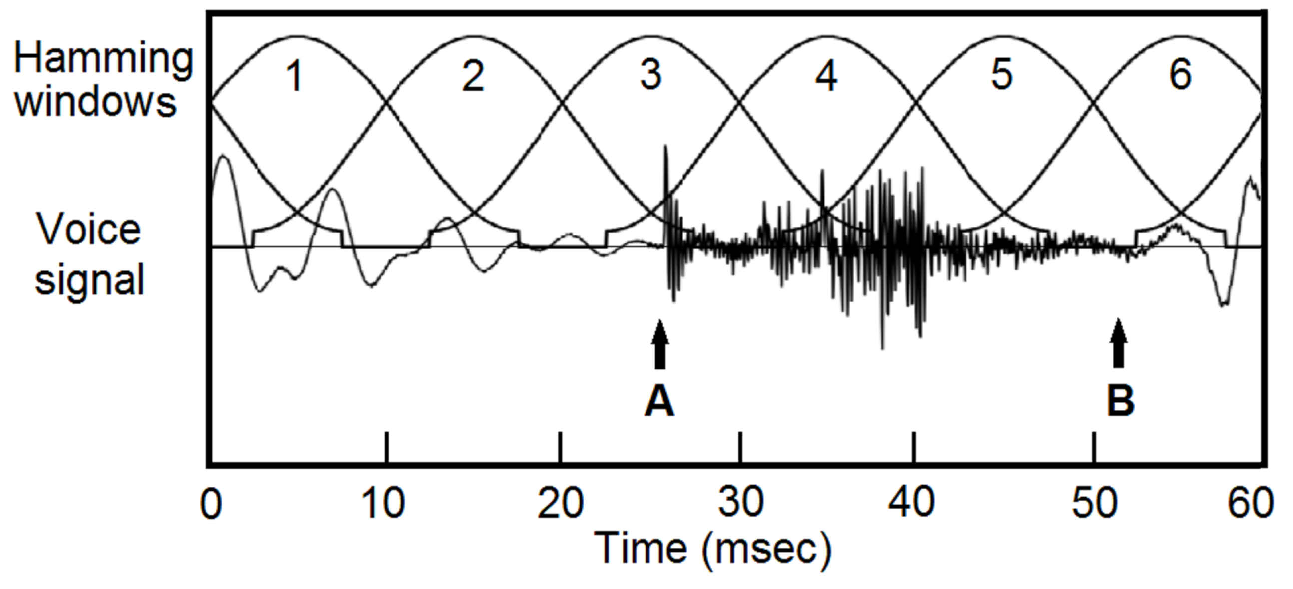
Figure 2.
Dependence of formant frequencies on order p of LPC. To measure formants using LPC, the order of transfer function p is a necessary input parameter. The number and frequencies of formants depend on p. After Fig 8.18 on page 438 of Rabiner and Schafer [10].
Figure 2.
Dependence of formant frequencies on order p of LPC. To measure formants using LPC, the order of transfer function p is a necessary input parameter. The number and frequencies of formants depend on p. After Fig 8.18 on page 438 of Rabiner and Schafer [10].
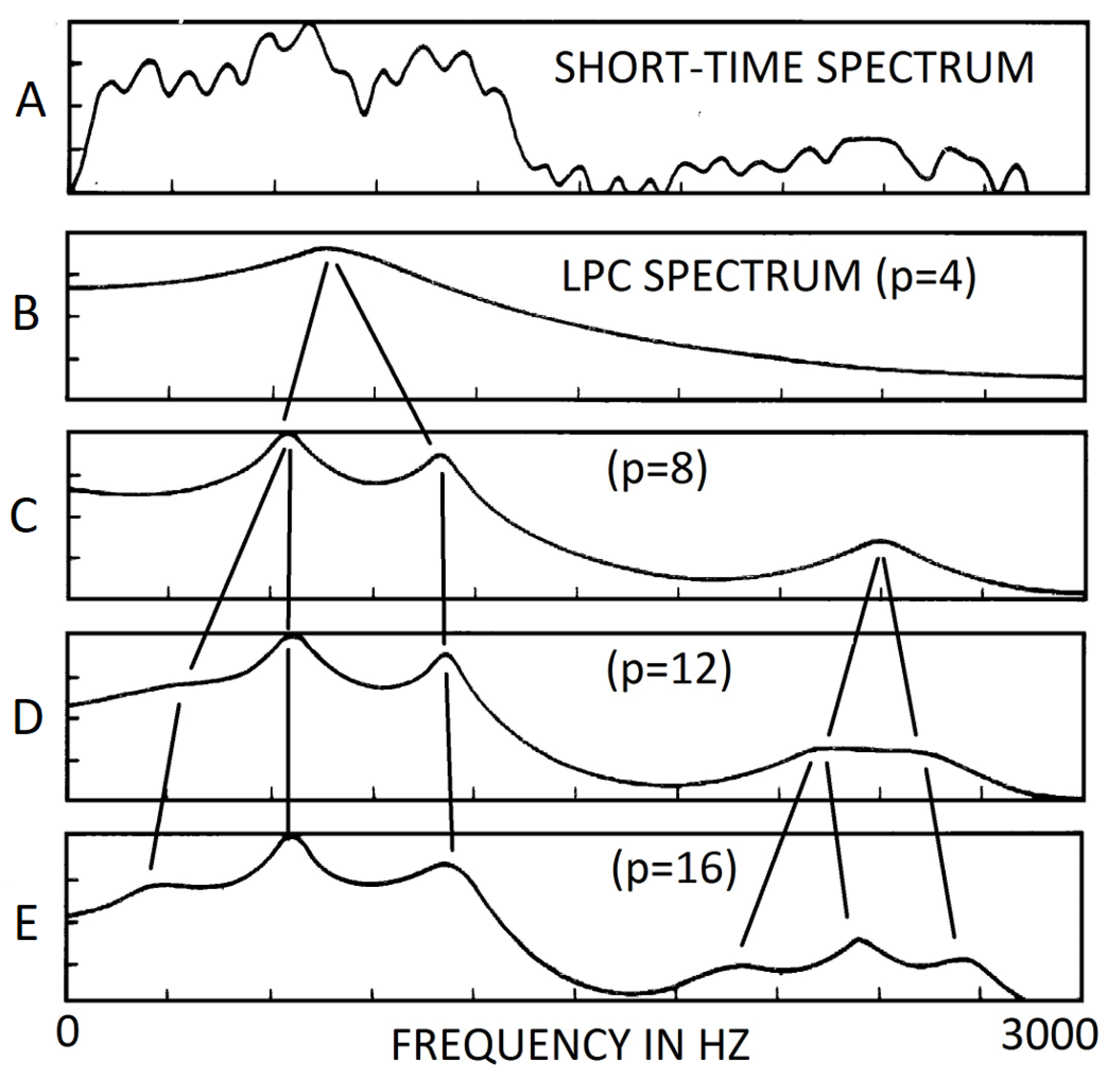
Figure 3.
Mel-scaled triangular windows. The human perception of frequency scale is non-linear. To build MFCC, a set of triangular windows of non-linear scale is multiplied to the spectrum, to generate a set of coefficients.
Figure 3.
Mel-scaled triangular windows. The human perception of frequency scale is non-linear. To build MFCC, a set of triangular windows of non-linear scale is multiplied to the spectrum, to generate a set of coefficients.
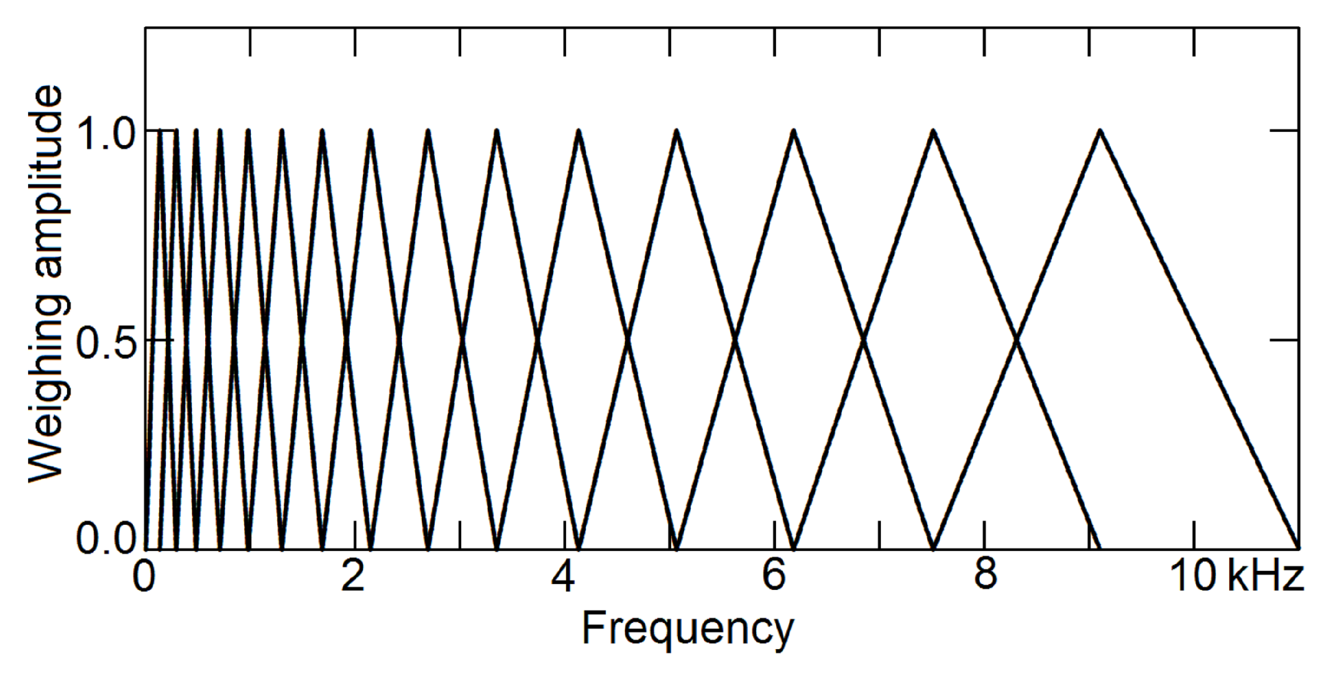
Figure 4.
A schematic of the electroglottograph (EGG). A high-frequency ac signal is applied on one side of the neck. An ac microammeter is connected to an electrode placed on the other side of the neck. (a), an open glottis reduces ac current. (b), a closed glottis increases the ac current. Glottal closing instants can be accurately detected.
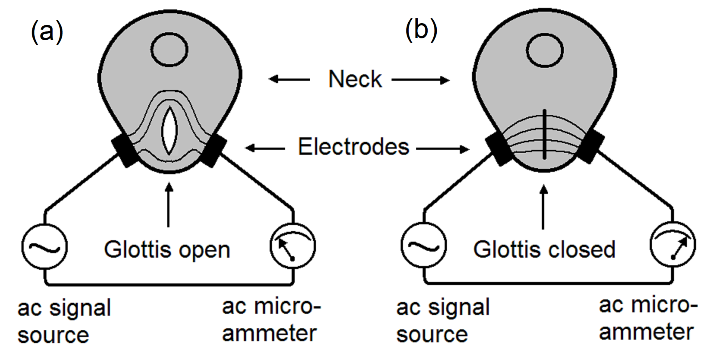
Figure 5.
Temporal correlation between the voice signal and the EGG signal. (a). Immediately after a glottis closing, there is a strong impulse of negative perturbation pressure. (b). In the closed phase of glottis, the voice signal is strong and decaying. (c). The voice signal in the open phase of the glottis is much weaker. (d). Immediately before a glottal closing, there is a peak of positive perturbation pressure, a remnant the glottal flow. See the Preface and Section 3.2 of Reference [20].
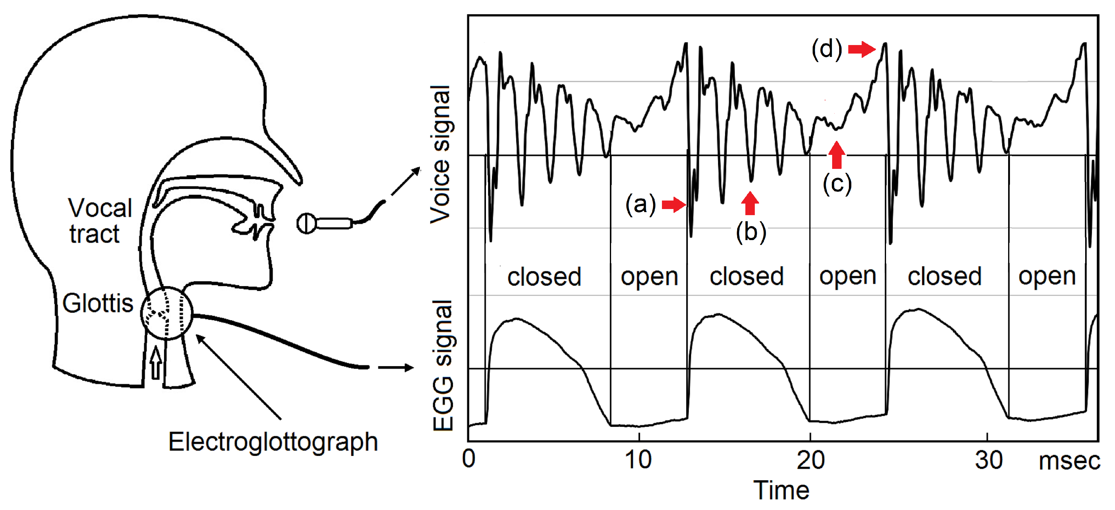
Figure 6.
Mechanism of timbron production. (0), while the glottis is open, there is a steady airflow from the lungs to the vocal tract. No sound is produced. (1), a glottal closing blocks the air flow from the trachea to the vocal track. It creates a negative-pressure wavefront moving towards the lips at the speed of sound and resonates in the vocal tract to become a timbron. See references [18,19,20].
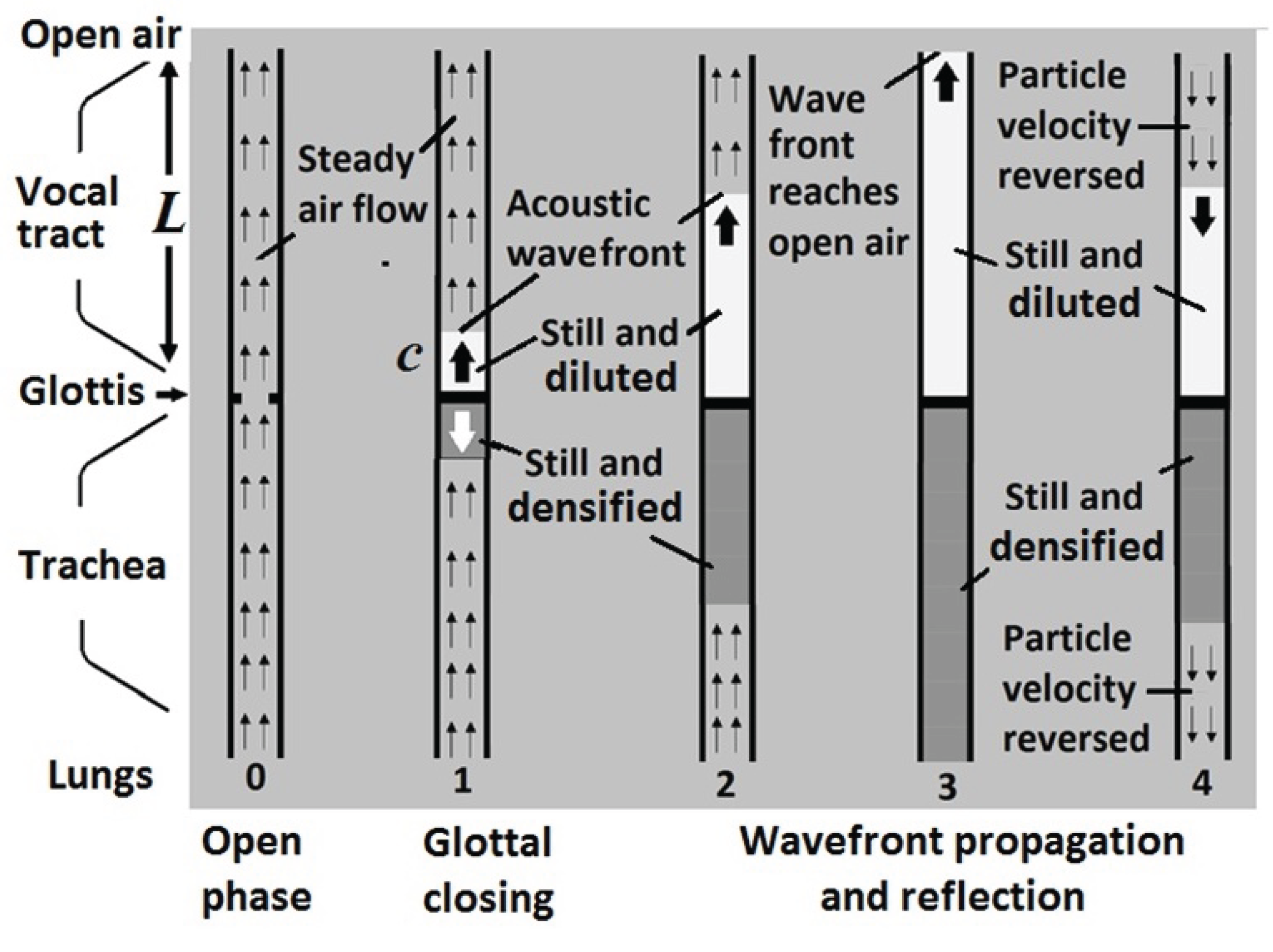
Figure 7.
Superposition of timbrons to become a sustaining voice. (a) through (c), with a series of glottal closings, the timbrons started from those GCIs superpose over each other to become sustaining voice. Each new timbron is adding to the tails of the previous timbrons. Different GCI repetition rates make different pitch frequencies. (d), = 125 Hz. (e), = 100 Hz. (e), = 75 Hz.[18,19,20]
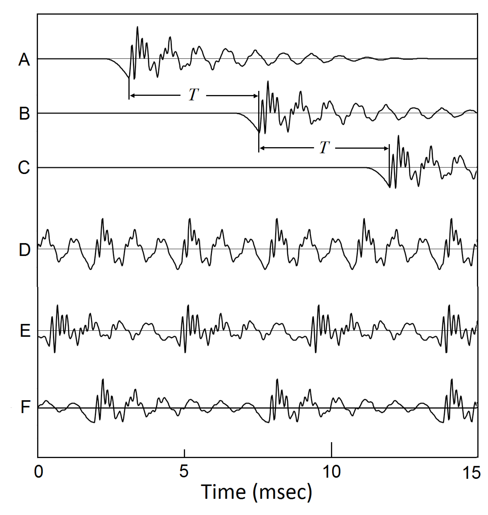
Figure 8.
Segmenting voice signals into pitch periods. A section of sentence a0329 by speaker bdl. At each glottal closing instant (GCI), the dEGG/dt signal shows a sharp peak. Using those GCI points as segmentation points, the voice signal can be segmented into pitch periods.
Figure 8.
Segmenting voice signals into pitch periods. A section of sentence a0329 by speaker bdl. At each glottal closing instant (GCI), the dEGG/dt signal shows a sharp peak. Using those GCI points as segmentation points, the voice signal can be segmented into pitch periods.
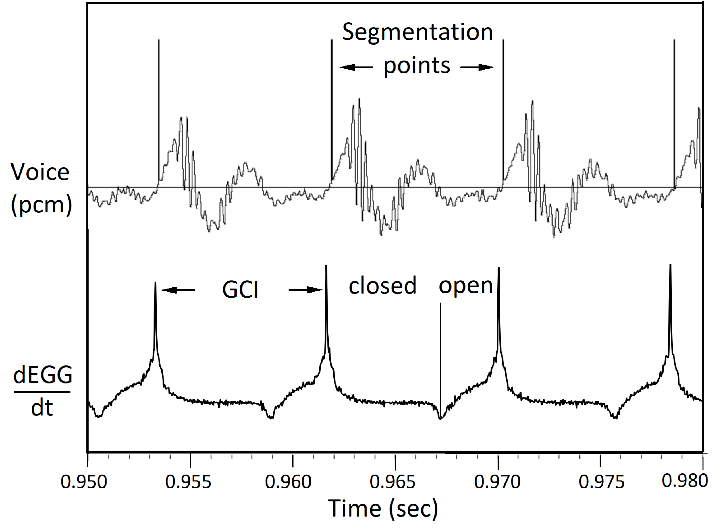
Figure 9.
The ends-matching procedure. (a) The starting value A of a pitch period may be not equal to the ending value C. By taking more points after the end, for example 10 points, CD, making a linear combination with the first 10 points AB and then replace the first 10 points with it. (b). The beginning and the end of a pitch period becomes equal, suitable for Fourier analysis. See references [20,21].
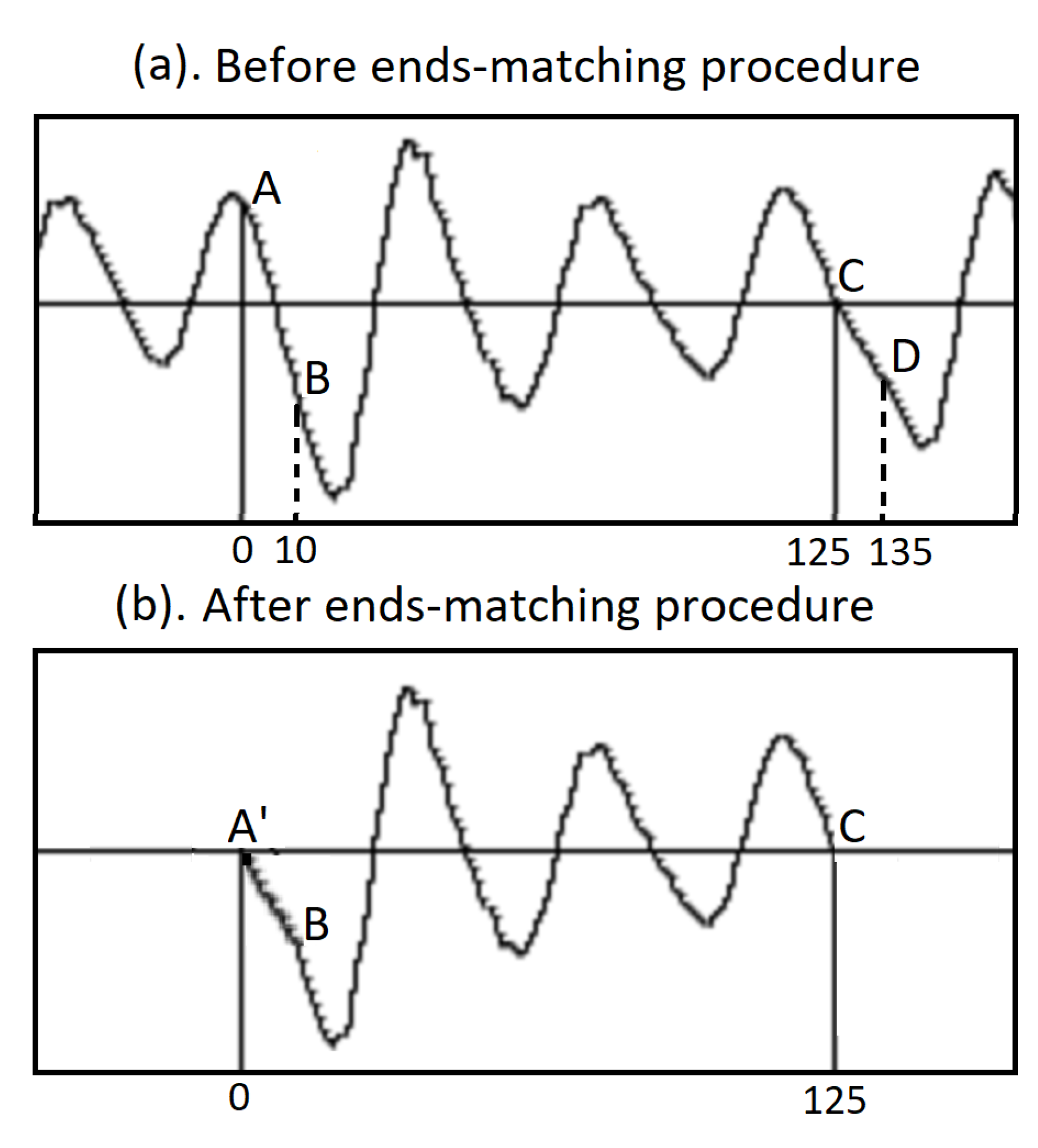
Figure 10.
Amplitude spectra and formants of 10 US English monophthong vowels. Blue dotted curves show the original amplitude spectra from individual pitch periods. Red solid curves show the amplitude spectra recovered from the formant data. For clarity, the curves of formants are represented by Gaussian functions.
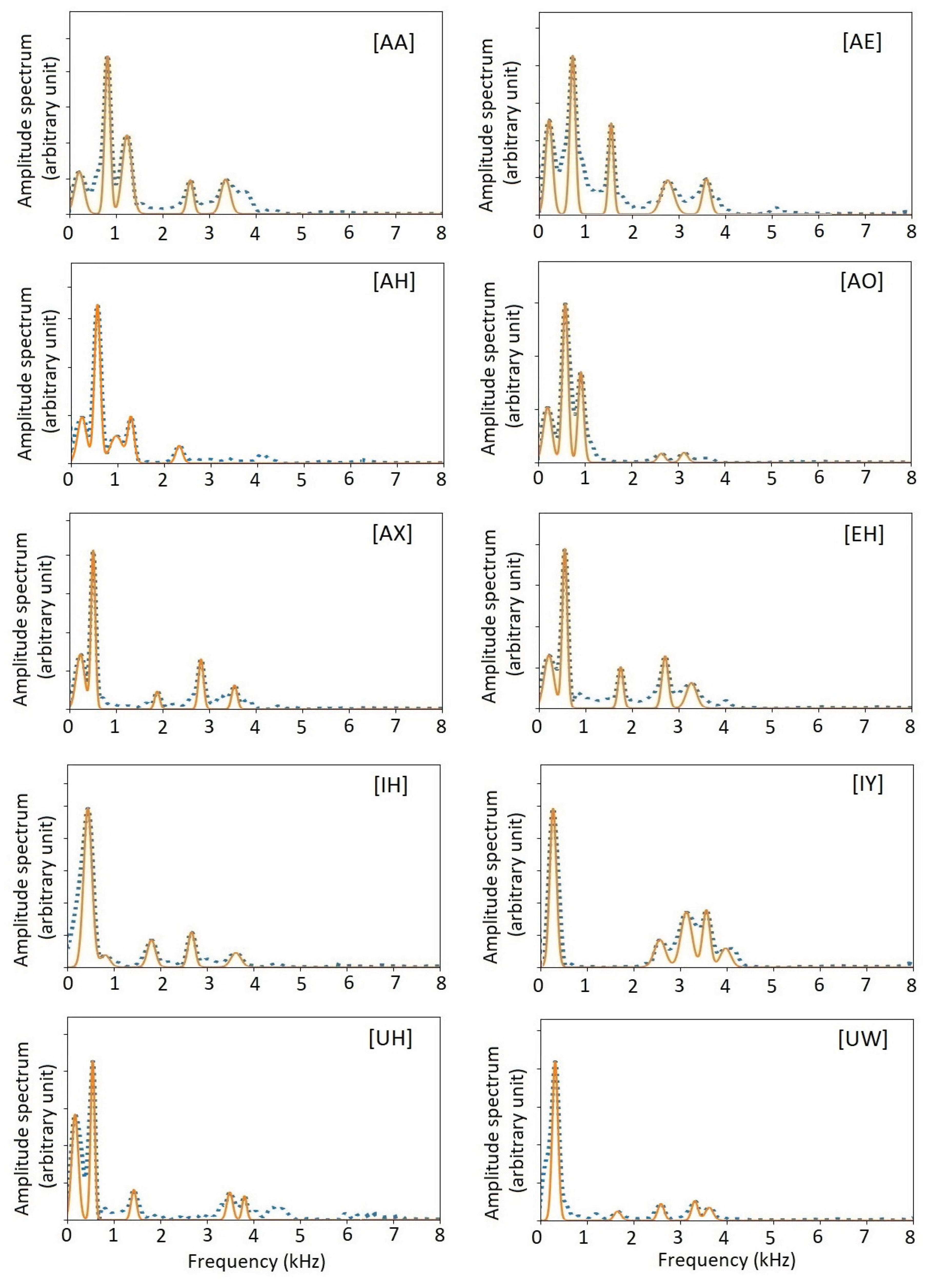
Figure 11.
Laguerre functions. The analytic version of the Mel frequency scale. The first few Laguerre functions describe the gross features of the low-frequency amplitude spectrum. The later Laguerre functions represent the high-frequency spectrum and refine the low-frequency spectrum [32].
Figure 11.
Laguerre functions. The analytic version of the Mel frequency scale. The first few Laguerre functions describe the gross features of the low-frequency amplitude spectrum. The later Laguerre functions represent the high-frequency spectrum and refine the low-frequency spectrum [32].
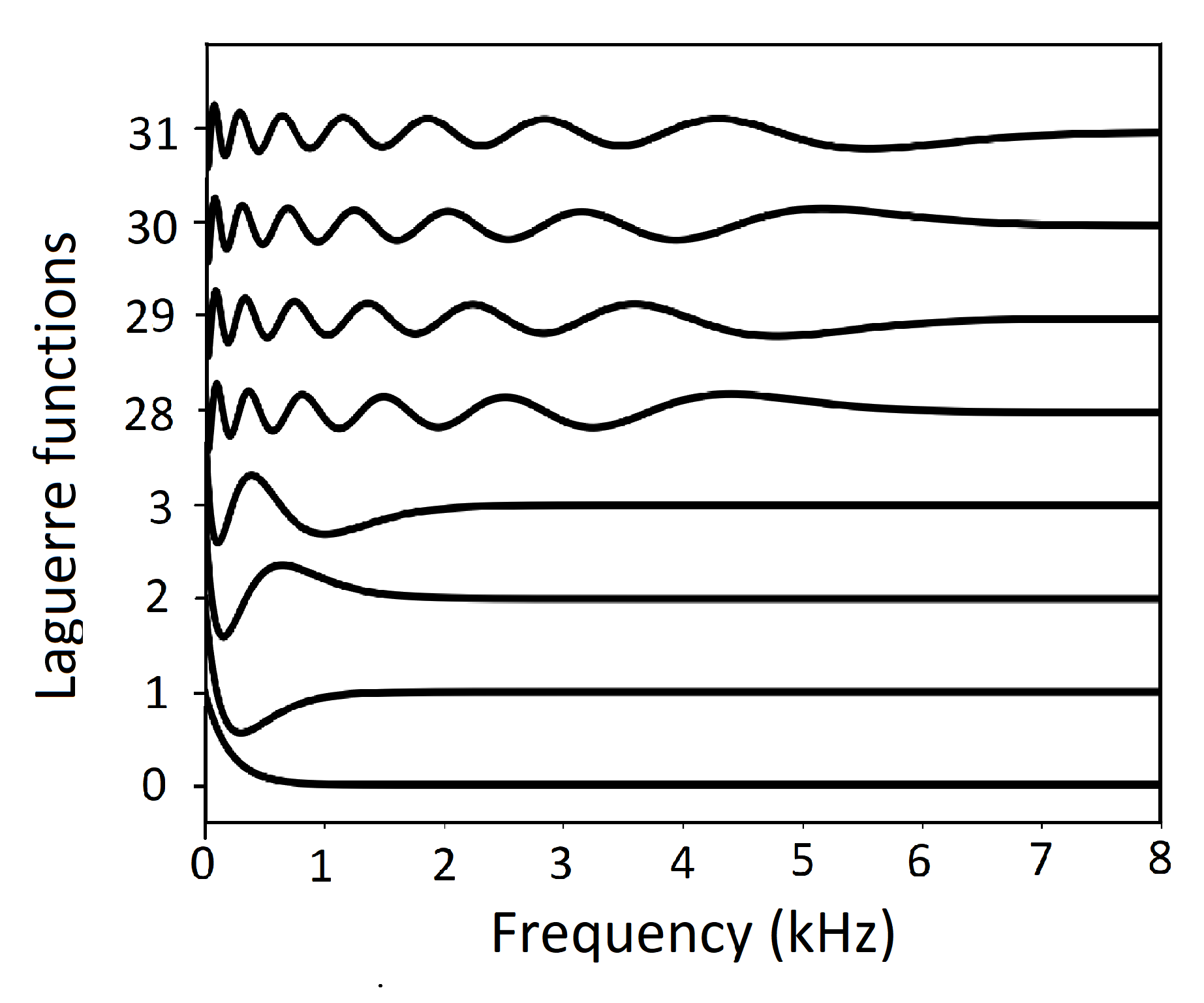
Figure 12.
Amplitude spectra of 10 US English monophthong vowels. Blue dotted curves show the original amplitude spectra from individual pitch periods. Red solid curves show the amplitude spectra recovered from a timbre-vector expansion. Following the Mel curve of human perception, the resolution at lower frequencies is finer than at higher frequencies.
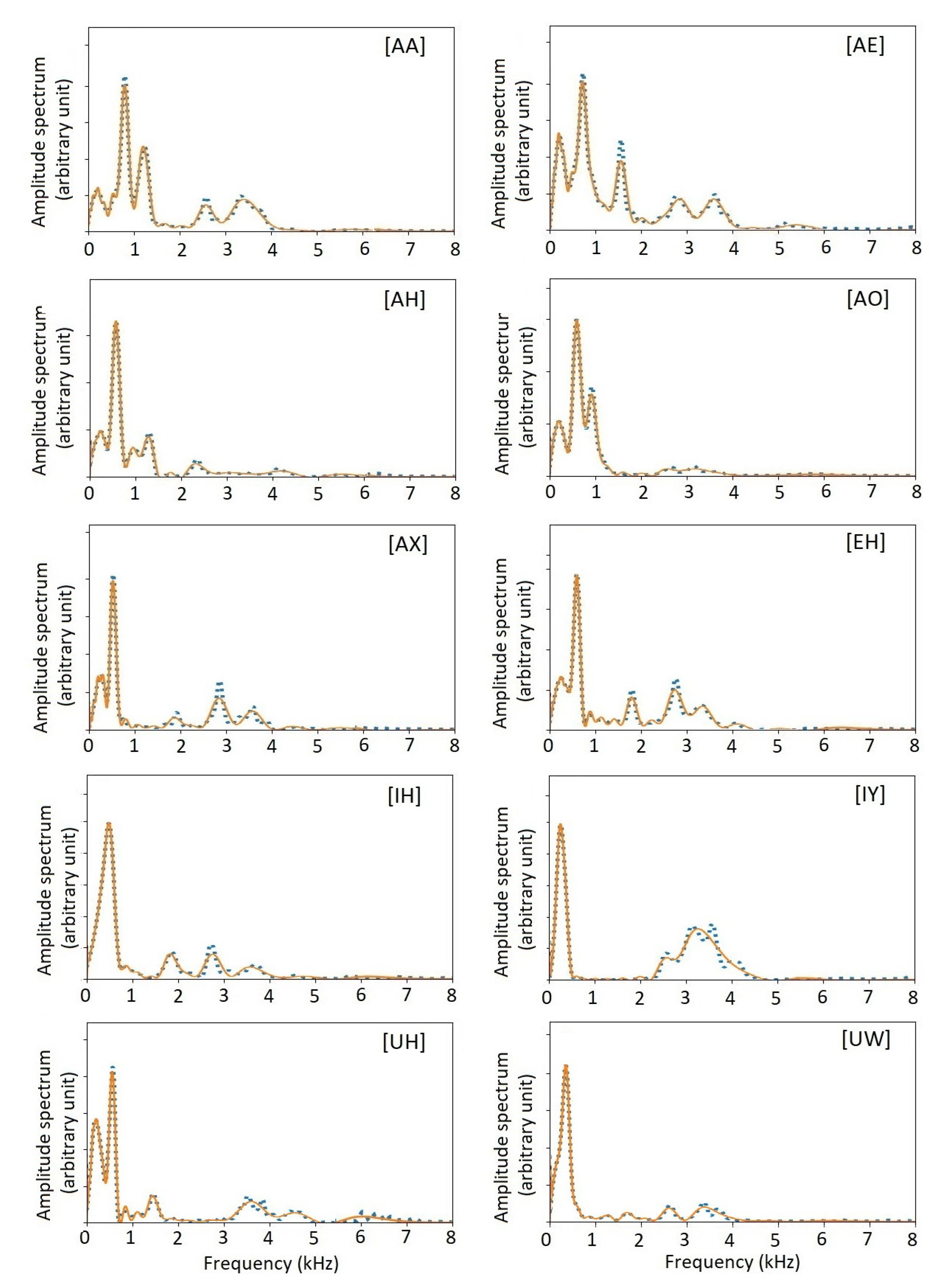
Figure 13.
Timbre vectors from the voice recordings in the Saarbrücken database. (a) the derivatives of EGG, showing sharp peaks at the GCIs. (b) waveforms, a nearly perfect repetition over all pitch periods. (c) amplitude spectra in blue dotted curves, and that recovered from the timbre vectors in red curves. For each vowel, the amplitude spectra in all pitch periods are very similar.
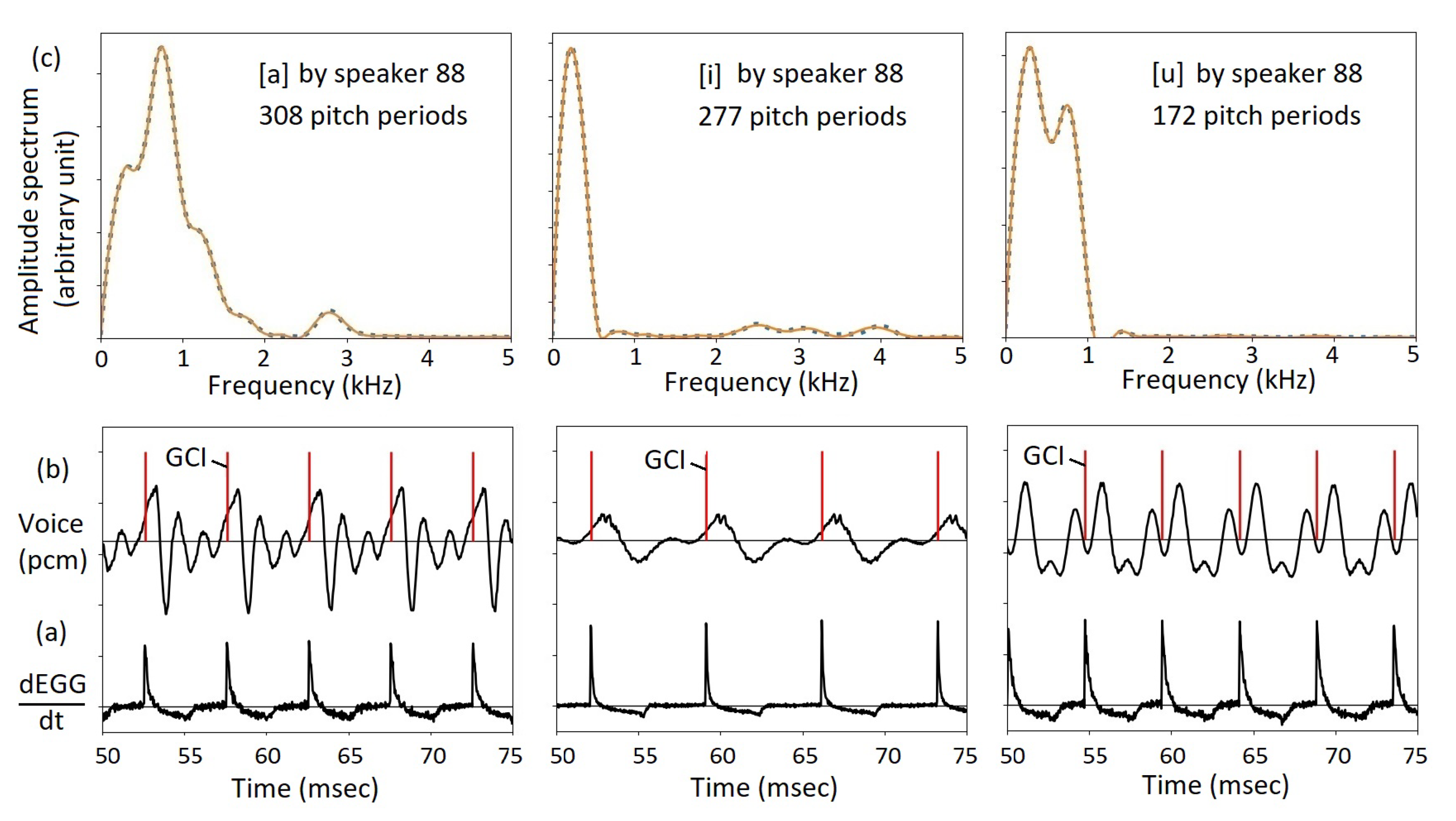
Figure 14.
Measurement of jitter and shimmer (a). Typical method of measuring jitter and shimmer is to investigate the peaks in the voice waveforms by a dedicated software, which is not reliable. (b). for some vowels such as [IY] and [EH], the waveform has multiple peaks, and the determination of the pitch period is compromised. (c), for other vowels such as [OH] and [UW], there are no sharp peaks in the voice waveform, and the determination of the pitch period is also compromised.
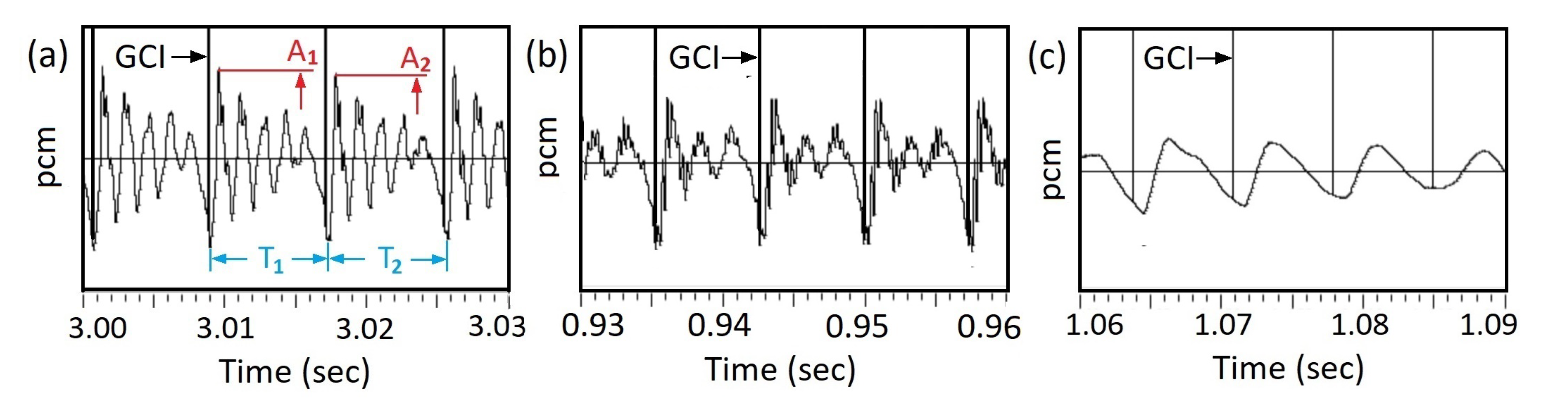
Figure 15.
Asymmetric window for detecting GCI. By convoluting the derivative of the voice signal with an asymmetric window, a profile function is generated. The peaks in the profile function point to GCIs. See Figure 16.
Figure 15.
Asymmetric window for detecting GCI. By convoluting the derivative of the voice signal with an asymmetric window, a profile function is generated. The peaks in the profile function point to GCIs. See Figure 16.
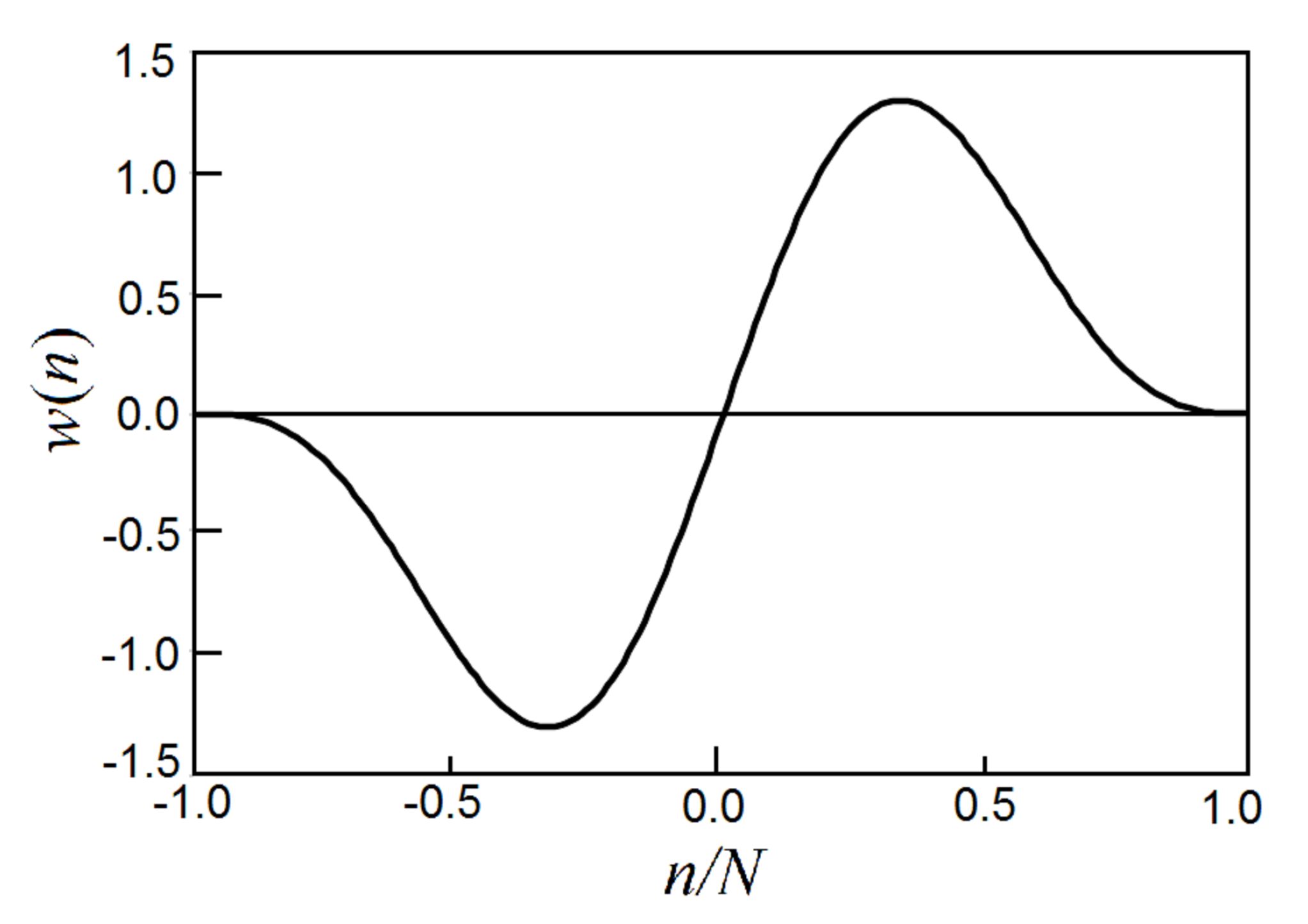
Figure 16.
Profile function for detecting GCIs from the sound wave. An example of the profile function generated by convoluting the derivative of the voice signal with an asymmetric window, shown in Figure 15. The peaks of the profile function, A, are identified as GCIs.
Figure 16.
Profile function for detecting GCIs from the sound wave. An example of the profile function generated by convoluting the derivative of the voice signal with an asymmetric window, shown in Figure 15. The peaks of the profile function, A, are identified as GCIs.
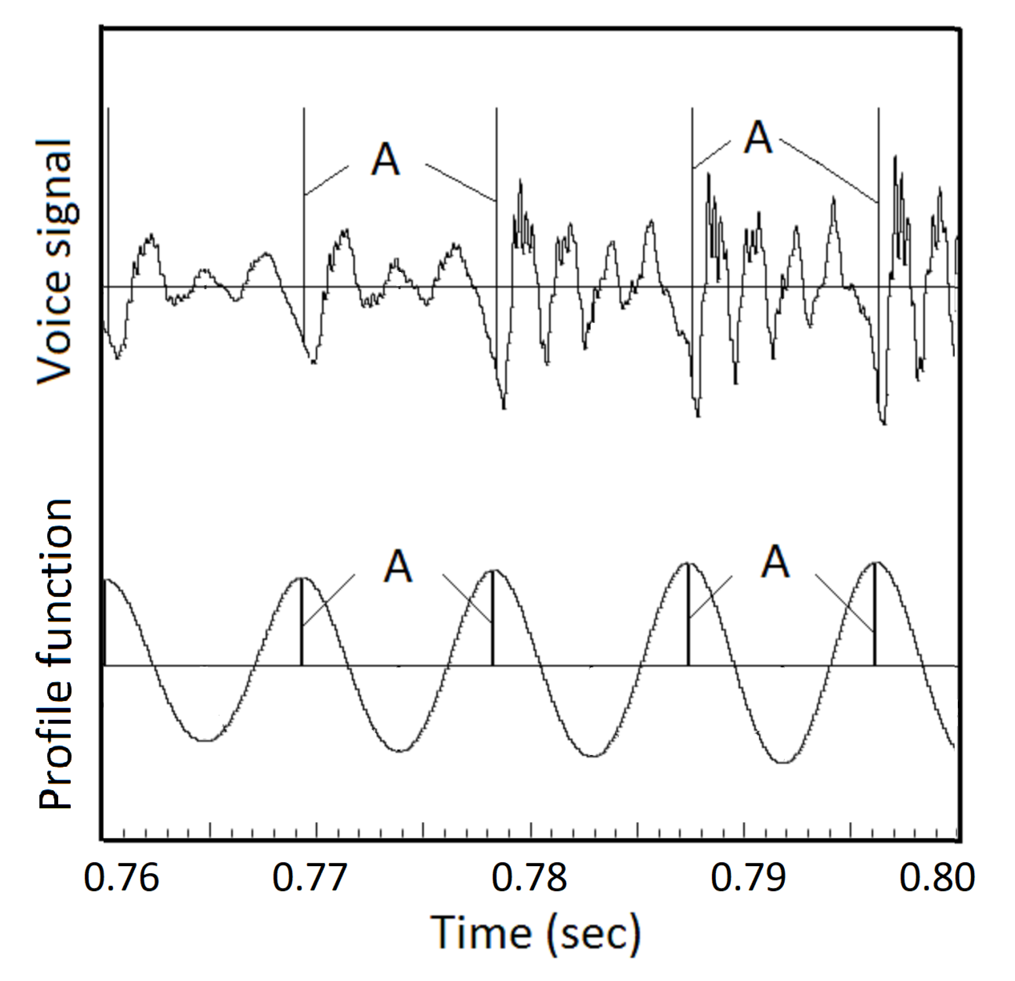
Figure 17.
GCIs detected from voice signals without EGG counterparts. Female speaker slt, sentence b0413, an isolated word “or”. In Section B, there are complete glottal closures. The GCIs detected from voice signals agree well with GCIs from the EGG signals. In sections A and C, the incomplete glottal closures generate voice, which can be detected by the asymmetric window method, but there are no EGG signals. Those extra GCIs are useful for pitch-synchronous signal processing.
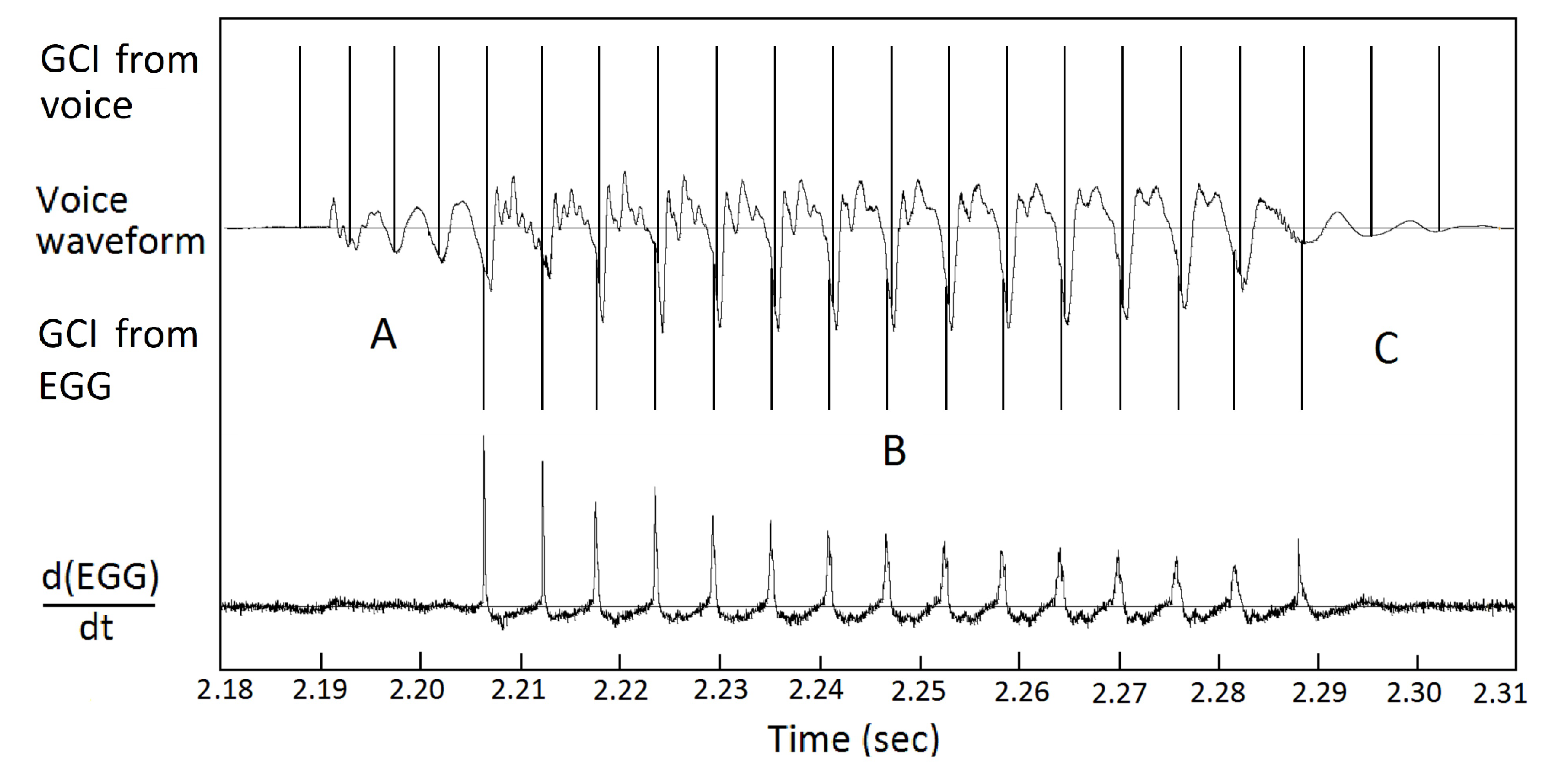

Table 1.
Source of monophthong vowels.
| Vowel | Sentence | Time (sec) | Word |
|---|---|---|---|
| AA | a0329 | 0.36 | Ah |
| AE | b0166 | 0.44 | fast |
| AH | a0207 | 0.52 | much |
| AO | b0357 | 0.45 | law |
| AX | a0388 | 1.20 | idea |
| EH | a0005 | 1.25 | forget |
| IH | a0580 | 0.29 | it |
| IY | a0329 | 0.97 | deed |
| UH | a0158 | 1.16 | good |
| UW | a0102 | 1.37 | soon |
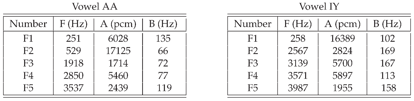
Table 3.
Change of speaker identity in the process of voice synthesis.
| Speaker identity | (Hz) | MIDI | note | |
|---|---|---|---|---|
| Contrabass | 43.7 | 29 | F1 | 1.35 |
| Bass | 61.5 | 35 | B1 | 1.18 |
| Tenor | 123 | 47 | B2 | 1.0 |
| Alto | 175 | 53 | F3 | 0.85 |
| Soprano | 349 | 65 | F4 | 0.75 |
| Child | 494 | 71 | B4 | 0.68 |
Table 4.
Timbre distances among US English monophthong vowels
| AA | AE | AH | AO | AX | EH | IH | IY | UH | UW | |
|---|---|---|---|---|---|---|---|---|---|---|
| AA | 0.000 | 0.453 | 0.939 | 0.719 | 1.219 | 1.032 | 1.246 | 1.214 | 1.102 | 1.297 |
| AE | 0.453 | 0.000 | 0.631 | 0.411 | 0.806 | 0.579 | 0.810 | 0.938 | 0.617 | 0.948 |
| AH | 0.939 | 0.631 | 0.000 | 0.183 | 0.436 | 0.211 | 0.515 | 1.335 | 0.269 | 1.106 |
| AO | 0.719 | 0.411 | 0.183 | 0.000 | 0.654 | 0.334 | 0.698 | 1.339 | 0.445 | 1.178 |
| AX | 1.219 | 0.806 | 0.436 | 0.654 | 0.000 | 0.305 | 0.191 | 0.962 | 0.290 | 0.861 |
| EH | 1.032 | 0.579 | 0.211 | 0.334 | 0.305 | 0.000 | 0.397 | 1.002 | 0.271 | 0.943 |
| IH | 1.246 | 0.810 | 0.515 | 0.698 | 0.191 | 0.397 | 0.000 | 0.896 | 0.354 | 0.436 |
| IY | 1.214 | 0.938 | 1.335 | 1.339 | 0.962 | 1.002 | 0.896 | 0.000 | 0.747 | 0.381 |
| UH | 1.102 | 0.617 | 0.269 | 0.445 | 0.290 | 0.271 | 0.354 | 0.747 | 0.000 | 0.653 |
| UW | 1.297 | 0.948 | 1.106 | 1.178 | 0.861 | 0.943 | 0.436 | 0.381 | 0.653 | 0.000 |
Table 5.
Jitter, shimmer, and spectral irregularity based on the GCI values derived from EGG signals.
Table 5.
Jitter, shimmer, and spectral irregularity based on the GCI values derived from EGG signals.
| Vowel | Number of periods | Jitter percent | Shimmer dB | Spectral irregularity |
|---|---|---|---|---|
| a | 308 | 0.652 | 0.197 | 0.376 |
| i | 277 | 0.401 | 0.089 | 0.070 |
| u | 172 | 0.576 | 0.235 | 0.250 |
Table 6.
Jitter, shimmer, and spectral irregularity based on the GCI values derived from voice signals.
Table 6.
Jitter, shimmer, and spectral irregularity based on the GCI values derived from voice signals.
| Vowel | Number of periods | Jitter percent | Shimmer dB | Spectral irregularity |
|---|---|---|---|---|
| a | 308 | 0.320 | 0.194 | 0.324 |
| i | 277 | 0.258 | 0.083 | 0.088 |
| u | 172 | 0.475 | 0.220 | 0.396 |
Table 7.
Comparison of GCIs from EGG and GCIs from WAV.
| Speaker | bdl | slt |
|---|---|---|
| Number of GCIs from EGG | 247538 | 368864 |
| Number of GCIs from WAV | 279962 | 411471 |
| GCIs from EGG not in WAV | 2190 | 4028 |
| Percentage of the above | 0.88% | 1.09% |
| GCIs from WAV not in EGG | 35753 | 47784 |
| Percentage of the above | 12.77% | 11.61% |
Disclaimer/Publisher’s Note: The statements, opinions and data contained in all publications are solely those of the individual author(s) and contributor(s) and not of MDPI and/or the editor(s). MDPI and/or the editor(s) disclaim responsibility for any injury to people or property resulting from any ideas, methods, instructions or products referred to in the content. |
© 2025 by the authors. Licensee MDPI, Basel, Switzerland. This article is an open access article distributed under the terms and conditions of the Creative Commons Attribution (CC BY) license (http://creativecommons.org/licenses/by/4.0/).
Copyright: This open access article is published under a Creative Commons CC BY 4.0 license, which permit the free download, distribution, and reuse, provided that the author and preprint are cited in any reuse.


