Submitted:
22 December 2025
Posted:
23 December 2025
You are already at the latest version
Abstract
Accurate field-scale meteorological information is required for precision agriculture, but operational numerical weather prediction products remain spatially coarse and cannot resolve local microclimate variability. This study proposes a data-fusion superresolution workflow that combines global GFS predictors (0.25°), regional station observations from southern Moravia (Czech Republic), and static physiographic descriptors (elevation and terrain gradients) to predict 24 h ahead 2 m air temperature and to generate spatially continuous high-resolution temperature fields. Several model families (LightGBM, TabPFN, Transformer, and Bayesian Neural Fields) are evaluated under spatiotemporal splits designed to test generalization to unseen time periods and unseen stations; spatial mapping is implemented via a KNN interpolation layer in physiographic feature space. All learned configurations reduce mean absolute error relative to raw GFS across splits. In the most operationally relevant regime (unseen stations and unseen future period), TabPFN–KNN achieves the lowest MAE (1.26 °C), corresponding to an ≈24% reduction versus GFS (1.66 °C). The results support the feasibility of an operational, sensor-infrastructure-compatible pipeline for high-resolution temperature superresolution in agricultural landscapes.
Keywords:
precision agriculture
; weather downscaling
; super-resolution
; data fusion
; near-surface air temperature
; Global Forecast System (GFS)
; ERA5-Land
; sensor networks
; TabPFN
; k-nearest neighbours (KNN)
1. Introduction
Global food systems face increasing pressure from climate change and population growth. The world population is projected to reach 9.7 billion by 2050 [1], while climate change is associated with increased variability and a higher frequency of extreme weather events [2]. These trends increase the demand for accurate, spatially detailed meteorological information that can support risk-aware planning in agriculture. Precision agriculture frameworks underline that site-specific weather and microclimate information is a prerequisite for optimizing inputs, reducing environmental impacts, and stabilizing yields [3,4,5].
Operational numerical weather prediction (NWP) models such as the Global Forecast System (GFS) provide global coverage and multi-variable forecasts at regular update cycles. However, they operate at horizontal resolutions on the order of tens of kilometres; for example, standard GFS configurations use a grid spacing of approximately 25–28 km [6]. At this scale, important microclimatic variations driven by local topography, land cover, and surface heterogeneity are not resolved. Within a single NWP grid cell, precipitation, temperature, and humidity can differ substantially between slopes, valleys, and plateaus [7]. Consequently, raw NWP products are often too coarse to directly support field-scale decision-making in agriculture.
Local meteorological stations and dedicated agricultural weather networks partially compensate for this limitation. Standardized in situ measurements provide accurate point data for key variables such as air temperature, humidity, wind, and precipitation [8]. Agricultural meteorological networks and farm-scale monitoring systems extend this capability to specific crops and production systems [9]. Nevertheless, the spatial density of such stations is generally limited by installation and maintenance costs, and the available networks frequently provide monitoring rather than dedicated forecasting products. As a result, there is a gap between coarse-grid forecasts and the high-resolution weather information required at field scale.
Hybrid data-driven approaches aim to bridge this gap by combining global model outputs, reanalysis products, and station observations. Quality-controlled station archives such as HadISD provide sub-daily time series from thousands of stations worldwide, including long-term records from Central Europe [10,11]. Global reanalysis products such as ERA5 and its land-focused derivative ERA5-Land offer physically consistent gridded data at higher spatial resolution than operational NWP, produced by assimilating in situ and remote sensing observations into numerical models [12,13]. The use of multi-source observations and data assimilation has led to significant improvements in large-scale land–atmosphere representation [14]. For local forecasting and downscaling, these datasets can be used either as direct predictors, as high-resolution targets for supervised learning, or as auxiliary sources that encode information about conditions in the surroundings of a station.
In previous work, we investigated the combination of local weather station data with global forecasts and reanalysis to improve 24 h ahead predictions at station locations in the Czech Republic [15]. HadISD station data from 27 sites were combined with GFS forecasts on a 0.25° grid and ERA5-Land reanalysis used as an additional source of spatial context. Multilayer perceptrons, CatBoost gradient-boosting models, and long short-term memory (LSTM) neural networks were evaluated, and a U-Net-based model was trained to approximate ERA5-Land fields from GFS inputs, providing a high-resolution proxy in near real time. The results showed that integrating station measurements with GFS outputs significantly reduced forecast error compared to GFS alone, confirming the potential of hybrid local–global methods for agricultural applications.
Recent advances in machine learning provide a suitable methodological framework for such hybrid systems. Deep learning has become a standard tool for modelling high-dimensional, nonlinear relationships in large datasets [16]. In meteorology, hybrid deep models have been used for short-term forecasting of temperature and precipitation [17,18]. Gradient-boosting methods such as CatBoost and LightGBM have demonstrated strong performance in tabular regression tasks relevant to weather prediction, especially with heterogeneous predictor sets [19,20]. Dedicated spatio-temporal architectures, including convolutional neural network–LSTM hybrids and temporal convolutional networks, have been proposed for station-based time series and local weather variables [21,22]. Statistical approaches using copulas address multivariate dependence structures in hydro-meteorological extremes [23], while convolutional networks have been successfully applied to detect extreme events in gridded climate reanalyses [24]. At the scale of climate and NWP ensembles, machine learning has been shown to improve predictive skill by post-processing and refining coarse model outputs [25].
Beyond point predictions, considerable effort has been devoted to exploiting machine learning for spatial downscaling and superresolution of Earth system data. Deep learning has been used both to emulate subgrid-scale processes in climate models and to reconstruct fine-scale spatial patterns from coarse inputs [26,27]. Single-image superresolution approaches such as DeepSD have been applied to climate projections, demonstrating that convolutional encoder–decoder architectures can recover high-resolution fields from low-resolution climate information [28]. Deep-learning-based gridded downscaling methods for surface meteorological variables in complex terrain further confirm that such architectures can handle strong orographic effects [29]. Enhanced residual U-Net designs have been proposed for temporal and spatial downscaling of gridded geophysical data [30], building on the original U-Net architecture developed for image segmentation [31]. More recently, superresolution methods have been applied directly to global weather forecasts [32], showing that operational NWP outputs can be post-processed into higher-resolution fields with improved representation of local structures.
These developments are closely connected to precision agriculture, where wireless sensor networks, Internet-of-Things infrastructures, and decision-support systems are used to link environmental observations to crop and farm management [3,33,34,35]. Weather- and climate-informed decision-making is central to many precision agriculture applications, including frost protection, irrigation scheduling, disease risk modelling, and harvest logistics. Several recent studies explicitly combine machine learning–based forecasting with agricultural advisory use cases, for example in digital agriculture platforms and regional decision-support systems [35,36]. However, many existing systems remain limited either to station-level forecasts or to coarse-grid NWP products, without providing spatially continuous, high-resolution fields at scales directly relevant to fields and plots.
Operational deployment of such methods requires not only robust predictive models but also sensor data infrastructures that can ingest, harmonize, and disseminate data from multiple networks. The SensLog platform was proposed as a general solution for managing heterogeneous sensor data, including environmental and citizen observatory measurements [37,38]. SensLog provides functionality for registering sensors, handling different communication protocols, storing time series, and exposing them through standardized interfaces. It has been applied in several environmental and agricultural contexts and is suitable as the data-management backbone for machine-learning-based forecasting services that need to handle distributed station networks.
The present work extends our previous station-level hybrid forecast framework [15] towards explicit spatial superresolution of weather data for precision agriculture. We focus on near-surface air temperature, which is a primary driver for many agricultural processes and a key variable for frost risk. Building on publicly available GFS forecasts, ERA5-Land reanalysis, high-resolution topographic data, and dense agricultural weather station networks, we construct a data fusion pipeline that produces sub-kilometre temperature fields. Machine learning models are trained to map from coarse NWP predictors, reanalysis-based proxies, static geographical descriptors, and station observations to high-resolution temperature estimates, following recent advances in gradient boosting and deep neural architectures for geoscientific data [19,20,21,22,26,27,28,29,30,31,32]. The resulting framework is designed to be integrated with SensLog [37,38] and other operational services, enabling practical deployment of superresolved weather information into agricultural decision-support chains.
Research goals and hypotheses
This study is designed to test whether super-resolution and data fusion can deliver operationally useful, field-scale meteorological information for precision agriculture when driven by routinely available forecast and sensor inputs. The work is structured around the following research goals (RG) and hypotheses (H), which are evaluated in subsequent sections.
RG1 (Field-scale super-resolution target): Develop an operational pipeline that produces spatially continuous, high-resolution (sub-kilometre to kilometre-scale) near-surface air temperature fields for agricultural decision support from routinely available sources (global NWP, reanalysis-derived proxies, static physiographic predictors, and station observations).
RG2 (Multi-source data fusion): Quantify the incremental contribution of (i) local station observations, (ii) high-resolution reanalysis proxies, and (iii) static geographic descriptors (elevation, slope, aspect, land cover) to super-resolved temperature skill relative to a baseline using global NWP alone.
RG3 (Infrastructure and deployability): Implement and assess an end-to-end data handling workflow in which sensor observations are ingested, quality controlled, and served through a sensor platform (SensLog) for model training and near-real-time inference.
H1 (Skill improvement vs. coarse NWP): Super-resolution models conditioned on global NWP predictors will significantly reduce near-surface air temperature error at independent station locations compared with raw NWP values sampled at the station grid cell.
H2 (Value of local observations): Incorporating local station observations (or station-informed features) into the fusion model will yield statistically significant additional error reduction beyond NWP-only and NWP+proxy configurations, particularly under stable boundary-layer conditions (e.g., nocturnal inversions) when microclimate effects are strongest.
H3 (Value of reanalysis proxy features): Adding a high-resolution proxy field derived from reanalysis (or a learned approximation thereof) will improve spatial pattern reconstruction and reduce spatially structured residuals compared with using NWP predictors and static physiography alone.
H4 (Role of physiography): Static physiographic predictors (elevation and terrain derivatives) will be necessary to capture systematic, location-dependent biases and to stabilize model generalization when extrapolating across heterogeneous landscapes.
H5 (Operational robustness): The proposed workflow will maintain stable prediction skill over multiple seasons and will remain functional under realistic station availability constraints (missingness, heterogeneous sampling intervals), enabling deployment within SensLog-supported infrastructures.
These goals and hypotheses establish a testable structure for the remainder of the manuscript: baseline definition and datasets (Methods), super-resolution model formulation and ablation studies (Methods/Results), statistical verification and robustness checks (Results), and integration aspects with the sensor platform (System/Implementation)..
2. Materials and Methods
2.1. Study Area
The experiments were conducted in the wine-growing region of southern Moravia (Czech Republic). This area is characterized by gently undulating terrain with elevations typically between 150 and 400 m a.s.l., heterogeneous land use dominated by vineyards and arable land, and pronounced microclimatic variability driven by local topography (valleys, slopes, plateaus). To ensure sufficient spatial sampling of these microclimatic gradients, we used a dense network of automated agricultural weather stations operated by the National Wine Growers’ Association (EKOVÍN). The final dataset includes 36 stations selected based on temporal completeness, sensor calibration quality, and spatial representativeness within the region (Figure 1).
The stations record near-surface air temperature at 15-minute intervals, which allows us to resolve diurnal cycles and short-lived events such as nocturnal inversions and advective cold-air drainage. Additional variables (relative humidity, precipitation, leaf wetness, solar radiation) are available at many stations, but for the present work we use them only as auxiliary quality-control information; the target variable for superresolved prediction is 2-m air temperature.
2.2. Data
2.2.1. Numerical Weather Prediction Data (GFS)
As the primary large-scale predictor we use output from the Global Forecast System (GFS), a global numerical weather prediction model with horizontal grid spacing of 0.25° (≈28 km in mid-latitudes) and 6-hourly forecast cycles. From the NCAR Research Data Archive, we extract a set of surface and low-level variables including 2-m air temperature, relative humidity, surface pressure, wind components, precipitation, and shortwave radiation.
These GFS fields serve two roles: (i) they define the baseline reference against which superresolution skill is evaluated, and (ii) they form a core subset of predictors for the machine learning models. For each station and forecast time, we sample the GFS grid cell containing the station and construct feature vectors that combine current and lagged GFS predictors with other inputs described below.
2.2.2. Agricultural Weather Station Network
The vineyard station network provides high-frequency in situ observations used both as training targets and, in some configurations, as autoregressive predictors. Each station is equipped with calibrated sensors for near-surface temperature and other meteorological variables. Raw observations are first passed through the SensLog platform, which provides basic quality control (range checks, detection of missing or obviously erroneous values), time-stamping, and persistent storage in a central database.
For the superresolution experiments, station data are aggregated to an hourly resolution to harmonize with the temporal resolution of the GFS predictors. For each station, we retain only periods with continuous records over the training and validation intervals; stations with substantial gaps or sensor problems are excluded to avoid introducing spurious noise into the learning process.
2.2.3. Static Geographic Data
Static physiographic predictors provide spatial context that is essential for representing topographically induced temperature patterns at sub-kilometre scales. For each station and for each target grid cell in the high-resolution prediction lattice, we derive:
- Latitude and longitude;
- Elevation from the ASTER Global Digital Elevation Model at 500 m resolution;
- North–south and east–west elevation gradients computed by finite differences, used to represent slope magnitude and aspect-related effects.
These static features enable the models to learn systematic temperature differences between, for example, valley bottoms and surrounding slopes, or between north- and south-facing slopes, and are also used as inputs in the K-Nearest Neighbour (KNN) interpolation stage (Section 2.4.4).
2.2.4. Data Integration and Feature Construction
All dynamic and static sources are integrated into a common tabular representation. For each station–time pair used in training or validation, we construct a feature vector consisting of:
- Station-based predictors: recent temperature history and, where available, other meteorological variables aggregated over the preceding hours;
- GFS-based predictors: the full set of selected surface and low-level fields at the station grid cell, optionally including derived features such as helicity, minimum temperature above ground, and precipitable water;
- Static physiographic descriptors: elevation and slope components as described above.
A preliminary feature importance analysis based on CatBoost and SHAP values from our earlier GFS–station fusion work is used to down-select the most informative predictors and reduce dimensionality, while retaining variables known to be relevant for near-surface temperature (e.g., surface temperature, precipitable water, station temperature and dew point).
2.3. Overall System Architecture
2.3.1. Logical Workflow
The overall architecture follows a modular design aligned with the ALIANCE platform. At a high level, the workflow comprises the following stages:
-
Acquisition and ingestion
- ○
- External forecast data (GFS) are downloaded on a rolling basis and stored in a dedicated repository
- ○
- Station measurements are ingested into SensLog through feeder services, which normalize formats and apply basic quality control.
-
Pre-processing and feature assembly
- ○
- A preprocessing layer maps station locations to the GFS grid, merges dynamic predictors with static physiographic attributes, and constructs feature vectors and target values for each station and time step.
- ○
- The same layer prepares a high-resolution prediction grid over the southern Moravia domain by sampling static geographic predictors at the desired spatial resolution.
-
Model training
- ○
- Models are trained using historical data, with different model families evaluated under identical spatiotemporal cross-validation schemes (Section 2.4).
-
Operational inference and superresolution
- ○
- For a given forecast time, a trained model ingest the latest available GFS forecast fields and, where relevant, static attributes to produce 24-hour temperature predictions at the desired resolution.
-
Publication and integration
- ○
- Resulting high-resolution temperature fields and station-level forecasts are stored in SensLog and exposed via standardized APIs so that other ALIANCE components (e.g., localized weather forecast services, crop and risk models) can consume them.
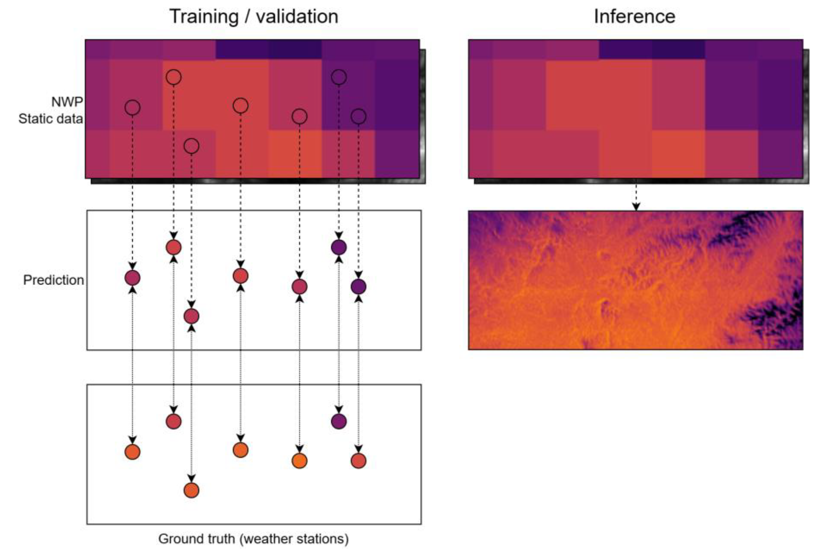
Figure 2.
Method illustration.
2.3.2. Infrastructure Integration
In the ALIANCE infrastructure, SensLog acts as the central data and publication layer for both sensor data and model outputs. Dedicated connector services handle periodic retrieval of external forecasts and orchestrate the flow of data between SensLog, the superresolution models, and downstream applications. This design is consistent with the architecture adopted for the localized forecast and Sentinel-2 reconstruction services, where EO Data API endpoints and forecast APIs provide homogeneous access to heterogeneous model outputs.
2.4. Models
2.4.1. Problem Formulation
The superresolution task is formulated as a supervised regression problem. Given a feature vector xs,tx_{s,t}xs,t constructed from GFS predictors, recent station observations, and static physiographic attributes for station sss and time ttt, the model predicts the 2-m air temperature ys,t+Δy_{s,t+\Delta}ys,t+Δ at horizon Δ=24\Delta = 24Δ=24 h. The objective is to minimize the mean absolute error (MAE) between predictions and observed station temperatures on held-out spatiotemporal subsets.
2.4.2. Base Predictive Model
We evaluate several complementary model families designed for tabular geoscientific data:
- Bayesian Neural Fields (BayesNF)
A spatiotemporal Bayesian neural model that combines deep neural networks with hierarchical Bayesian inference. In this study, we extend its original input space (date–time and coordinates) by including static geographic predictors and selected GFS variables, while retaining MAP estimation and seasonal harmonics tuned to daily and annual cycles.
- LightGBM
A gradient-boosted decision tree model optimized for efficiency and performance on structured data. We employ LightGBM primarily as a strong non-linear tabular baseline to correct systematic GFS biases, using mostly default hyperparameters identified as robust in preliminary experiments.
- TabPFN
A transformer-based Prior-Data Fitted Network pre-trained on synthetic tabular tasks and adapted here for regression. TabPFN allows us to capture complex non-linear relationships between NWP predictors, static geography, and station temperatures without extensive manual feature engineering.
- Transformer for tabular bias correction
A custom transformer architecture for structured meteorological predictors, where self-attention is applied across features rather than time. We perform a grid search over embedding dimension, depth, number of heads, hidden layer size, and dropout to obtain an architecture that generalizes across stations.
All models are trained using identical training/validation splits and target definitions to enable direct comparison of skill against the GFS baseline and between model families.
2.4.3. Hybrid KNN Superresolution
To transfer station-level predictions to the full high-resolution grid, we implement a hybrid KNN method:
- For each station, a base model (LightGBM, TabPFN, Transformer, or BayesNF) is trained and used to generate a 24-h temperature forecast at the station location.
- For each target grid cell, KNN interpolation is applied in the space of static geographical predictors (latitude, longitude, elevation, gradients). All features are normalized prior to distance computation. The optimal number of neighbours is set to the number of available stations, which empirically provided the best trade-off between stability and local adaptation.
This two-stage design allows the parametric models to exploit station-specific temporal information (including autoregressive inputs), while the KNN step imposes a spatial structure informed by physiography.
2.4.4. Training and Evaluation Protocol
To assess both temporal and spatial generalization, we use a set of spatiotemporal splits that combine:
- Temporal partitioning of the dataset into training and validation periods;
- Spatial partitioning into training and validation subsets of stations.
This yields four evaluation scenarios ranging from “train–train” (training and validation on overlapping time and station subsets) to “validation–validation” (both time and stations unseen during training). In all cases, predictions are issued 24 h ahead using only information available at forecast initialization time, which ensures that evaluation reflects realistic operational constraints linked to GFS forecast horizons.
Model performance is quantified primarily by mean absolute error (MAE) at station locations, with GFS values at the station grid cell used as the baseline. For qualitative assessment of spatial realism, we also inspect predicted temperature maps over the southern Moravia domain for selected episodes, focusing on the representation of elevation gradients, slope effects, and cold-air pooling in valleys.
3. Results
3.1. Quantitative Evaluation on Spatiotemporal Splits
Model performance was evaluated for 24 h ahead 2 m air temperature prediction under all combinations of temporal and spatial splits. Although some splits include “train” subsets, each configuration still represents a forecasting scenario because the target is shifted by +24 h relative to the input predictors.
The baseline GFS exhibits mean absolute error (MAE) between 1.66 °C and 1.88 °C across the validation configurations. All data-driven models improve upon this baseline in all split combinations, demonstrating systematic bias-correction capability when fusing global forecast predictors with local information. TabPFN provides the lowest MAE among the standalone backbone models (typically 1.30–1.37 °C), with BayesNF, LightGBM, and Transformer exhibiting comparable but slightly higher errors depending on the split.
Description and interpretation: Table 1 reports MAE or 24-hour forecasts under all combinations of spatial and temporal splits, providing insight into each model’s generalization capability across both dimensions. The largest improvements over GFS are observed for the learned models in all settings. The hybrid TabPFN–KNN configuration reaches the lowest MAE in the most challenging scenario (validation time and validation space), achieving 1.26 °C, which corresponds to an approximately 24% reduction relative to the GFS reference.
3.2. Comparative Overview of Split-Dependent Performance
Description and interpretation: Figure 3 provides a compact visual comparison of MAE across split combinations. It highlights (i) the consistent advantage of learned backbones over GFS, (ii) the strong performance of TabPFN among standalone models, and (iii) the systematic benefit of adding KNN-based spatial interpolation in several split settings, particularly for TabPFN–KNN in the spatial+temporal validation case.
3.3. Time-Series Example at Validation Stations
Description and interpretation: Figure 4 compares predicted and observed temperature time series for representative validation stations. The plot illustrates (i) phase alignment of the diurnal cycle, (ii) model ability to reduce systematic offsets in GFS, and (iii) residual errors during fast transitions (e.g., frontal passages) where coarse predictors and sparse station coverage constrain performance.
3.4. Spatial Superresolution Maps (Qualitative Assessment)
Because spatially continuous “ground truth” for 2 m air temperature at the target grid resolution is not available, spatial performance was additionally assessed by visual inspection of prediction maps for selected episodes.
Description and interpretation: Figure 5 presents superresolved temperature fields for each model, evaluated on a dense grid defined by the static geographic data resolution. Station values are overlaid to support qualitative comparison. The figure is used to assess whether models reproduce expected topography-linked gradients beyond pure point-wise accuracy.
Description and interpretation: Figure 6 provides an additional spatial case to evaluate robustness of spatial patterns across meteorological regimes. The figure supports discussion of trade-offs between smoothness (often improved MAE) and terrain-sensitive spatial structure (microclimate representation).
4. Discussion
4.1. Model Ranking and Generalization Behaviour
Table 1 indicates that all learned models reduce 24 h temperature MAE relative to raw GFS across all spatiotemporal splits. Considering the most operationally relevant regime—unseen stations and unseen future period (time=validation, space=validation)—the best-performing configuration is TabPFN–KNN (MAE 1.26 °C). This corresponds to an error reduction of 0.40 °C (≈24%) compared with the GFS baseline (1.66 °C). The next-best group is formed by TabPFN (1.32 °C), LightGBM–KNN (1.32 °C), and BayesNF (1.33 °C), all providing approximately 20% improvement over GFS, followed by LightGBM and Transformer (both 1.40 °C).
In regimes with known stations (space=train), the differences between backbones are comparatively small, with TabPFN and BayesNF remaining consistently among the best. In the easiest split (time=train, space=train), LightGBM–KNN reaches the lowest MAE (0.99 °C); however, this configuration benefits from maximal station representativeness and does not quantify generalization to new stations or unseen seasons. For model selection aimed at operational deployment, results in the validation/validation setting should therefore be treated as primary.
4.2. Interpretation of the KNN Superresolution Effect
The KNN stage propagates station-level forecasts onto a high-resolution grid using similarity in static physiographic space. Its impact is split-dependent. It yields the largest gains when the evaluation includes locations outside the training-station subset but within the training time window (time=train, space=validation), indicating that spatial propagation contributes substantially when temporal variability is already well represented. In the most demanding regime (time=validation, space=validation), the additional improvement of TabPFN–KNN over TabPFN demonstrates that the spatial propagation also adds value under simultaneous temporal and spatial generalization.
At the same time, KNN interpolation tends to smooth spatial fields. While this can reduce average station error, it may attenuate localized microclimate extremes (e.g., cold-air pooling). Consequently, KNN should be considered an operational superresolution layer rather than a physically explicit spatial model. Spatial plausibility therefore requires complementary qualitative checks and, where possible, spatially distributed reference observations.
4.3. Practical Recommendation for Operational Deployment
Based on Table 1, TabPFN–KNN is the preferred default configuration for operational production of high-resolution temperature fields, because it yields the lowest MAE in the validation/validation regime while providing spatially continuous outputs. If only station-level forecasts are required, the standalone TabPFN model provides stable accuracy across split configurations and can be deployed with lower system complexity. BayesNF remains competitive and may be preferred when stronger terrain dependence in spatial patterns is required, noting that its potential advantage may be underestimated by station-only MAE.
Future evaluation should incorporate spatial reference information (e.g., independent stations, mobile transects, or satellite thermal observations with an explicit air-temperature conversion model) to quantify the trade-off between smoothness and microclimate detail and to validate the superresolved fields beyond point locations.
5. Conclusions
This work addressed the problem of producing operationally useful, field-scale near-surface air temperature forecasts by fusing coarse global NWP predictors with local observations and static physiographic context, and by transforming station-level forecasts into spatially continuous high-resolution fields. The core contribution is an end-to-end workflow that couples machine learning–based 24 h bias correction at station locations with a geographically conditioned superresolution step, designed for integration into sensor-data infrastructures.
Quantitative results demonstrate that all learned models outperform the raw GFS baseline across all spatiotemporal evaluation splits. In the most operationally relevant regime—simultaneous generalization to unseen stations and unseen future periods (time=validation, space=validation)—the best configuration was TabPFN–KNN (MAE 1.26 °C), corresponding to an approximately 24% reduction in MAE compared with GFS (1.66 °C). Standalone TabPFN, LightGBM–KNN, and BayesNF formed a competitive second tier, while LightGBM and Transformer provided consistent but smaller improvements. These findings support the feasibility of superresolved temperature products driven by routinely available global forecasts and regional station networks.
From an operational perspective, TabPFN–KNN is recommended as the default configuration when spatially continuous temperature fields are required. If the application requires only station-level forecasts, a standalone TabPFN configuration provides robust performance with reduced system complexity. The KNN-based spatial propagation improves map continuity and, in several configurations, further reduces station error; however, its smoothing behaviour motivates complementary spatial validation when microclimate extremes are critical for decision support.
Limitations are primarily linked to validation constraints: point-station MAE does not fully characterize the spatial realism of superresolved fields, particularly in complex terrain and under stable boundary-layer conditions. Future work should therefore incorporate spatial reference information (e.g., independent stations, mobile transects, or satellite thermal observations combined with a dedicated air-temperature conversion model), extend the approach to additional variables relevant for agriculture (humidity, precipitation, wind), and evaluate robustness under realistic station availability and missingness.
Author Contributions
The research was designed by Karel Charvát and Jiří Pihrt. Jiří Pihrt was responsible for the development and implementation of the deep learning model, including model training, testing, and visualization, and led the software and technical experimentation. The research and experiments were carried out by Jiří Pihrt and Alexander Kovalenko. Alexander Kovalenko also supported data preparation, geospatial preprocessing, and contributed to the model training pipeline as well as testing and validation. Data analysis was performed by Jiří Pihrt, Alexander Kovalenko, and Karel Charvát. Karel Charvát contributed remote sensing domain expertise, conceptual design, and supervised and coordinated the project. Petr Šimánek and Miroslav Čepek provided technical consultation related to meteorological data handling and quality control. Michal Kepka supported data infrastructure integration via SensLog and contributed to operational deployment scenarios. Šárka Horáková contributed to reviewing and editing the manuscript. All authors have read and agreed to the published version of the manuscript.
Funding
Work is also contributed with support from the following projects: ALIANCE – Using AI to integrate satellite and climate data with weather forecasts and sensor measurements to better adapt agriculture to climate change, reducing economic costs and negative environmental impacts (Project ID: FW10010449), funded by the Technology Agency of the Czech Republic (TA ČR) under the TREND programme; FOCAL – Efficient Exploration of Climate Data Locally (Grant agreement ID: 101137787); BioClima – Improving Monitoring for Better Integrated Climate and Biodiversity Approaches, Using Environmental and Earth Observations (Grant agreement ID: 101181408).
Acknowledgments
The authors would like to acknowledge the technical support and infrastructure provided by the Faculty of Information Technology CTU in Prague, including access to computational resources and data services. We also acknowledge the operational and sensor infrastructure support from Help Service – Remote Sensing, particularly for the integration of the forecasting pipeline with the SensLog platform. The authors thank LESPROJEKT–SLUŽBY s.r.o. for support in interpreting agroforestry implications of the results and reviewing the manuscript. We also acknowledge the contributions of WIRELESSINFO in enabling data harmonization and interoperability through their EO Data API and related services. During the preparation of this manuscript, the authors used ChatGPT-5 (OpenAI) for editing, language refinement, and formatting suggestions, and Elicit (Ought) for identifying and exploring relevant scientific literature. The authors have reviewed and edited the output and take full responsibility for the content of this publication.
Conflicts of Interest
The authors declare no conflicts of interest.
Abbreviations
The following abbreviations are used in this manuscript:
| ALIANCE | Advanced Lightweight Infrastructure for Agriculture through Novel Computing and Environmental services |
| ASTGTM | ASTER Global Digital Elevation Model |
| CTU | Czech Technical University in Prague |
| ERA5 | Fifth Generation ECMWF Atmospheric Reanalysis |
| ERA5-Land | ERA5 Dataset Focused on Land Variables |
| EO | Earth Observation |
| GFS | Global Forecast System |
| KNN | K-Nearest Neighbours |
| MAE | Mean Absolute Error |
| ML | Machine Learning |
| NWP | Numerical Weather Prediction |
| SensLog | Sensor Logging and Integration Platform |
| SHAP | SHapley Additive exPlanations |
| TabPFN | Tabular Prior-Data Fitted Network |
| TA ČR | Technology Agency of the Czech Republic |
| U-Net | Convolutional Neural Network Architecture for Image Segmentation |
References
- United Nations; Department of Economic and Social Affairs; Population Division. World Population Prospects 2019: Highlights; United Nations: New York, NY, USA, 2019. [Google Scholar]
- IPCC. Climate Change 2021: The Physical Science Basis. Contribution of Working Group I to the Sixth Assessment Report of the Intergovernmental Panel on Climate Change; Cambridge University Press: Cambridge, UK, 2021. [Google Scholar]
- Bongiovanni, R.; Lowenberg-DeBoer, J. Precision agriculture and sustainability. Precision Agriculture 2004, 5, 359–387. [Google Scholar] [CrossRef]
- Finger, R.; Swinton, S.M.; El Benni, N.; Walter, A. Precision farming at the nexus of agricultural production and the environment. Annu. Rev. Resour. Econ. 2019, 11, 313–335. [Google Scholar] [CrossRef]
- Getahun, S.; Kefale, H.; Gelaye, Y. Application of precision agriculture technologies for sustainable crop production and environmental sustainability: A systematic review. Sci. World J. 2024, 2024, 2126734. [Google Scholar] [CrossRef] [PubMed]
- National Oceanic and Atmospheric Administration. Global Forecast System (GFS) Technical Documentation; National Weather Service: Silver Spring, MD, USA, 2021. [Google Scholar]
- Wang, L.; D’Odorico, P.; Evans, J.P.; Eldridge, D.J.; McCabe, M.F.; Caylor, K.K.; King, E.G. The effects of local topography on precipitation distribution in a mountainous watershed. J. Hydrometeorol. 2018, 19, 1131–1146. [Google Scholar] [CrossRef]
- Hollinger, S.E.; Angel, J.R. Standard meteorological measurements. Agron. Monogr. 2013, 47, 3–31. [Google Scholar]
- Zhang, X.; Zhang, M.; Liang, Y. Agricultural meteorological monitoring system for intelligent agricultural management. Int. J. Agric. Biol. Eng. 2017, 10, 89–97. [Google Scholar]
- Dunn, R.J.H.; Willett, K.M.; Parker, D.E.; Mitchell, L. Expanding HadISD: Quality-controlled, sub-daily station data from 1931. Geosci. Instrum. Method. Data Syst. 2016, 5, 473–491. [Google Scholar] [CrossRef]
- Dunn, R.J.H. HadISD Version 3: Monthly Updates. Hadley Centre Technical Note, 2019. [Google Scholar]
- Hersbach, H.; Bell, B.; Berrisford, P.; Hirahara, S.; Horányi, A.; Muñoz-Sabater, J.; Nicolas, J.; Peubey, C.; Radu, R.; Schepers, D.; et al. The ERA5 global reanalysis. Q. J. R. Meteorol. Soc. 2020, 146, 1999–2049. [Google Scholar] [CrossRef]
- Muñoz-Sabater, J.; Dutra, E.; Agustí-Panareda, A.; Albergel, C.; Arduini, G.; Balsamo, G.; Boussetta, S.; Choulga, M.; Harrigan, S.; Hersbach, H.; et al. ERA5-Land: A state-of-the-art global reanalysis dataset for land applications. Earth Syst. Sci. Data 2021, 13, 4349–4383. [Google Scholar] [CrossRef]
- Balsamo, G.; Agustí-Panareda, A.; Albergel, C.; Arduini, G.; Beljaars, A.; Bidlot, J.; Blyth, E.; Bousserez, N.; Boussetta, S.; Brown, A.; et al. Satellite and in situ observations for advancing global Earth surface modelling: A review. Remote Sens. 2018, 10, 2038. [Google Scholar] [CrossRef]
- Koutenský, F.; Pihrt, J.; Cepek, M.; Rybář, V.; Šimánek, P.; Kepka, M.; Jedlička, K.; Charvát, K. Combining Local and Global Weather Data to Improve Forecast Accuracy for Agriculture. Unpublished manuscript;based on experiments with HadISD, GFS, and ERA5-Land for the Czech Republic. [CrossRef]
- LeCun, Y.; Bengio, Y.; Hinton, G. Deep learning. Nature 2015, 521, 436–444. [Google Scholar] [CrossRef] [PubMed]
- Grover, A.; Kapoor, A.; Horvitz, E. A deep hybrid model for weather forecasting. In Proceedings of the 21st ACM SIGKDD International Conference on Knowledge Discovery and Data Mining, New York, NY, USA, 2015; ACM; pp. 379–386. [Google Scholar] [CrossRef]
- Zhang, P.; Jia, Y.; Gao, J.; Song, W.; Leung, H. Short-term rainfall forecasting using multi-layer perceptron. IEEE Trans. Big Data 2018, 6, 93–106. [Google Scholar] [CrossRef]
- Hancock, J.T.; Khoshgoftaar, T.M. CatBoost for big data: An interdisciplinary review. J. Big Data 2020, 7, 94. [Google Scholar] [CrossRef] [PubMed]
- Ke, G.; Meng, Q.; Finley, T.; Wang, T.; Chen, W.; Ma, W.; Ye, Q.; Liu, T.-Y. LightGBM: A highly efficient gradient boosting decision tree. Advances in Neural Information Processing Systems 2017, 30. [Google Scholar]
- Chen, Y.; Zhang, S.; Zhang, W.; Peng, J.; Cai, Y. Multifactor spatio-temporal correlation model based on a combination of convolutional neural network and long short-term memory neural network for wind speed forecasting. Energy Convers. Manag. 2019, 185, 783–799. [Google Scholar] [CrossRef]
- Hewage, P.; Behera, A.; Trovati, M.; Pereira, E.; Ghahremani, M.; Palmieri, F.; Liu, Y. Temporal convolutional neural (TCN) network for an effective weather forecasting using time-series data from the local weather station. Soft Comput. 2020, 24, 16453–16482. [Google Scholar] [CrossRef]
- Nabaei, S.; Sharafati, A.; Yaseen, Z.M.; Shahid, S. Copula based assessment of meteorological drought characteristics: Regional investigation of Iran. Agric. For. Meteorol. 2019, 276, 107611. [Google Scholar] [CrossRef]
- Liu, Y.; Racah, E.; Correa, J.; Khosrowshahi, A.; Lavers, D.; Kunkel, K.; Wehner, M.; Collins, W.; et al. Application of deep convolutional neural networks for detecting extreme weather in climate datasets. arXiv 2016, arXiv:1605.01156. [Google Scholar] [CrossRef]
- Anderson, G.J.; Lucas, D.D. Machine learning predictions of a multiresolution climate model ensemble. Geophys. Res. Lett. 2018, 45, 4273–4280. [Google Scholar] [CrossRef]
- Reichstein, M.; Camps-Valls, G.; Stevens, B.; Jung, M.; Denzler, J.; Carvalhais, N.; Prabhat. Deep learning and process understanding for data-driven Earth system science. Nature 2019, 566, 195–204. [Google Scholar] [CrossRef]
- Rasp, S.; Pritchard, M.S.; Gentine, P. Deep learning to represent subgrid processes in climate models. Proc. Natl. Acad. Sci. USA 2018, 115, 9684–9689. [Google Scholar] [CrossRef]
- Vandal, T.; Kodra, E.; Ganguly, S.; Michaelis, A.; Nemani, R.; Ganguly, A.R. DeepSD: Generating high resolution climate change projections through single image super-resolution. In Proceedings of the 23rd ACM SIGKDD International Conference on Knowledge Discovery and Data Mining, New York, NY, USA, 2017; ACM; pp. 1663–1672. [Google Scholar] [CrossRef]
- Sha, Y.; Gagne, D.J., II; West, G.; Stull, R. Deep-learning-based gridded downscaling of surface meteorological variables in complex terrain. Part II: Daily precipitation. J. Appl. Meteorol. Climatol. 2020, 59, 2075–2092. [Google Scholar] [CrossRef]
- Wang, L.; Li, Q.; Peng, X.; Lv, Q. A temporal downscaling model for gridded geophysical data with enhanced residual U-Net. Remote Sens. 2024, 16, 442. [Google Scholar] [CrossRef]
- Ronneberger, O.; Fischer, P.; Brox, T. U-Net: Convolutional networks for biomedical image segmentation. In Medical Image Computing and Computer-Assisted Intervention—MICCAI 2015; Springer: Cham, Switzerland, 2015; pp. 234–241. [Google Scholar] [CrossRef]
- Zhang, L.; Yang, A.; Amor, R.A.; Zhang, B.; Rao, D. Super Resolution on Global Weather Forecasts. arXiv 2024, arXiv:2409.11502. [Google Scholar] [CrossRef]
- Bendre, M.R.; Thool, R.C.; Thool, V.R. Precision agriculture using wireless sensor network system: Opportunities and challenges. Int. J. Comput. Appl. 2015, 128, 1–8. [Google Scholar]
- Ukhurebor, K.E.; Adetunji, C.O.; Olugbemi, O.T.; Nwankwo, W.; Olayinka, A.S.; Umezuruike, C.; Hefft, D.I. Precision agriculture: Weather forecasting for future farming. In AI, Edge and IoT-Based Smart Agriculture; Elsevier: Amsterdam, The Netherlands, 2022; pp. 101–121. [Google Scholar] [CrossRef]
- Bramantoro, A.; Suhaili, W.S.; Siau, N.Z. Precision agriculture through weather forecasting. 2022 International Conference on Digital Transformation and Intelligence (ICDI), 2022; IEEE: New York, NY, USA; pp. 203–208. [Google Scholar] [CrossRef]
- El Hachimi, C.; Belaqziz, S.; Khabba, S.; Chehbouni, A. Towards precision agriculture in Morocco: A machine learning approach for recommending crops and forecasting weather. 2021 International Conference on Digital Age & Technological Advances for Sustainable Development (ICDATA), 2021; IEEE: New York, NY, USA; pp. 88–95. [Google Scholar] [CrossRef]
- Kepka, M.; Charvát, K.; Šplíchal, M.; Křivánek, Z.; Musil, M.; Leitgeb, Š.; Bērziņš, R. The senslog platform–a solution for sensors and citizen observatories. In International Symposium on Environmental Software Systems; Springer International Publishing: Cham, Switzerland, 2017; pp. 372–382. [Google Scholar] [CrossRef]
- Kepka, M.; Charvát, K.; Šplíchal, M.; Křivánek, Z.; Musil, M.; Leitgeb, Š.; Bērziņš, R. The SensLog Platform–A Solution for Sensors; Environmental Software Systems. Computer Science for Environmental Protection: 12th IFIP WG 5.11 International Symposium, ISESS 2017, Zadar, Croatia, May 10–12, 2017, Proceedings, Springer: Cham, Switzerland, 2018; Vol. 507, p. 372. [Google Scholar] [CrossRef]
Figure 1.
Study area.
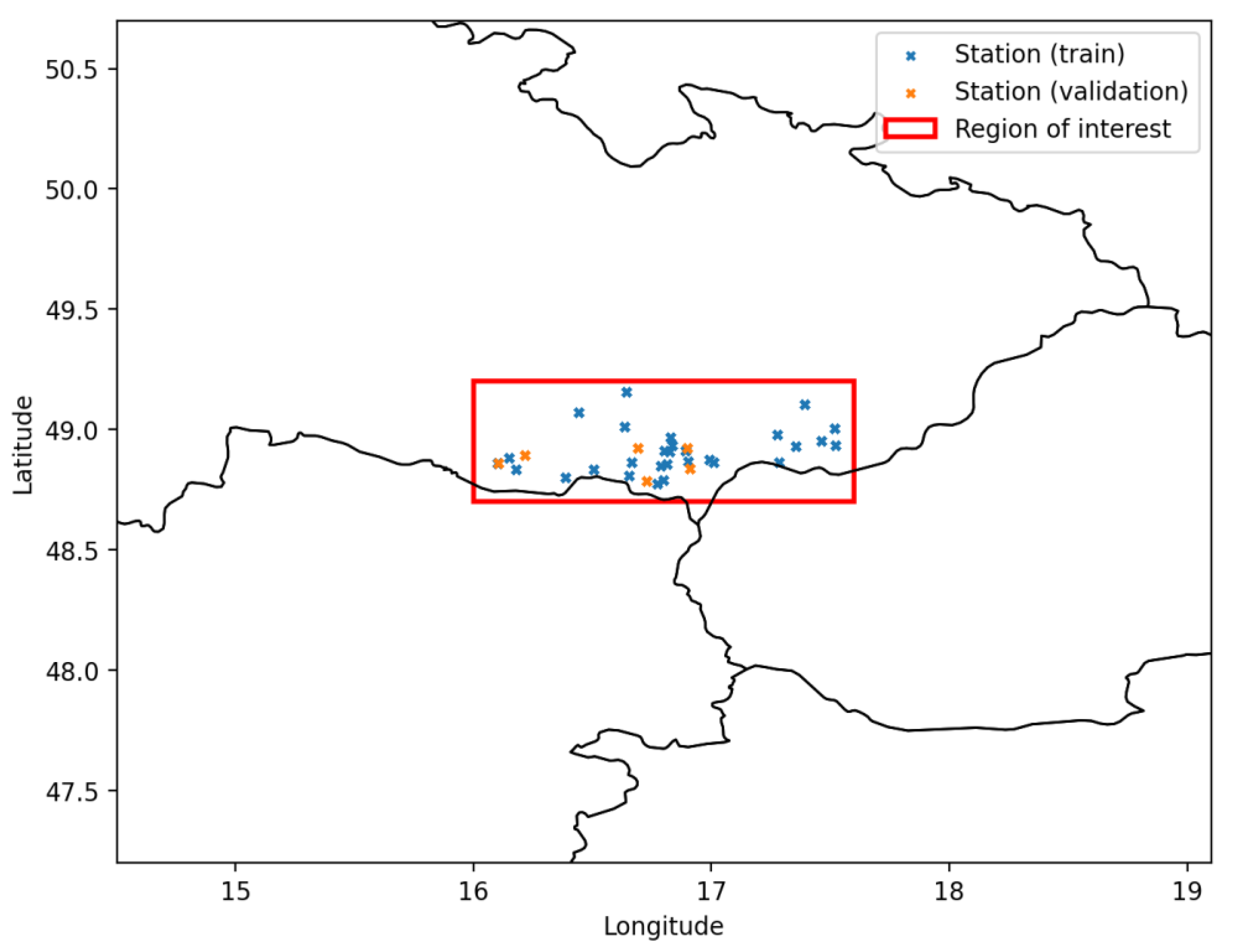
Figure 3.
Mean absolute error (MAE) of predicted temperature 24 hours ahead for each possible space and time split for each model.
Figure 3.
Mean absolute error (MAE) of predicted temperature 24 hours ahead for each possible space and time split for each model.
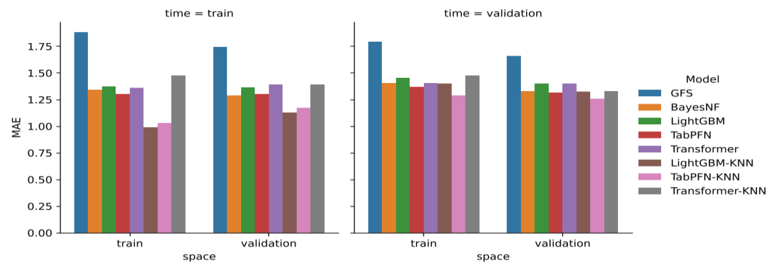
Figure 4.
Example of predicted temperature of all models and the target temperature over a time period for each weather station in the validation split.
Figure 4.
Example of predicted temperature of all models and the target temperature over a time period for each weather station in the validation split.
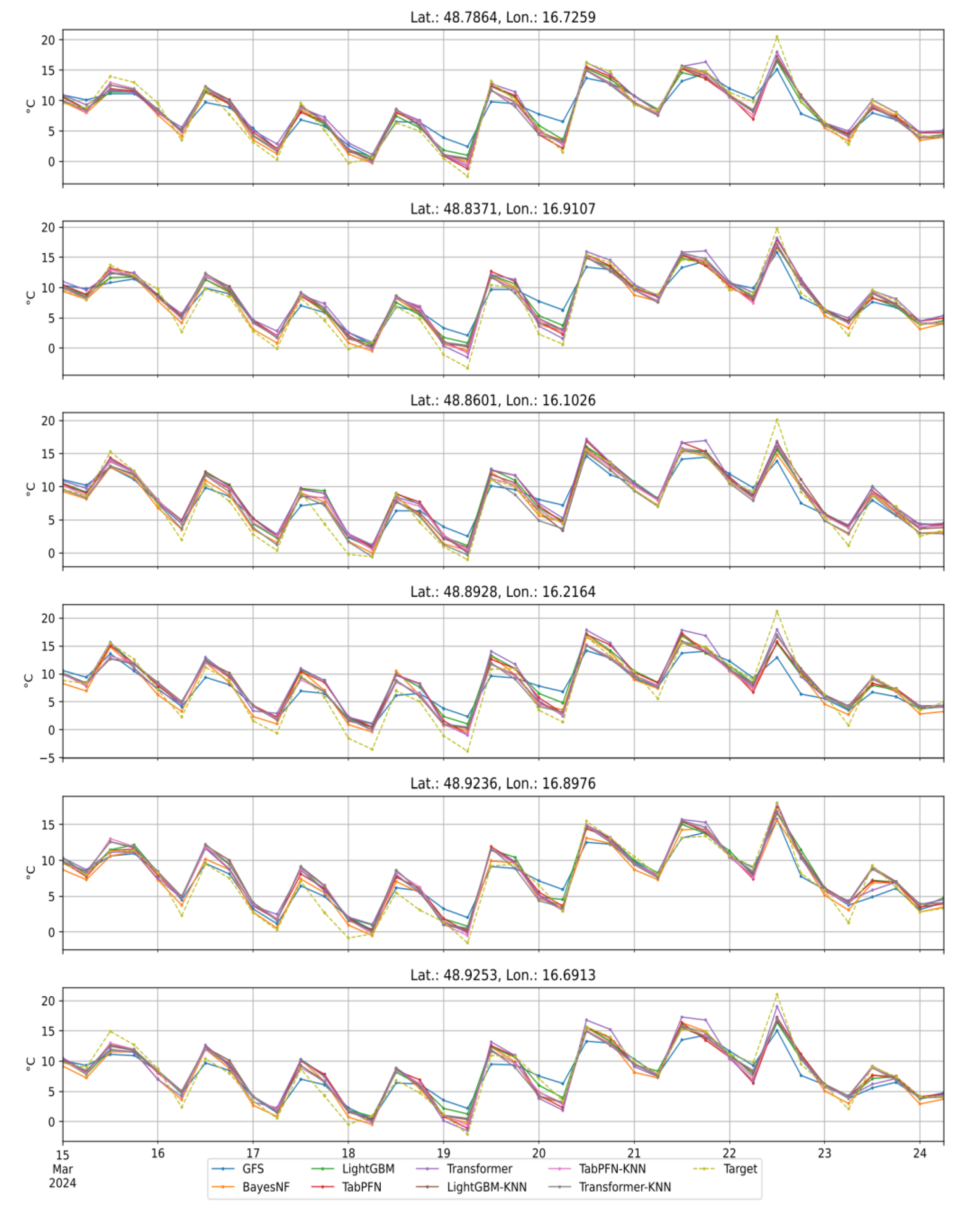
Figure 5.
Example of predicted temperature 24 hours ahead for all models on the selected region (case A).
Figure 5.
Example of predicted temperature 24 hours ahead for all models on the selected region (case A).
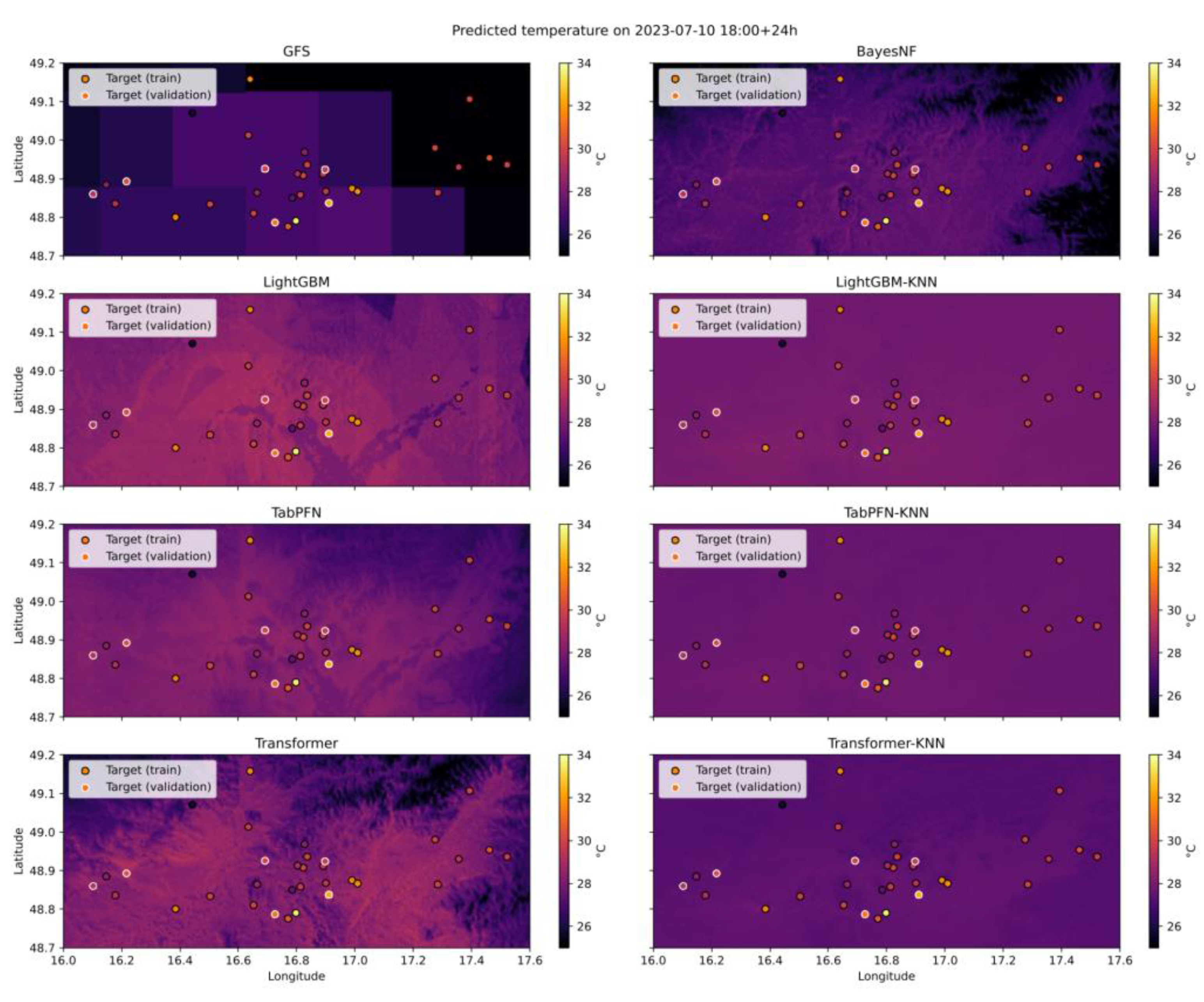
Figure 6.
Example of predicted temperature 24 hours ahead for all models on the selected region (case B).
Figure 6.
Example of predicted temperature 24 hours ahead for all models on the selected region (case B).
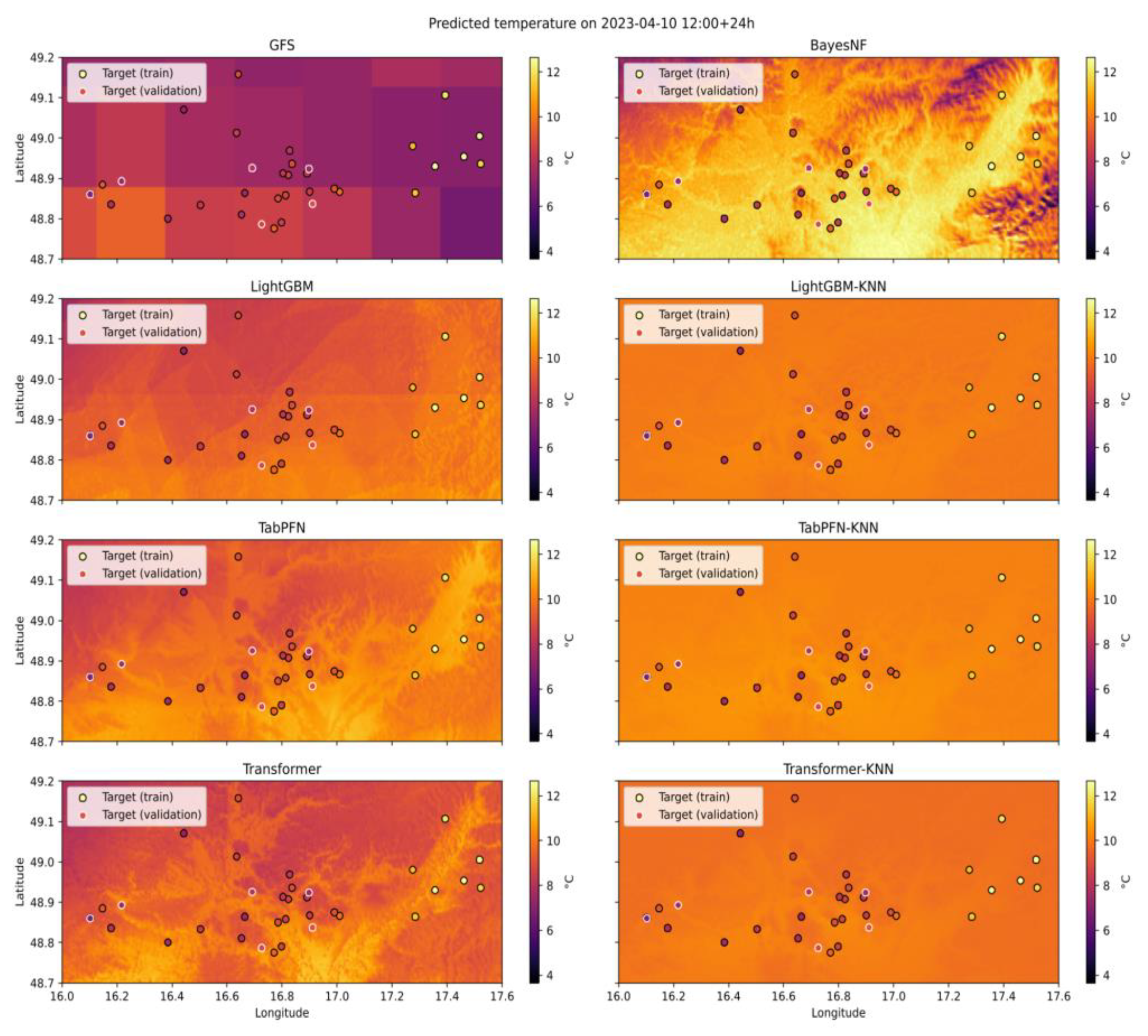

Table 1.
Mean absolute error (MAE) of predicted temperature 24 hours ahead for each possible space and time split for each model.
Table 1.
Mean absolute error (MAE) of predicted temperature 24 hours ahead for each possible space and time split for each model.
| Model | Time=train, Space=train | Time=train, Space=validation | Time=validation, Space=train | Time=validation, Space=validation |
|---|---|---|---|---|
| GFS | 1.88 | 1.75 | 1.79 | 1.66 |
| BayesNF | 1.34 | 1.29 | 1.40 | 1.33 |
| LightGBM | 1.37 | 1.37 | 1.46 | 1.40 |
| TabPFN | 1.30 | 1.30 | 1.37 | 1.32 |
| Transformer | 1.36 | 1.39 | 1.40 | 1.40 |
| LightGBM–KNN | 0.99 | 1.13 | 1.40 | 1.32 |
| TabPFN–KNN | 1.03 | 1.17 | 1.29 | 1.26 |
| Transformer–KNN | 1.48 | 1.39 | 1.48 | 1.33 |
Disclaimer/Publisher’s Note: The statements, opinions and data contained in all publications are solely those of the individual author(s) and contributor(s) and not of MDPI and/or the editor(s). MDPI and/or the editor(s) disclaim responsibility for any injury to people or property resulting from any ideas, methods, instructions or products referred to in the content. |
© 2025 by the authors. Licensee MDPI, Basel, Switzerland. This article is an open access article distributed under the terms and conditions of the Creative Commons Attribution (CC BY) license (http://creativecommons.org/licenses/by/4.0/).
Copyright: This open access article is published under a Creative Commons CC BY 4.0 license, which permit the free download, distribution, and reuse, provided that the author and preprint are cited in any reuse.


