
Submitted:
18 December 2025
Posted:
22 December 2025
You are already at the latest version
Abstract
Prostate cancer is one of the most lethal cancers in the male population, and accurate localization of intraprostatic lesions on MRI remains challenging. In this work, we investigate methods for improving prostate cancer segmentation on T2weighted pelvic MRI using cascaded neural networks. We use anonymized dataset of 400 multiparametric MRI studies from two centers, in which experienced radiologists delineated the prostate and clinically significant cancer on the T2 series. Our baseline approach applies 2D and 3D segmentation networks (UNETR, UNET++, SwinUNETR, SegResNetDS, SegResNetVAE) directly to full MRI volumes. We then introduce additional stages that filter slices using DenseNet201 classifiers (cancer/nocancer and prostate/noprostate) and localize the prostate with a YOLObased detector to crop a 3D region of interest before segmentation. Using SwinUNETR as the backbone, the prostate segmentation Dice score increased from 71.37% for direct 3D segmentation to 76.09% when using prostate detection and cropped 3D inputs. For cancer segmentation, the final cascaded pipeline – prostate detection, 3D prostate segmentation, and 3D cancer segmentation within the prostate – improved Dice score from 55.03% for direct 3D segmentation to 67.11%, with a ROC AUC of 0.89 on the test set. These results suggest that cascaded detection and segmentationbased preprocessing of the prostate region can substantially improve automatic prostate cancer segmentation on MRI while remaining compatible with standard segmentation architectures.
Keywords:
prostate cancer
; prostate MRI
; deep learning
; semantic segmentation
; artificial intelligence
; biomedical image analysis
1. Introduction
Prostate cancer is one of the leading causes of cancer-related deaths in men [1]. One of the reasons for this high mortality is the difficulty in diagnosing the disease in its early stages. The classic method for detecting cancer is Prostate Specific Antigen (PSA) monitoring. If its level increases, the patient is referred for additional testing, including a multiparametric MRI. mpMRI is performed in various modes and sent to a radiologist for analysis. A special PI-RADS scale has been developed for MRI-based cancer diagnosis. This scale is used by specialists to verify detected changes in the prostate gland and determine their clinical significance [2].
When prostate cancer is detected in the late stages, MRI is used to plan surgical interventions. There are advanced developments in the use of artificial intelligence software for surgical planning. For example, AI can be used for 3D reconstruction of the prostate and the use of these data in planning tumor-removal surgery [3,4]. However, detecting cancer in the early stages is difficult because healthy and diseased tissues often have poor contrast.
When considering the application of AI in medicine in general, it is worth mentioning that during the COVID-19 pandemic, many studies were conducted on the use of AI to solve classification and segmentation problems [5,6]. In particular, the main emphasis in the analysis of lung diseases was placed on the analysis of CT studies and radiographs. Among the systems for analyzing CT scans of the lungs, the work of Jin, C., Chen, W., Cao, Y. et al. [7] is noteworthy. They obtained ROC AUC > 0.90 in the analysis of CT studies for lung damage from COVID-19 and pneumonia (viral and non-viral) and also used visualization of the locations to which the neural network responded using grad-cam [8].
Among all the problems in medicine that utilize AI, three fundamental image processing tasks are the most widely used: classification, detection, and segmentation. A classification model assumes the presence of an object that must be assigned to one of the established classes. A prime example of this is the detection of pathology, such as broken ribs in CT scans [9,10] or the work during the pandemic [11].
The detection task is to locate an object of a specified class in an image and construct a frame containing the object. In medicine, detection algorithms are used when it is necessary to precisely localize a detected object. Information about the object's localization potentially allows not only to establish the object's presence but also to obtain more precise data, such as assigning a broken rib to the right or left side of the body [10]. The use of detection has also been explored in detecting gastric cancer in endoscopic images [12].
Segmentation allows for pixel-by-pixel division of an image into classes. In medicine, neural networks for segmentation are primarily used to identify pathologies (for example, brain pathologies) or to identify organ boundaries in CT or MRI scans [13,14].
For most solutions, a single neural network architecture specific to the problem domain is sufficient. However, solving complex problems may require integrated approaches, including the use of multiple neural networks, including networks for specific tasks, such as image registration [15].
Our work aims to identify and describe an optimal method for segmenting prostate cancer on pelvic MRI. The primary objective is to segment the prostate and the cancer within its boundaries. The study used anonymized data from a dataset containing 400 studies. The data was collected at two medical institutions: the Mariinsky Hospital and the Petrov Research Institute. In all MRI studies, specialists with over 10 years of radiology experience mapped the prostate and the cancer.
Among the studies related to ours, we can highlight the study [14], in which a group of researchers used a two-stage approach for cancer segmentation. Wei C. et al., in their study, used a neural network to solve the problem of prostate segmentation (first stage) and cancer segmentation in a refined region of the prostate (second stage). The authors show that the use of a two-stage approach allows improving the results of cancer segmentation by 0.07 for U-Net and 0.18 for attention U-Net, relative to a one-stage approach, when cancer segmentation is performed without preliminary selection of the prostate region. Another example is the study [16] in which the authors used a combination of three parametric series of multi-parametric MRI as data. During the study, they obtained results comparable to an experienced person. Another study that evaluated the capabilities of trained models and compared their results with those of experienced specialists is [17], in which the authors compared the quality of prostate cancer detection of neural networks trained on more than 10,000 MRI studies collected from different locations and different devices, with the results of the work of experienced diagnostic doctors. The results indicate that, with enough data for training, trained neural networks can show results close to the quality of the work of specialists. In addition to the cited works, it is worth noting that [18] emphasizes the relevance of this research direction and the trend toward translating AI from abstract research into commercial medical applications.
In biomedical image analysis, clean masks of the prostate and intraprostatic cancer on MRI are a basic step that many clinical tools rely on. We treat this as an algorithm design problem and use a small, modular cascade: first detect the prostate, then segment the gland, and then segment cancer inside it. By focusing the models on a tight region of interest, the pipeline reduces background noise and false positives, gives more stable results across scanners and sites, and outputs masks that are easy for clinicians to check and reuse.
2. Materials and Methods
2.1. Image Segmentation
Semantic segmentation is an important approach when working with medical images, including problems of delineating individual organs or tumors. The essence of this method is to assign each pixel based on the context of the pixel relative to its environment. Currently, there are many variations of neural network architectures for segmenting medical images, ranging from the classic U-Net network with a U-shaped structure of the encoder and decoder at the core to the integration of Transformers for image processing - SWINUnet, which also has a self-attention mechanism. However, it is worth noting that with the transition from 2D medical image analysis to multi-series data (such as CT and MRI), implementations of architectures for full-fledged analysis of 3D data have appeared. This means creating architectures that can capture context not only within a 2D slice but also across the 3D image volume, which allows for a more accurate determination of the boundaries of organs or tumor inclusions since the spatial relationship between the slices is considered [19,20,21,22,23,24,25,26,27,28,29].
In our study, we used two segmentation settings. In the first, we split 3D MRI data into separate slices and passed them to a network for 2D slice segmentation. UNETR, UNET++, and Swin-UNETR are investigated as neural networks for segmentation. In the second case, training is carried out on loaded 3D data for the segmentation of MRI as a whole. The following architectures are used as trained networks: Swin-UNETR, UNETR, SegResNetDS, SegResNetVAE.
The main metric for segmentation models was the calculation of the Dice-Sorensen (Dice) coefficient. This coefficient quantifies the overlap between two areas. For the task of 2D segmentation, the coefficient is calculated between the true mask of the object (ground truth) and the neural network's prediction (Eq. 1). When implementing the metric in 3D segmentation, additional summation is introduced over all slices with at least one of the masks, and the average coefficient for a series of images is calculated (Eq. 2).
where X and are the predicted mask for 2D segmentation and the i-th predicted mask for 3D segmentation, Y and are the true mask for 2D segmentation, and the i-th true mask for 3D segmentation, n is the number of 3D image slices that contain at least one mask. An example of calculating the metric is shown in Figure 1 below.
2.2. Image Detection
Object detection in an image involves determining the location of an object of a given class if it is present in the image. The location of an object is determined by enclosing the object in certain boundaries, most often in a bounding box. Detection is often applied to medical problems to highlight an area of interest in the context of various tasks, for example, an area containing an organ or a tumor. The development of detection architectures has progressed from basic convolutional networks, such as R-CNN, to more complex ones, such as YOLO in its various versions [30,31]. An example of determining the prostate area in an image is shown in Figure 2.
Our work relied on YOLOv9 to solve the detection problem. A built-in validation set was used to assess the quality of the trained model, including the mAP50–95 metric. This metric shows the area under the Precision-Recall curve for threshold 0.5, 0.95.
2.3. Image Classification
Classification assigns objects to predefined classes. In medicine, neural classification networks are typically used to identify images with pathologies (for example, whether there is a pathology on an X-ray or not) or as a routing step (for example, to determine which part of the body an X-ray image belongs to before sending it to the appropriate analysis service). A full history is beyond the scope of this paper [32,33,34,35,36,37,38,39]. However, fully connected and convolutional neural networks laid down the basic principles, which later grew into such architectures as ResNet and DenseNet, Transformer.
To assess the quality of the model, standard metrics were used (the list is given in the next paragraph), as well as the Area Under the Receiver Operating Characteristic Curve (ROC AUC) metric. This metric is constructed in the coordinates of sensitivity and 1 - specificity, with different thresholds for classifying an object into a target class. This metric clearly shows how accurately the model performs classification. It is worth noting that the ROC AUC metric can also be used to evaluate segmentation models. To do this, you need to set the Dice metric threshold at which segmentation is considered successful and belongs to class 1, and everything below the threshold is classified as class 0. In this case, the ROC curve thresholds relate to the activation threshold for image pixels. In our experiments, a Dice score of 0.5 was chosen as the threshold for successful segmentation.
2.4. Additional Metrics
To comprehensively assess the quality of the trained segmentation models, the study used additional metrics listed in the table below. When calculating the metrics, a threshold of Dice ≥ 0.5 was set to classify the segmentation as “correct segmentation”, which corresponded to “1”.

Table 1.
Description of the metrics used.
| Metric | Description |
| Accuracy | Shows the overall correctness of the segmentation |
| Precision | Shows the proportion of positive pixels relative to all pixels classified as positive |
| Recall | Shows the proportion of positive pixels relative to all true positive pixels |
| Specificity |
Shows the ability to identify negative pixels correctly |
| F1 | based on precision and recall, and displays a balanced measure of segmentation accuracy |
2.5. Dataset
As a dataset for training the networks and assessing the quality of the results obtained, we used a closed dataset collected from two hospitals:
- Mariinsky Hospital - 183 MRI studies of the pelvis.
- Petrov Research Institute - 217 MRI studies of the pelvis
In total, the dataset contained 400 anonymized pelvic mpMRI studies from men aged 25–62 years. Each of the studies was reviewed by three specialists who identified signs of clinically significant prostate cancer of different stages. Also, each T2 series of studies from the dataset was marked by radiologists to highlight the prostate area and prostate cancer.
We used the T2 series of each study to train neural networks since they are the clearest and most easily interpreted by humans and are most suitable for analysis by neural network algorithms.
The division of all data into training, validation, and test sets was performed using the built-in tools of the MONAI framework with a fixed random seed in the following ratios:
- for segmentation (2D and 3D): train - 0.7, val - 0.2, test - 0.1;
- for detection: train - 0.85, test - 0.15;
- for classification: train - 0.7, val - 0.2, test - 0.1.
All splits were performed at the study level, such that all slices from a given mpMRI examination were assigned to the same set (train, validation, or test) for every task.
2.6. Hardware and Software Setup
2.7. Method
Our main goal is to obtain accurate segmentation of prostate cancer. However, during the study, we encountered the fact that simply using a neural network for cancer segmentation did not produce acceptable results on our dataset, so we began searching for methods to improve prostate cancer segmentation. Based on the progress of the entire study and the results obtained, we can divide the research process into three stages: preliminary, main, and final.
During the preliminary stage, we used neural networks for prostate cancer segmentation, as well as an approach that preliminarily utilized a classifier trained to separate sections into two classes: "with cancer" and "without cancer." In the first case, we employed two approaches to cancer segmentation: segmentation of 2D data and segmentation of 3D data. In the second case, we first created a new dataset, retaining only those sections labeled by the classifier as containing cancer. The new dataset was then used to train neural networks for 2D and 3D segmentation. A schematic of the final algorithm, using a single study from this stage as an example, is shown in Figure 3.
To improve the results of the preliminary stage, we decided to use only the prostate region for cancer segmentation. This required us to extract only the prostate region and then train the model on the new data. The main phase of our study was based on prostate-region extraction and consisted of three stages. In the first stage, we used neural segmentation networks to extract the prostate from 2D and 3D data from entire studies, without first creating a new dataset.
To improve the results, we decided to try the idea from the preliminary stage: only feeding slices containing the prostate to the segmentation networks. To do this, we trained a neural network for binary classification (presence/absence of the prostate in the slice). We then created a new dataset. However, at this stage, we modified the rule for creating the new dataset: we now included only slices in the range from the lowest to the highest slice number. This approach is justified by the fact that the prostate is a continuous organ, thus eliminating possible classifier error in the midsection. The new dataset was split according to the proportions specified in 2.6 and used for 2D and 3D segmentation. A schematic representation of the algorithm using a single series as an example is shown in Figure 4.
Since some segmentation errors were found among the segmentation results, we decided to further refine the target region and use a neural network for detection as a preprocessing step. This network detected the prostate and enclosed it in a bounding box. To avoid cropping out part of the prostate (if the detection was inaccurate) and to ensure uniform data size (across the study), we calculated the maximum coordinates among all frames (maximum height and width) and increased them by 5% in each direction.
We then cropped the studies, thereby creating a parallelepiped smaller than the original MRI study but containing the target region with the prostate. Segmentation training was also performed on the new dataset. A schematic representation of the algorithm using a single series as an example is shown in Figure 5.
The final stage involved using the best prostate segmentation method to generate a modified dataset containing only the prostate region and training a cancer segmentation network with the best performance from the preliminary stage. A schematic representation of the entire final stage algorithm is shown in Figure 6.
3. Experiments
3.1. Preliminary Stage. Training 2D and 3D Cancer Segmentation Networks
At this stage, we trained neural networks for 2D cancer segmentation. The training dataset consisted of MRI scans. Three architectures were chosen as training neural networks: UNETR, UNET++, Swin-UNETR. The configuration parameters of the neural networks used, the training configuration, the metric used, and the error function for this and all other neural networks are presented in Tables S1 and S2.
To train neural networks for segmentation on 3D data (entire MRI scans), we chose four architectures: UNETR, Swin-UNETR, SegResNetDS, and SegResNetVAE. The training configurations and training graphs are presented below.
At this stage, we also trained the classification network. DenseNet-201 was chosen as the training architecture. After training DenseNet-201 (Figure 7 and Figure 8), we created a modified dataset for 2D and 3D segmentations. For the 2D data, it consisted of slices from MRI scans that the classification network classified as prostate cancer. For the 3D dataset, we created "stripped" MRI scans, which included only those slices labeled as prostate cancer, as well as one slice before and one slice after the classified sequence. This expansion was used to reduce the risk of classifier error.
Since the 2D dataset contained less data after the classifier, but the data itself remained unchanged, we did not retrain the classification networks; we only tested them on the new dataset. However, the networks for 3D segmentation were retrained because the data in the dataset had essentially changed (the number of slices, and therefore the third dimension in the transmitted tensor, had changed). The same set of networks was used for retraining. The configurations and training process are presented below.
3.2. Main Stage. Training 2D and 3D Prostate Segmentation Networks
To train networks for prostate segmentation, we decided to use the same architecture as in the preliminary stage. Prostate masks were used as data. The training dataset and the training process itself were prepared in a similar manner.
To train prostate segmentation on entire MRI studies (3D data), we also selected the architectures used for 3D prostate cancer segmentation. The training dataset and the training process itself were prepared in a similar manner.
The next step at this stage was to replicate the experience of using a classifier to restrict uninformative slices for segmentation. As in the preliminary stage, the DenseNet-201 neural network was chosen as the classifier. The configuration and training parameters are presented in Table S3.
After training the classifier, we updated the datasets for training 2D and 3D segmentations. The generation rule for the updated datasets was almost identical to the generation rule described in the preliminary stage, except that slices ranging from the minimum slice number classified as prostate to the maximum slice number were used to generate the new 3D data. This approach was adopted from the anatomy of the prostate: it is a continuous organ that is not divided into two or more parts, unlike cancer lesions, which can be multiple in different areas of the prostate gland.
Since the tasks of segmenting prostate cancer and prostate are essentially identical, we again faced the need to retrain the 3D segmentation networks, as the new 3D data was smaller than the original. The network configuration and training process are presented below. We achieved a slight improvement in the main Dice metric, as using the classifier required feeding the network fewer slices, resulting in fewer false positives. Our next step was to use detection instead of classification, as this would minimize the number of unnecessary inclusions and structures in the data passed to segmentation.
As a working approach, we developed the following algorithm: submitting the MRI scan for detection, obtaining bounding box coordinates, finding the maximum coordinates (for each of the four box vertices), incrementing each by 5%, rounding up, and cropping the original MRI scan to the resulting parallelepiped. In this approach, increasing the frame size (by 5% on each side) is necessary to avoid possible random errors in detection. Next, we needed to resize all the obtained data to a uniform size, since the resulting frames were smaller than the original image in any case. The standard image size was chosen to be 128 x 128 x 24 (in the case of 3D data), and resizing was done using PyTorch tools.
The popular and powerful YOLO architecture was used to train the detection network. The training parameters and standard set of post-training metrics are listed below in Table 3 and Figure 9.
Two architectures were chosen as trainable neural networks for working with 2D slices: UNET++ and Swin-UNETR. For training on entire MRI studies, we chose Swin-UNETR and SegResNetDS.
Among all the trained neural networks for segmentation, the Swin-UNETR architecture demonstrated the best results at the preliminary and main stages. Plots for the Dice metric, as well as plots for the error function, are presented below: for 2D segmentation in Figure 10 and Figure 11, respectively, and for 3D segmentation in Figure 12 and Figure 13.
3.3. Final Stage. Dataset Formation and Segmentation Training
The final stage consisted of preparing the dataset and training the neural network for cancer segmentation using new data. To generate the dataset, we used the best method from the main stage, namely, a combination of preliminary detection and subsequent 3D segmentation using the Swin-UNETR network. For training, we selected the architecture with the best 2D and 3D cancer segmentation performance from the preliminary stage—this was also the Swin-UNETR architecture in both cases. The training process is presented below.
Figure 14.
Graphs of Dice changes during the training of the Swin-UNETR network at the final stage (a) Dice change from epoch to epoch on the training set; (b) Dice change from epoch to epoch on the validation set.
Figure 14.
Graphs of Dice changes during the training of the Swin-UNETR network at the final stage (a) Dice change from epoch to epoch on the training set; (b) Dice change from epoch to epoch on the validation set.
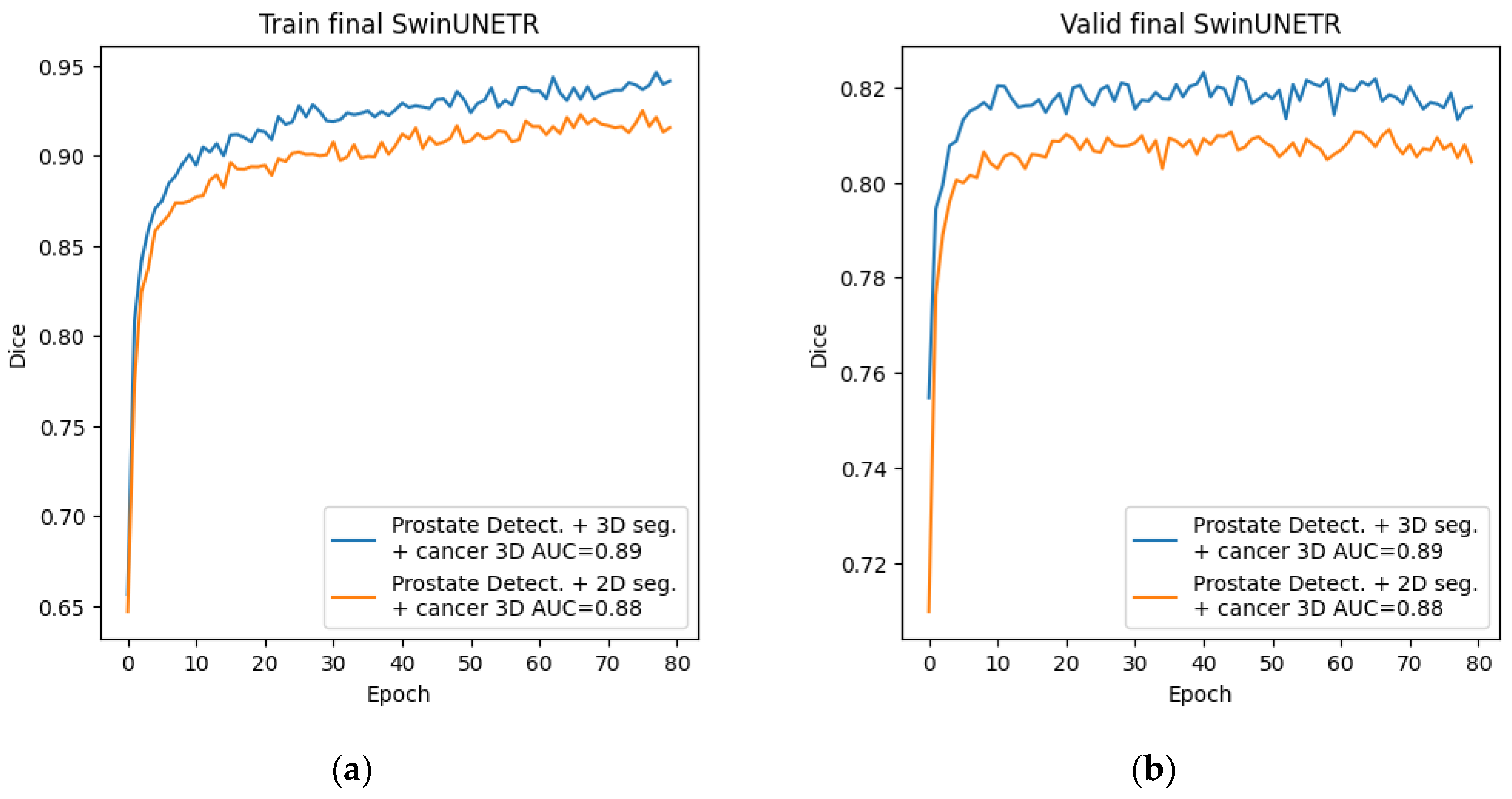
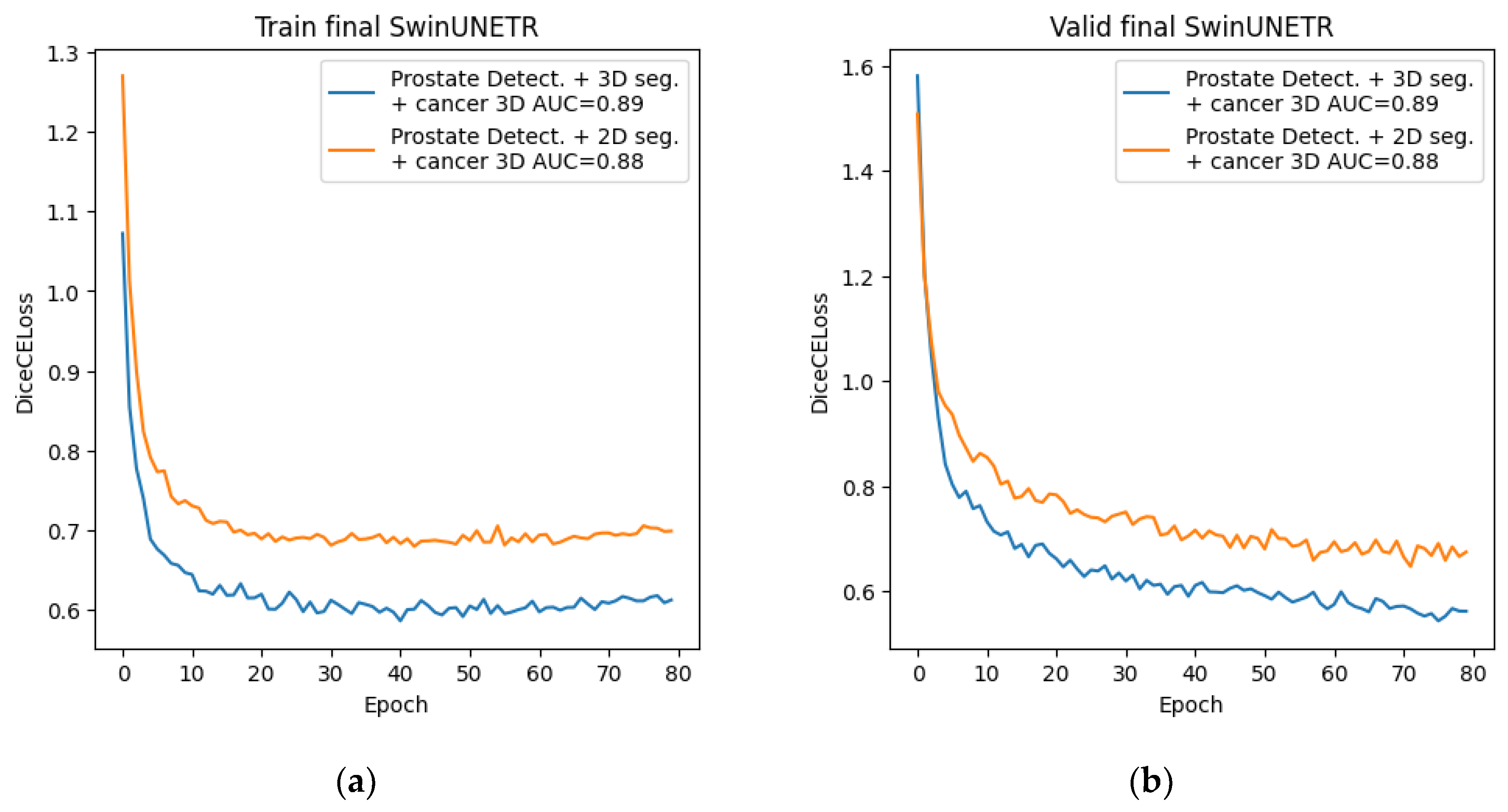
Figure 15.
Graphs of Dice changes during Swin-UNETR network training at the final stage: (a) Dice change from epoch to epoch on the training set; (b) Dice change from epoch to epoch on the validation set.
Figure 15.
Graphs of Dice changes during Swin-UNETR network training at the final stage: (a) Dice change from epoch to epoch on the training set; (b) Dice change from epoch to epoch on the validation set.
4. Results
In this study, the best prostate cancer segmentation performance was achieved with the final-stage pipeline using 3D cancer segmentation. ROC AUC plots (Figure 16) for the trained segmentation models used in the final stage are presented below.
An example of segmentation of cancer foci by the final 2D cancer segmentation model is shown in Figure 17.
An example of segmentation of cancer foci by the final 3D cancer segmentation model is shown in Figure 18.
A summary of all metrics for each trained segmentation network is provided in Table 4. It does not include data for the classifier metrics or the YOLO detection network, as these networks were trained as a single instance for their task.
5. Discussion
In this paper, we explored methods for improving prostate cancer segmentation results. Although using cancer classification on a slice for further segmentation did not yield significant improvements, this prompted the idea of using the prostate region for cancer segmentation. This approach led to an analysis of conventional prostate segmentation and two ways to improve it: classification and detection. The results show that using detection to isolate the prostate region can increase the accuracy of organ segmentation, which can conceptually be transferred to other applied segmentation tasks.
A potential bottleneck of this approach to segmentation is the loss of algorithmic flexibility in dealing with variable data. During our study, we encountered 8 MRI studies that had significant deviations in contrast values relative to the rest of the dataset. These studies had the worst prostate and cancer segmentation results, even though prostate detection did not materially affect bounding-box localization. One of the future directions of our research will be to find methods to address this issue.
Another issue we encountered, which prompted us to use prostate segmentation for data improvement, was the problem of abrupt data changes when using the classifier. This problem arose when two cancer lesions had sections of healthy prostate tissue between them. With such lesions, when generating a modified dataset after the cancer classifier, sharp boundaries appeared within the segmented data, which was especially noticeable in 3D segmentation. In our work, we avoided this problem by using the prostate region as the transferred data, but it may arise in other segmentation applications using modified datasets.
Beyond technical performance, the proposed pipeline has several potential clinical applications. Robust prostate and cancer segmentation on MRI could support personalized care by assisting radiologists in lesion localization, enabling more precise targeting of biopsies and focal treatments, and providing quantitative tumor volumes for risk stratification and treatment response assessment at the individual-patient level. In radiotherapy, accurate organ and tumor masks are also essential for automated contouring and dose planning; improving segmentation quality may therefore translate into more consistent, patient-specific treatment plans. Prospective studies will be needed to confirm these benefits in real-world clinical workflows.
6. Conclusions
In this study, we explored a cascaded approach to improve prostate cancer segmentation on T2-weighted pelvic MRI. Starting from direct 2D and 3D segmentation of cancer, we incrementally refined the input data by incorporating prostate-focused preprocessing steps: slice-level classification, YOLO-based prostate detection, and 3D prostate segmentation. On a dataset of 400 annotated MRI studies from two clinical centers, the best prostate segmentation performance was obtained with a combination of prostate detection and 3D Swin-UNETR segmentation (Dice 76.09%). Using this refined prostate region as input for 3D cancer segmentation increased the cancer Dice coefficient from 55.03% for direct 3D Swin-UNETR segmentation to 67.11%, with a ROC AUC of 0.89, demonstrating that isolating the prostate region meaningfully improves cancer segmentation quality.
At the same time, the proposed solution increases pipeline complexity, as it relies on several sequential networks for classification, detection, and segmentation. The approach may be sensitive to variations in image acquisition: in our dataset, a small subset of studies with markedly different contrast characteristics showed the poorest segmentation performance despite accurate detection, highlighting robustness as an important limitation. Future work will focus on handling such heterogeneous studies, assessing generalization on additional external cohorts, and investigating whether the cascaded strategy can be simplified or adapted to multi-parametric inputs while preserving or further improving prostate and cancer segmentation accuracy.
Supplementary Materials
The following supporting information can be downloaded at the website of this paper posted on Preprints.org, Table S1: The parameters of configuration each segmentation neural network, Table S2: Optimizer and training parameters, Table S3: Configuration and training parameters for the classification networks.
Author Contributions
Conceptualization, N.N. and N.S.; methodology, N.N.; software, N.S.; validation, R.D., N.N. and N.S.; formal analysis, N.S.; investigation, N.N.; resources, N.N.; data curation, N.N.; writing—original draft preparation, N.N. and R.D.; writing—review and editing, N.N. and R.D.; visualization, N.N.; supervision, N.S. and R.D; project administration, N.S.; funding acquisition, R.D. All authors have read and agreed to the published version of the manuscript.
Funding
This research received no external funding.
Informed Consent Statement
Not applicable.
Data Availability Statement
The data presented in this study are available on request from the corresponding author.
Conflicts of Interest
The authors declare no conflicts of interest.
References
- Sung, H.; Ferlay, J.; Siegel, R.L.; Laversanne, M.; Soerjomataram, I.; Jemal, A.; Bray, F. Global cancer statistics 2020: GLOBOCAN estimates of incidence and mortality worldwide for 36 cancers in 185 countries. CA Cancer J. Clin. 2021, 71, 209–249. [Google Scholar] [CrossRef] [PubMed]
- Turkbey, B.; Rosenkrantz, A.B.; Haider, M.A.; Padhani, A.R.; Villeirs, G.; Macura, K.J.; Tempany, C.M.; Choyke, P.L.; Cornud, F.; Margolis, D.J.; Thoeny, H.C.; Verma, S.; Barentsz, J.; Weinreb, J.C. Prostate Imaging Reporting and Data System Version 2.1: 2019 update of Prostate Imaging Reporting and Data System Version 2. Eur. Urol. 2019, 76, 340–351. [Google Scholar] [CrossRef]
- Cianflone, F.; Maris, B.; Bertolo, R.; Veccia, A.; Artoni, F.; Pettenuzzo, G.; Montanaro, F.; Porcaro, A.B.; Bianchi, A.; Malandra, S.; Ditonno, F.; Cerruto, M.A.; Zamboni, G.; Fiorini, P.; Antonelli, A. Development of artificial intelligence-based real-time automatic fusion of multiparametric magnetic resonance imaging and transrectal ultrasonography of the prostate. Urology 2025, 199, 27–34. [Google Scholar] [CrossRef] [PubMed]
- Palazzo, G.; Mangili, P.; Deantoni, C.; Fodor, A.; Broggi, S.; Castriconi, R.; Ubeira Gabellini, M.G.; Del Vecchio, A.; Di Muzio, N.G.; Fiorino, C. Real-world validation of artificial intelligence-based computed tomography auto-contouring for prostate cancer radiotherapy planning. Phys. Imaging Radiat. Oncol. 2023, 28, 100501. [Google Scholar] [CrossRef] [PubMed]
- Sheng, K. Artificial intelligence in radiotherapy: A technological review. Front. Med. 2020, 14, 431–449. [Google Scholar] [CrossRef]
- Francolini, G.; Desideri, I. Artificial intelligence in radiotherapy: State of the art and future directions. Med. Oncol. 2020, 37, 50. [Google Scholar] [CrossRef]
- Jin, C.; Chen, W.; Cao, Y.; et al. Development and evaluation of an artificial intelligence system for COVID-19 diagnosis. Nat. Commun. 2020, 11, 5088. [Google Scholar] [CrossRef]
- Selvaraju, R.R.; Cogswell, M.; Das, A.; Vedantam, R.; Parikh, D.; Batra, D. Grad-CAM: Visual explanations from deep networks via gradient-based localization. In Proceedings of the IEEE International Conference on Computer Vision (ICCV), 2017 ; pp. 618–626. [Google Scholar] [CrossRef]
- Zhou, Q.-Q.; Hu, Z.-C.; Tang, W.; et al. Precise anatomical localization and classification of rib fractures on CT using a convolutional neural network. Clin. Imaging 2022, 81, 24–32. [Google Scholar] [CrossRef]
- Zhou, Q.-Q.; Wang, J.; Tang, W.; Hu, Z.-C.; Xia, Z.-Y.; Li, X.-S.; Zhang, R.; Yin, X.; Zhang, B.; Zhang, H. Automatic detection and classification of rib fractures on thoracic CT using convolutional neural network: Accuracy and feasibility. Korean J. Radiol. 2020, 21, 869–879. [Google Scholar] [CrossRef]
- Aggarwal, P.; Mishra, N. COVID-19 image classification using deep learning: Advances, challenges and opportunities. Comput. Biol. Med. 2022, 144, 105350. [Google Scholar] [CrossRef]
- Hirasawa, T.; Aoyama, K.; Tanimoto, T.; et al. Application of artificial intelligence using a convolutional neural network for detecting gastric cancer in endoscopic images. Gastric Cancer 2018, 21, 653–660. [Google Scholar] [CrossRef]
- Ghaffari, M.; Sowmya, A. Automated brain tumor segmentation using multimodal brain scans: A survey based on models submitted to the BraTS 2012–2018 challenges. IEEE Rev. Biomed. Eng. 2020, 13, 156–168. [Google Scholar] [CrossRef]
- Wei, C.; Liu, Z.; Zhang, Y.; Fan, L. Enhancing prostate cancer segmentation in bpMRI: Integrating zonal awareness into attention-guided U-Net. Digital Health 2025, 11. [Google Scholar] [CrossRef]
- Nefediev, N.A.; Staroverov, N.E.; Davydov, R.V. Improving compliance of brain MRI studies with the atlas using a modified TransMorph neural network. St. Petersburg State Polytechnical University Journal. Physics and Mathematics 2024, 17(3.1), 335–339. [Google Scholar] [CrossRef]
- Mehrtash, A.; Sedghi, A.; et al. Classification of clinical significance of MRI prostate findings using 3D convolutional neural networks. Proc. SPIE 2017, 10134, 101342A. [Google Scholar] [CrossRef]
- Saha, A.; Bosma, J.S.; Twilt, J.J.; PI-CAI Consortium. Artificial intelligence and radiologists in prostate cancer detection on MRI (PI-CAI): An international, paired, non-inferiority, confirmatory study. Lancet Oncol. 2024, 25, 879–887. [Google Scholar] [CrossRef] [PubMed]
- Ng, C.K.C. Performance of commercial deep learning-based auto-segmentation software for prostate cancer radiation therapy planning: A systematic review. Information 2025, 16, 215. [Google Scholar] [CrossRef]
- Gaziev, G.; Wadhwa, K.; Barrett, T.; Koo, B.C.; Gallagher, F.A.; Serrao, E.; Frey, J.; Seidenader, J.; Carmona, L.; Warren, A.; Gnanapragasam, V.; Doble, A.; Kastner, C. Defining the learning curve for multiparametric magnetic resonance imaging (MRI) of the prostate using MRI–transrectal ultrasonography (TRUS) fusion-guided transperineal prostate biopsies as a validation tool. BJU Int. 2016, 117, 80–86. [Google Scholar] [CrossRef]
- Myronenko, A. 3D MRI brain tumor segmentation using autoencoder regularization. In Brainlesion: Glioma, Multiple Sclerosis, Stroke and Traumatic Brain Injuries; 4th International Workshop, BrainLes 2018;Revised Selected Papers, Part II; Granada, Spain, Springer: Cham, 16 September 2018; pp. 311–320. [Google Scholar] [CrossRef]
- He, Y.; Yang, D.; Roth, H.; Zhao, C.; Xu, D. DiNTS: Differentiable neural network topology search for 3D medical image segmentation. In Proceedings of the IEEE/CVF Conference on Computer Vision and Pattern Recognition (CVPR), 2021 ; pp. 5841–5850. [Google Scholar] [CrossRef]
- Rodrigues, N.; Silva, S. A comparative study of automated deep learning segmentation models for prostate MRI. Cancers 2023, 15, 1467. [Google Scholar] [CrossRef]
- Hatamizadeh, A.; Nath, V.; Tang, Y.; Yang, D.; Roth, H.R.; Xu, D. Swin UNETR: Swin transformers for semantic segmentation of brain tumors in MRI images. In Brainlesion: Glioma, Multiple Sclerosis, Stroke and Traumatic Brain Injuries; LNCS 12962; Springer: Cham, 2022; pp. 272–284. [Google Scholar] [CrossRef]
- Liao, W.; Zhu, Y.; et al. LightM-UNet: Mamba assists in lightweight UNet for medical image segmentation. arXiv 2024, arXiv:2403.05246. [Google Scholar] [CrossRef]
- Long, J.; Shelhamer, E.; Darrell, T. Fully convolutional networks for semantic segmentation. In Proceedings of the IEEE Conference on Computer Vision and Pattern Recognition (CVPR), 2015 ; pp. 3431–3440. [Google Scholar] [CrossRef]
- Oktay, O.; Schlemper, J.; Le Folgoc, L.; et al. Attention U-Net: Learning where to look for the pancreas. arXiv 2018, arXiv:1804.03999. [Google Scholar] [CrossRef]
- Ronneberger, O.; Fischer, P.; Brox, T. U-Net: Convolutional networks for biomedical image segmentation. In Medical Image Computing and Computer-Assisted Intervention—MICCAI 2015; Springer: Cham, 2015. [Google Scholar] [CrossRef]
- Milletari, F.; Navab, N.; Ahmadi, S.-A. V-Net: Fully convolutional neural networks for volumetric medical image segmentation. In Proceedings of the 2016 Fourth International Conference on 3D Vision (3DV), 2016 ; pp. 565–571. [Google Scholar] [CrossRef]
- He, K.; Zhang, X.; Ren, S.; Sun, J. Deep residual learning for image recognition. In Proceedings of the IEEE Conference on Computer Vision and Pattern Recognition (CVPR), 2016 ; pp. 770–778. [Google Scholar] [CrossRef]
- Bochkovskiy, A.; Wang, C.-Y.; Liao, H.-Y.M. YOLOv4: Optimal speed and accuracy of object detection. arXiv 2020, arXiv:2004.10934. [Google Scholar] [CrossRef]
- Jocher, G.; Qiu, J.; et al. Ultralytics YOLO (Version 9) [Computer software]. GitHub—ultralytics/ultralytics. Available online: https://github.com/ultralytics/ultralytics (accessed on 1 Nov 2025).
- Kotsiantis, S.B.; Zaharakis, I.; Pintelas, P. Supervised machine learning: A review of classification techniques. Informatica 2007, 31, 249–268. [Google Scholar]
- Krizhevsky, A.; Sutskever, I.; Hinton, G.E. ImageNet classification with deep convolutional neural networks. Commun. ACM 2017, 60, 84–90. [Google Scholar] [CrossRef]
- Armato, S.G., III; Huisman, H.; Drukker, K.; Hadjiiski, L.; Kirby, J.S.; Petrick, N.; Redmond, G.; Giger, M.L.; Cha, K.; Mamonov, A.; Kalpathy-Cramer, J.; Farahani, K. PROSTATEx challenges for computerized classification of prostate lesions from multiparametric magnetic resonance images. J. Med. Imaging 2018, 5, 044501. [Google Scholar] [CrossRef]
- Shamshad, F.; Khan, S.; Zamir, S.W.; Khan, M.H.; Hayat, M.; Khan, F.S.; Fu, H. Transformers in medical imaging: A survey. Med. Image Anal. 2023, 88, 102802. [Google Scholar] [CrossRef]
- Huang, G.; Liu, Z.; van der Maaten, L.; Weinberger, K.Q. Densely connected convolutional networks. In Proceedings of the IEEE Conference on Computer Vision and Pattern Recognition (CVPR), 2017 ; pp. 4700–4708. [Google Scholar] [CrossRef]
- Liu, Z.; Lin, Y.; Cao, Y.; Hu, H.; Wei, Y.; Zhang, Z.; Lin, S.; Guo, B. Swin Transformer: Hierarchical vision transformer using shifted windows. In Proceedings of the IEEE/CVF International Conference on Computer Vision (ICCV), 2021 ; pp. 10012–10022. [Google Scholar] [CrossRef]
- Li, W.; Zheng, B.; et al. Adaptive window adjustment with boundary DoU loss for cascade segmentation of anatomy and lesions in prostate cancer using bpMRI. Neural Netw. 2025, 181, 106831. [Google Scholar] [CrossRef]
- Saha, A.; Bosma, J.; Twilt, J. PI-CAI Consortium. Artificial intelligence and radiologists at prostate cancer detection in MRI—the PI-CAI challenge. In Medical Imaging with Deep Learning (MIDL); Short Paper Track, 2023. [Google Scholar]
- The MONAI Consortium. Project MONAI. Zenodo. Zenodo, 2020. [Google Scholar] [CrossRef]
- Ansel, J.; Yang, E.; et al. PyTorch 2: Faster machine learning through dynamic Python bytecode transformation and graph compilation. In Proceedings of the 29th ACM International Conference on Architectural Support for Programming Languages and Operating Systems (ASPLOS ’24), Volume 2, 2024 . [Google Scholar] [CrossRef]
Figure 1.
Example of Dice calculation: (a) – true (red) and predicted (yellow) masks; (b) – mask overlap zone, corresponds to |X⋂Y|; (c) – total mask zone, corresponds to |X|+|Y|.
Figure 1.
Example of Dice calculation: (a) – true (red) and predicted (yellow) masks; (b) – mask overlap zone, corresponds to |X⋂Y|; (c) – total mask zone, corresponds to |X|+|Y|.
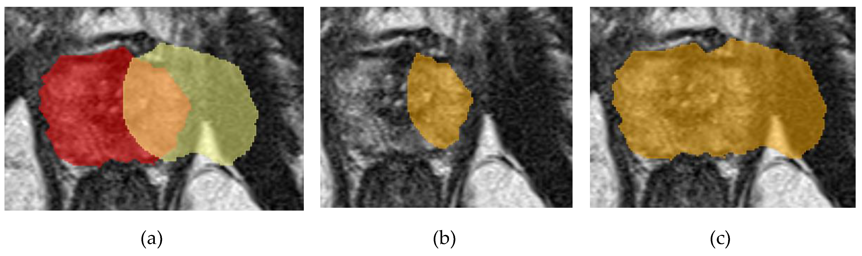
Figure 2.
Example of detection using YOLO.
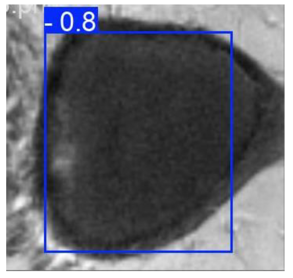
Figure 3.
Schematic of the preliminary-stage algorithm using one series as an example.
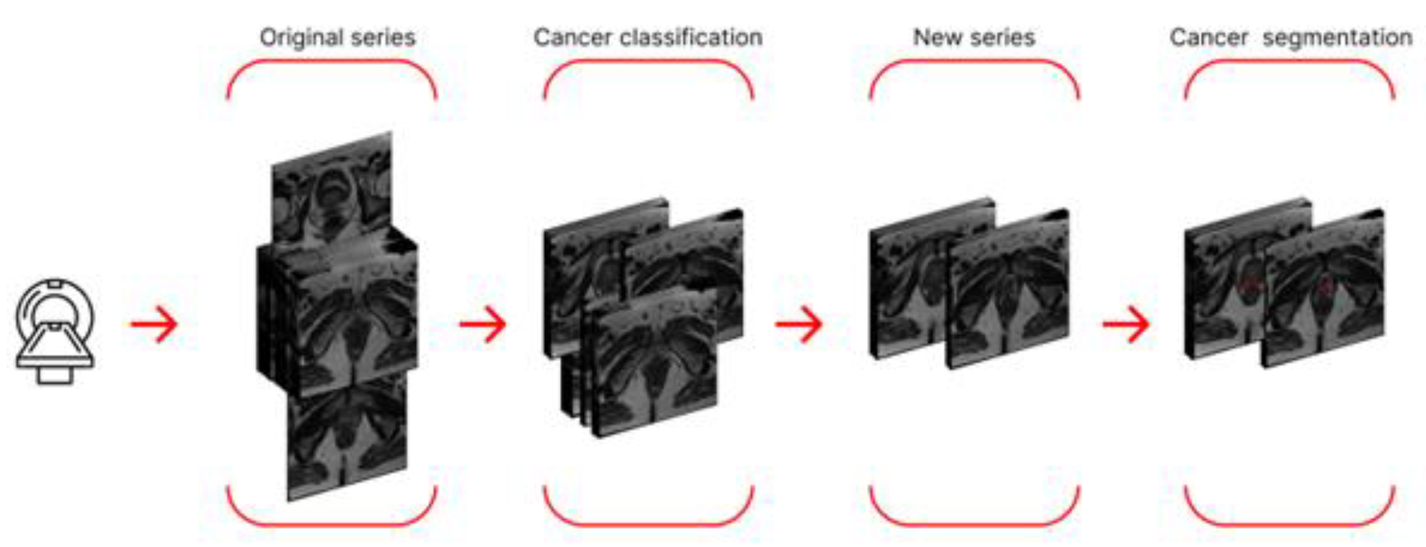
Figure 4.
Schematic representation of the algorithm using the prostate classification network in the main stage using a single series as an example.
Figure 4.
Schematic representation of the algorithm using the prostate classification network in the main stage using a single series as an example.
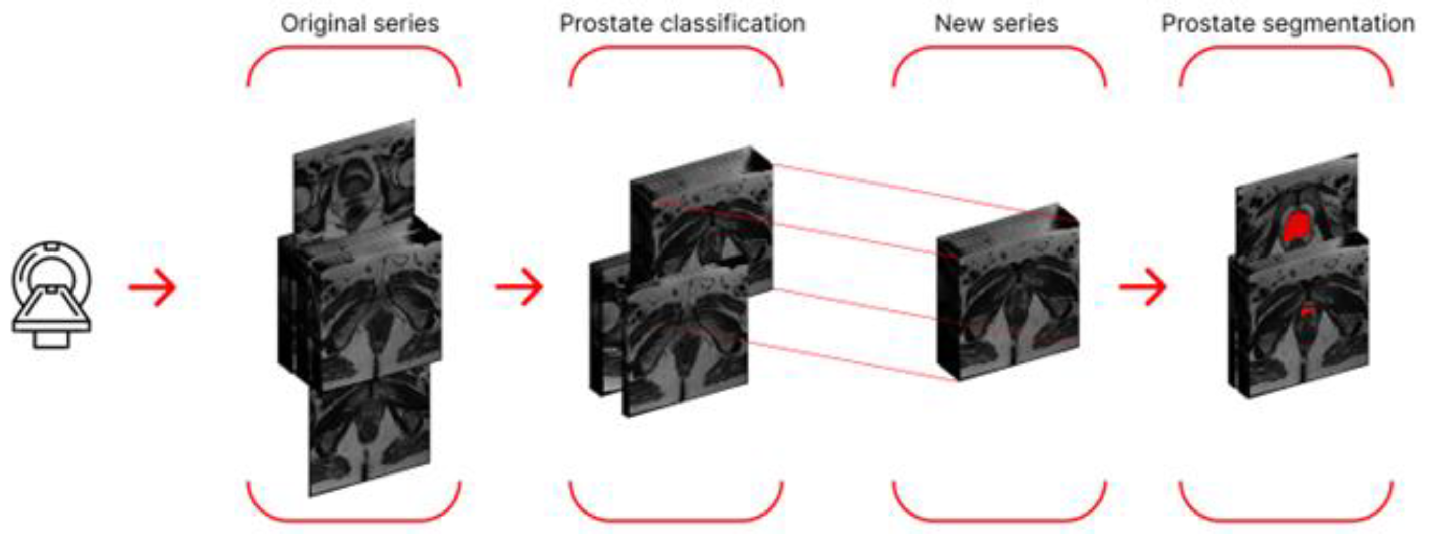
Figure 5.
Schematic representation of the algorithm using the prostate detection network in the main stage.
Figure 5.
Schematic representation of the algorithm using the prostate detection network in the main stage.
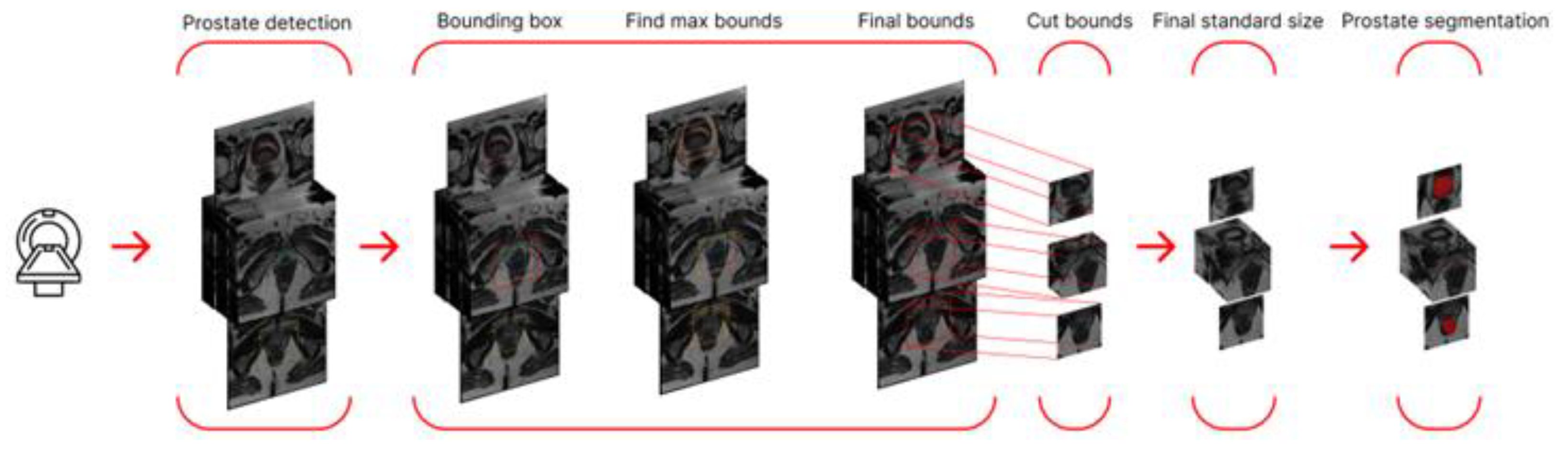
Figure 6.
Schematic representation of the final algorithm for the final stage.
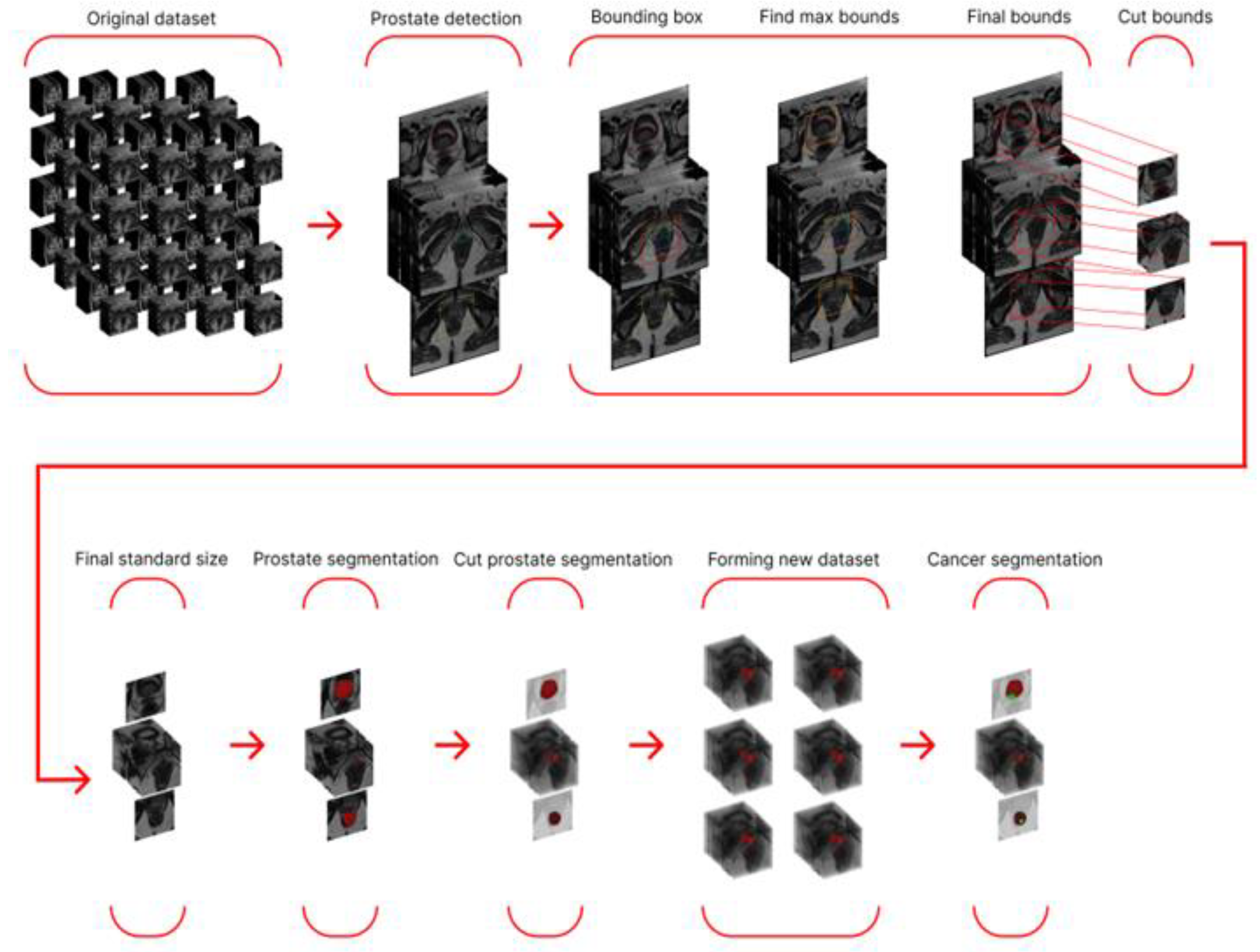
Figure 7.
Training graphs of the DenseNet-201 neural network: (a) dependence of the error on the training epoch; (b) dependence of the AUC on the training epoch.
Figure 7.
Training graphs of the DenseNet-201 neural network: (a) dependence of the error on the training epoch; (b) dependence of the AUC on the training epoch.
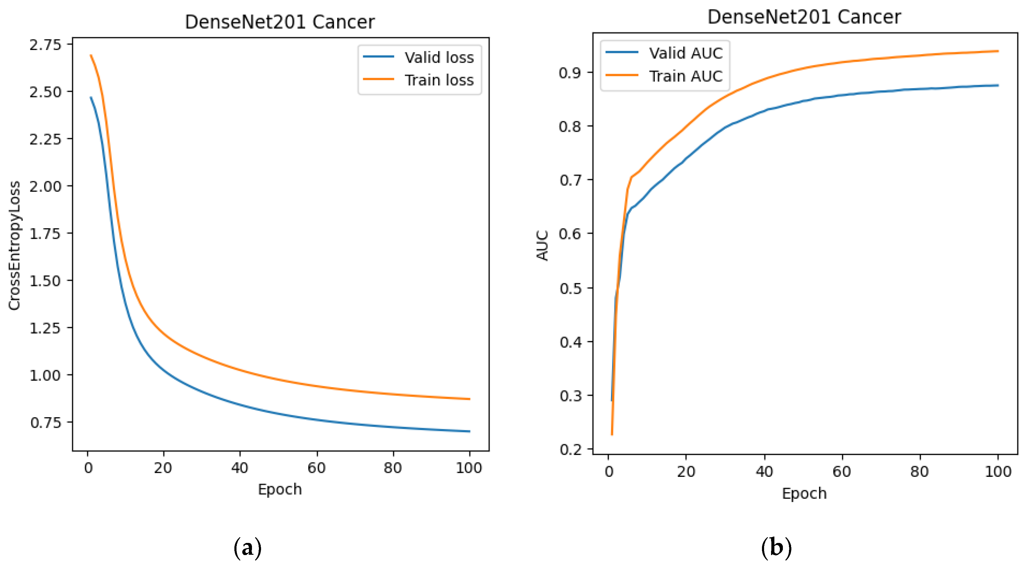
Figure 8.
Training graphs of the DenseNet-201 neural network: (a) dependence of the error on the training epoch; (b) dependence of the AUC on the training epoch.
Figure 8.
Training graphs of the DenseNet-201 neural network: (a) dependence of the error on the training epoch; (b) dependence of the AUC on the training epoch.
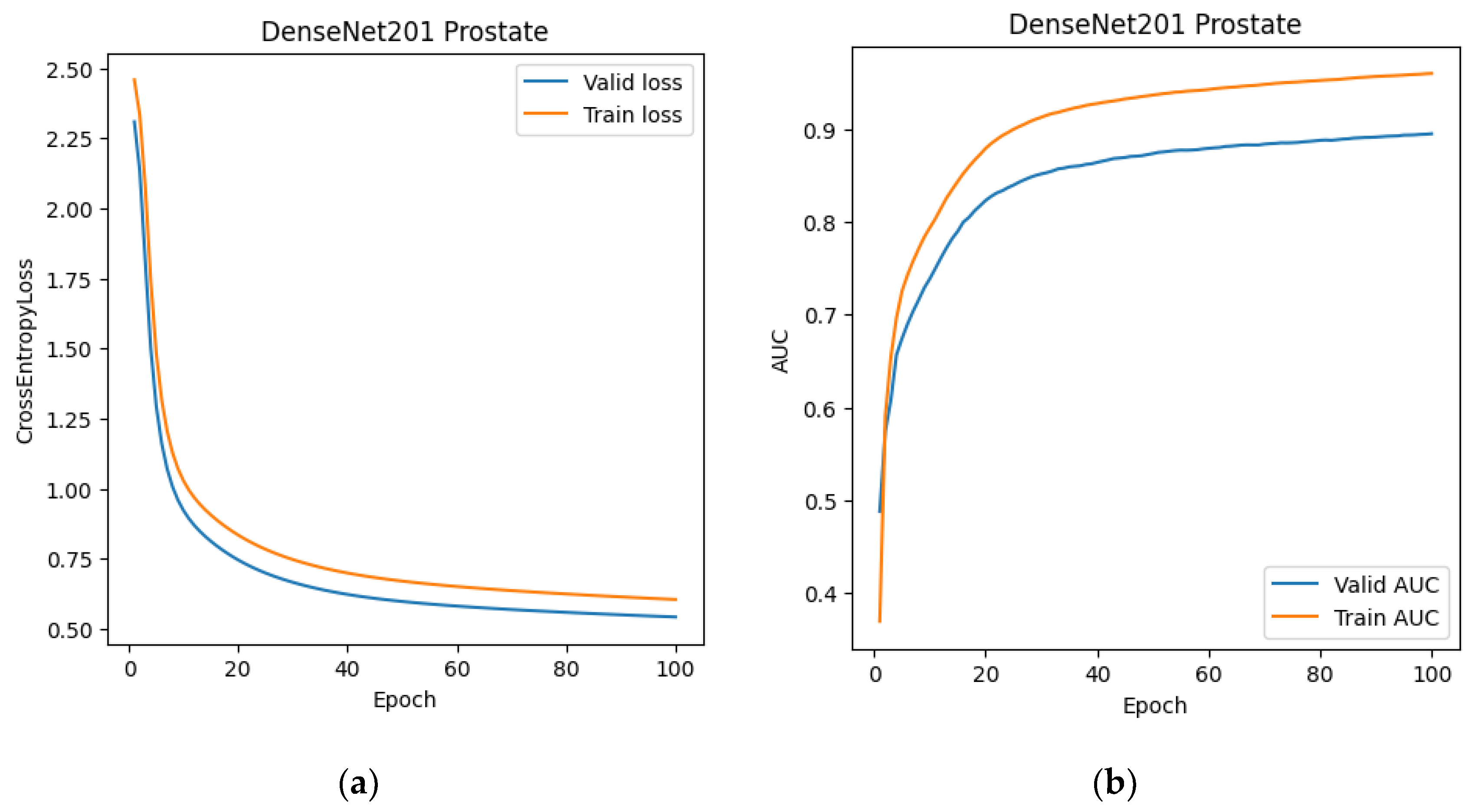
Figure 9.
Standard set of YOLO metrics after training.
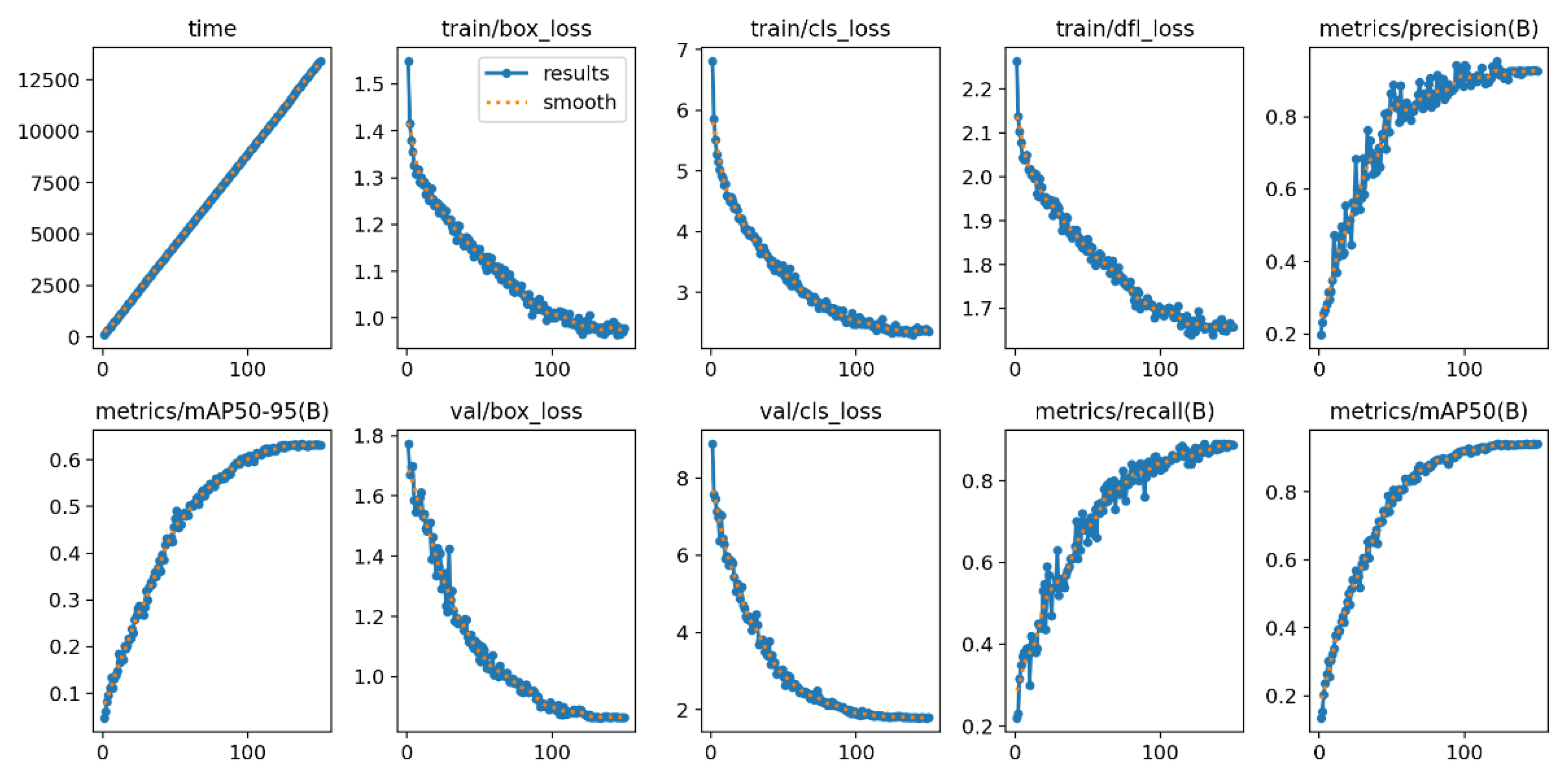
Figure 10.
Graphs of Dice change during training of the 2D Swin-UNETR network at the preliminary and main stages: (a) Dice change from epoch to epoch on the training set; (b) Dice change from epoch to epoch on the validation set.
Figure 10.
Graphs of Dice change during training of the 2D Swin-UNETR network at the preliminary and main stages: (a) Dice change from epoch to epoch on the training set; (b) Dice change from epoch to epoch on the validation set.
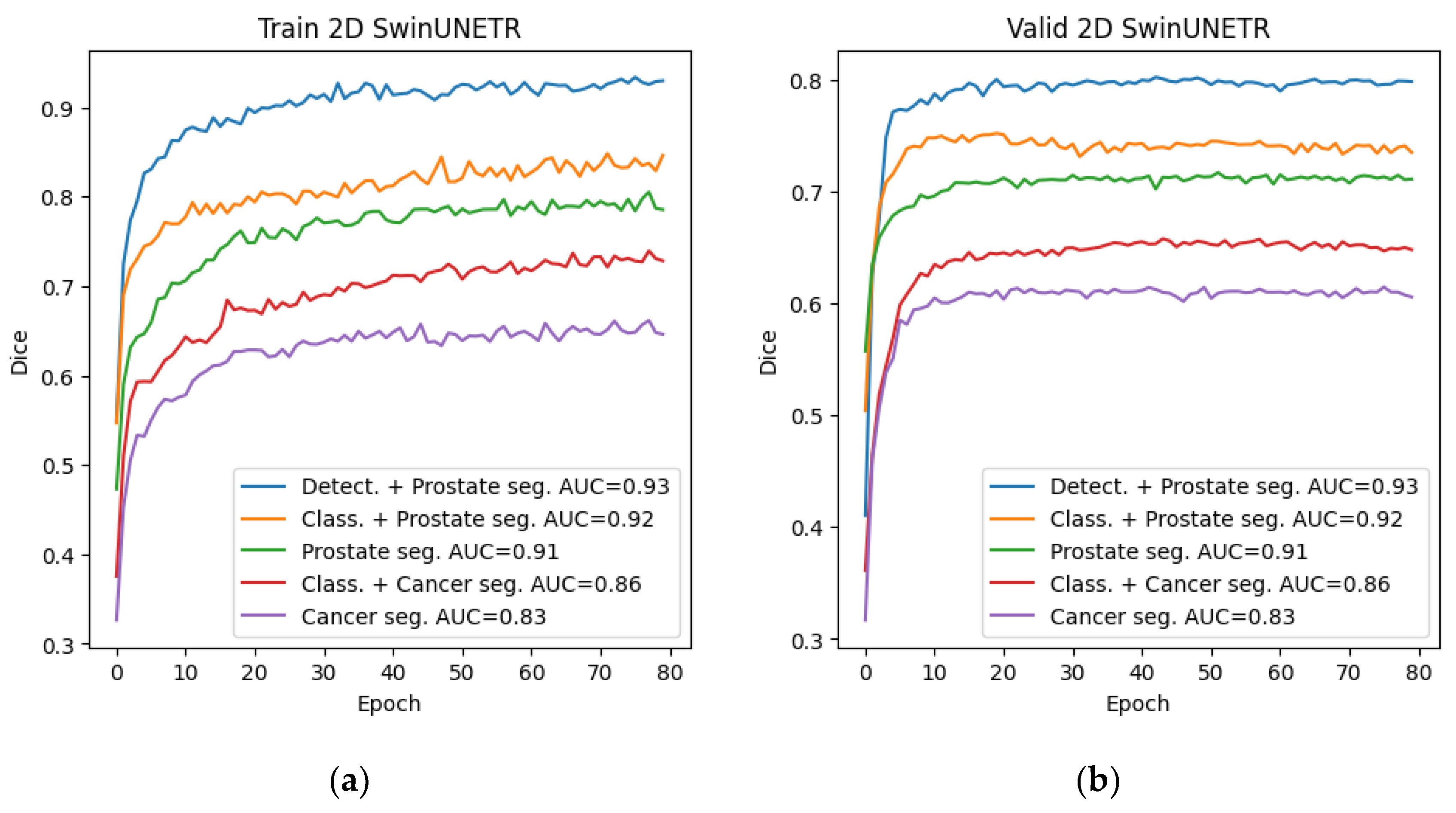
Figure 11.
Graphs of Dice change during training of the 2D Swin-UNETR network at the preliminary and main stages: (a) Dice change from epoch on the training set; (b) Dice change from epoch on the validation set.
Figure 11.
Graphs of Dice change during training of the 2D Swin-UNETR network at the preliminary and main stages: (a) Dice change from epoch on the training set; (b) Dice change from epoch on the validation set.
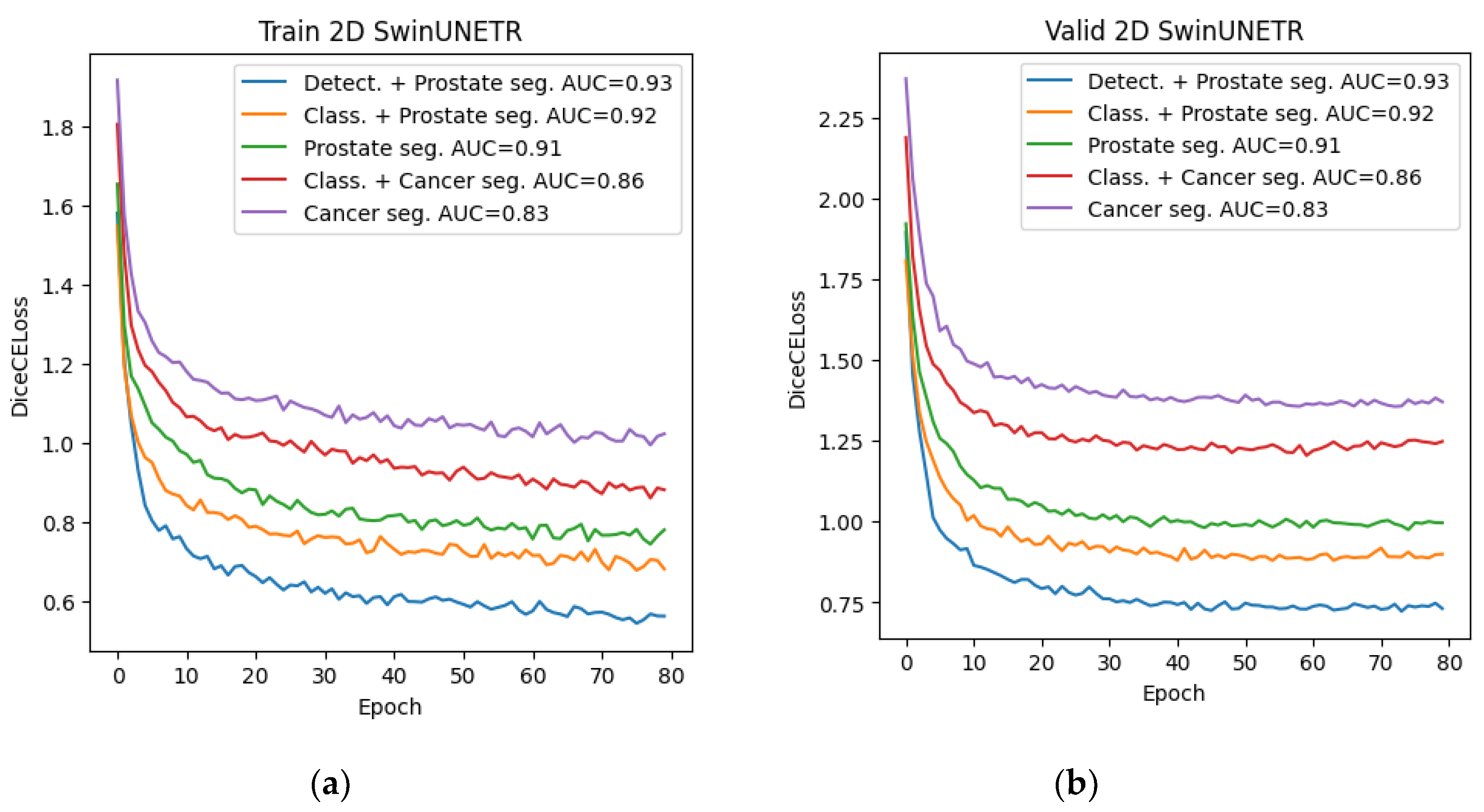
Figure 12.
Graphs of Dice changes during training of the 3D Swin-UNETR network at the preliminary and main stages: (a) Dice change from epoch to epoch on the training set; (b) Dice change from epoch to epoch on the validation set.
Figure 12.
Graphs of Dice changes during training of the 3D Swin-UNETR network at the preliminary and main stages: (a) Dice change from epoch to epoch on the training set; (b) Dice change from epoch to epoch on the validation set.
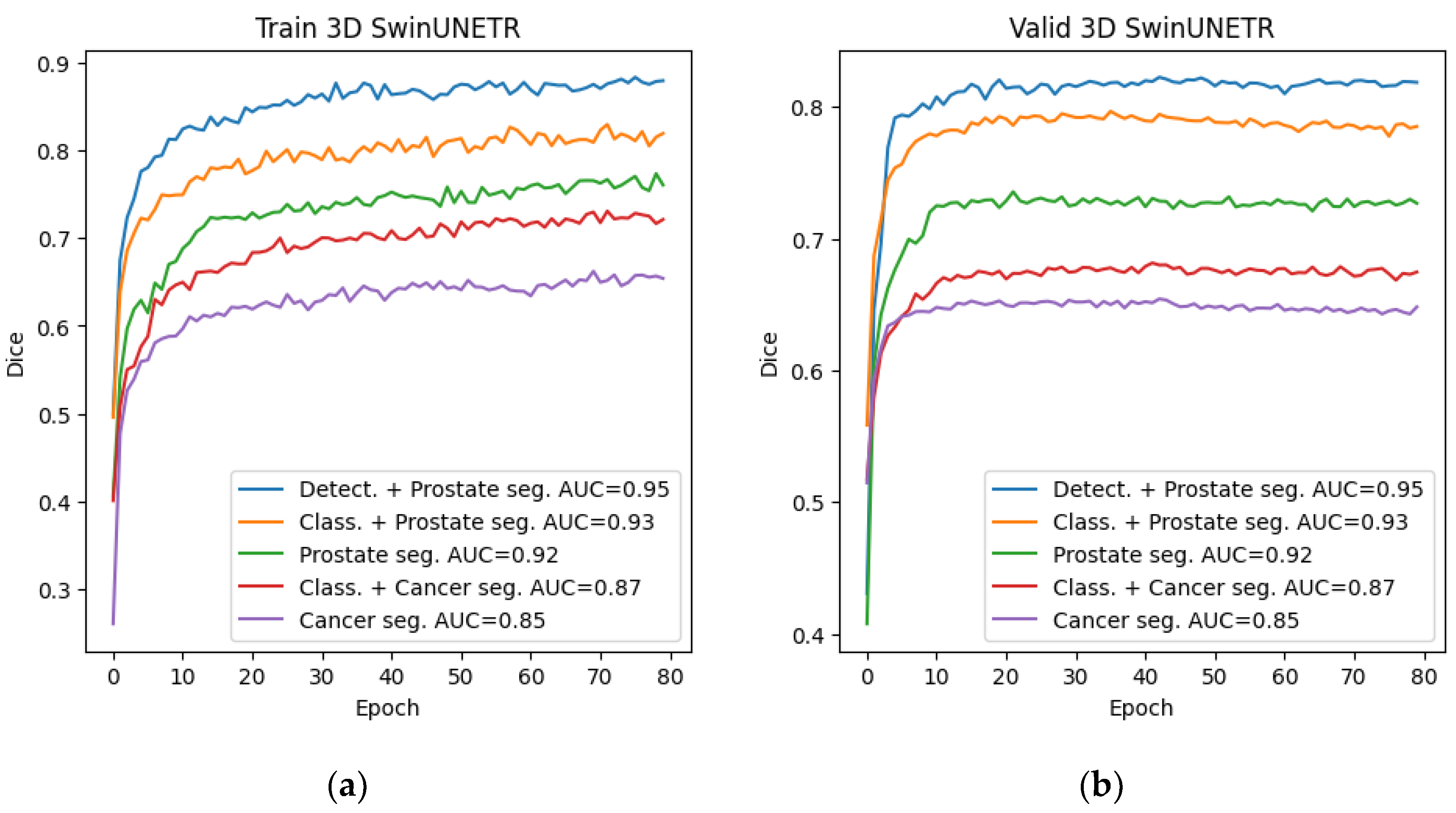
Figure 13.
Graphs of Dice changes during training of the 3D Swin-UNETR network at the preliminary and main stages: (a) Dice change from epoch on the training set; (b) Dice change from epoch on the validation set.
Figure 13.
Graphs of Dice changes during training of the 3D Swin-UNETR network at the preliminary and main stages: (a) Dice change from epoch on the training set; (b) Dice change from epoch on the validation set.
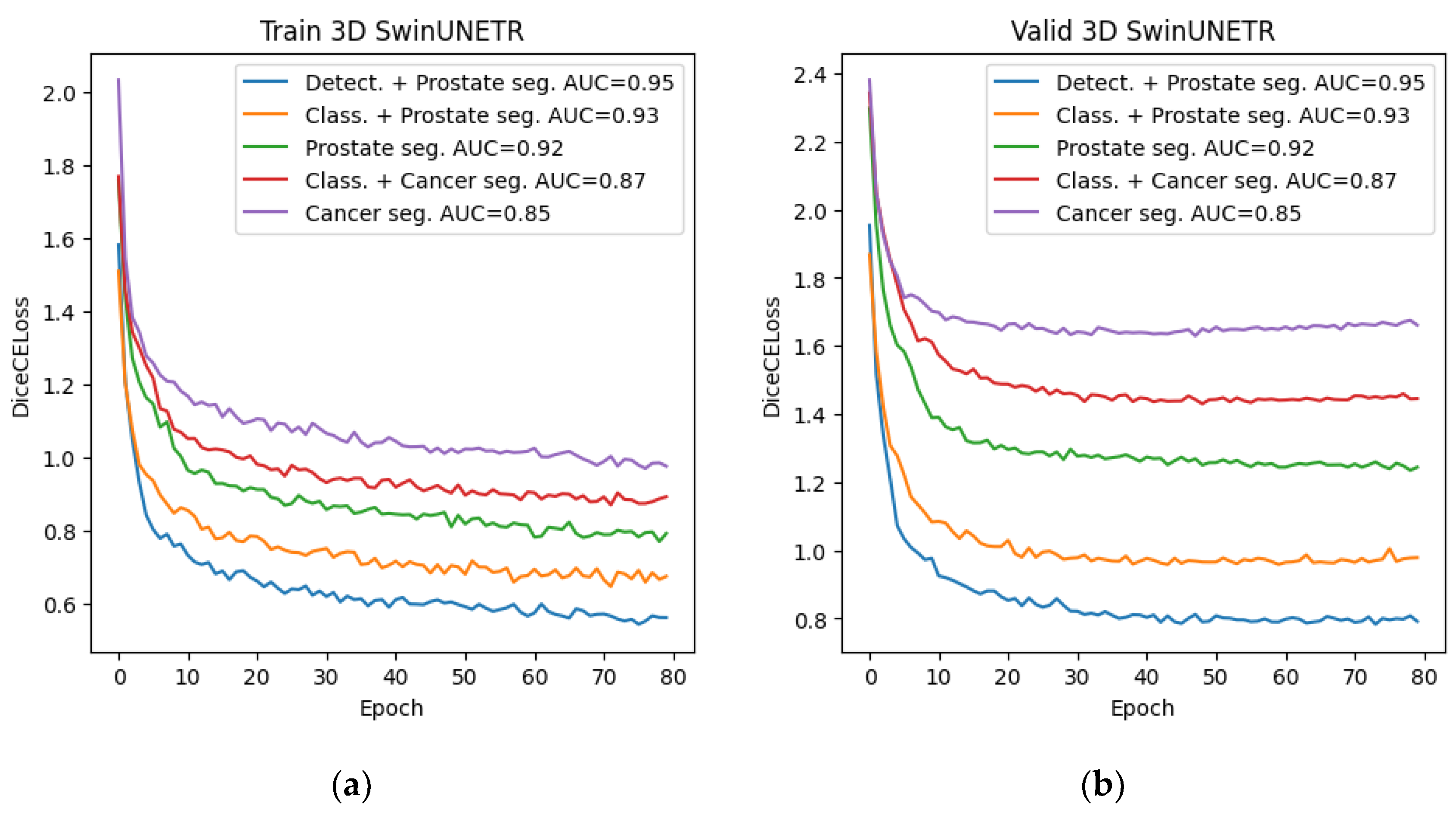
Figure 16.
AUC metric for Swin-UNETR networks trained at the final stage.
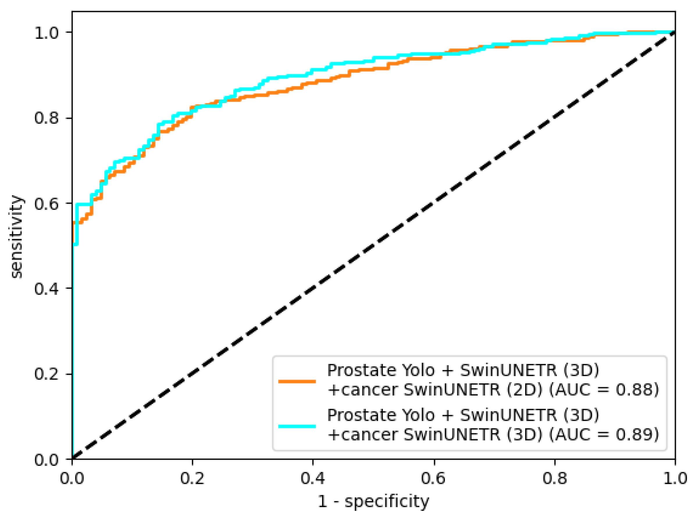
Figure 17.
Segmentation of cancer by the final 2D segmentation model.
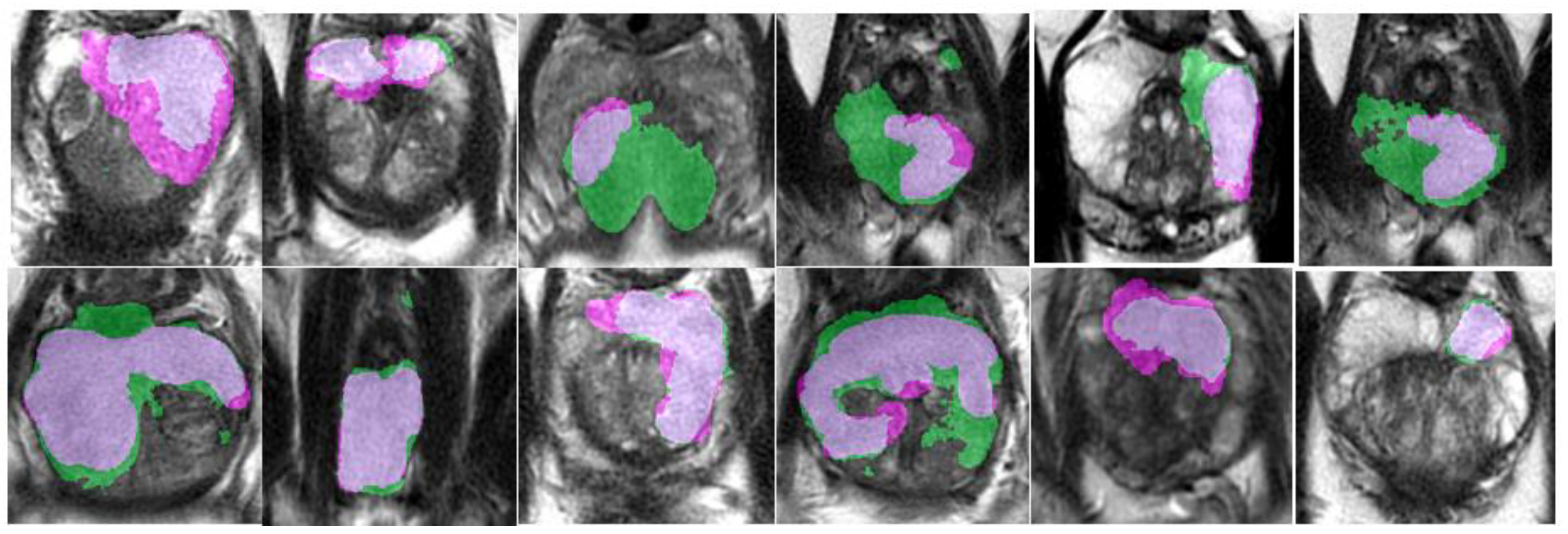
Figure 18.
Segmentation of cancer by the final 3D segmentation model.
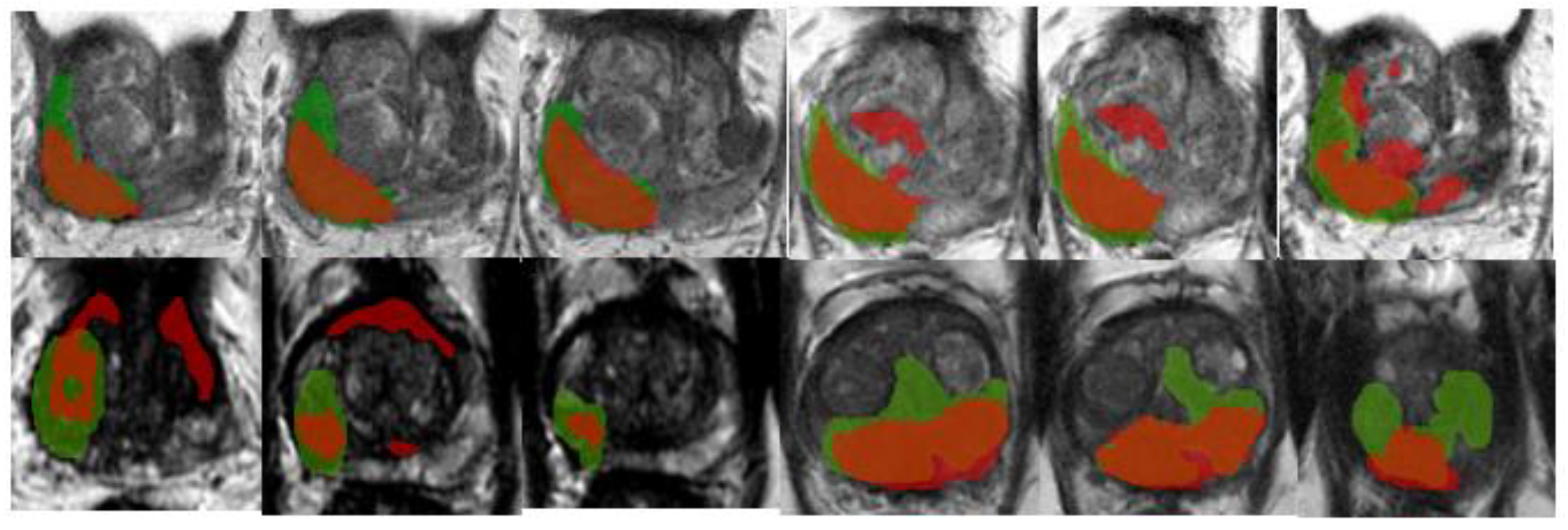
Table 2.
Server configuration for training.
| Hardware | Description |
| CPU | Intel(R) Xeon(R) Silver 4214R |
| GPU | NVIDIA RTX A6000 |
| RAM | 320 GB DDR4 |
Table 3.
YOLO configuration.
| Net configuration | Value |
| img_size | 312 x 312 |
| in_channels | 1 |
| output_channels | 1 |
| feature_size | 48 |
Table 4.
Final metrics of the models.
| Stage | Method | Architecture | metric | ||||||
| Dice, % | ROC AUC | Accuracy | Precision | Recall | Specificity | F1 | |||
| Stage 1 | 2D seg. | UNETR | 53.11 | 0.8 | 65.5 | 0.68 | 0.6476 | 0.6632 | 0.6634 |
| UNET++ | 54.16 | 0.81 | 67.25 | 0.7 | 0.6635 | 0.6825 | 0.6813 | ||
| Swin-UNETR | 54.89 | 0.83 | 68.25 | 0.705 | 0.6746 | 0.6911 | 0.6895 | ||
| 3D seg. | UNETR | 53.46 | 0.82 | 65.75 | 0.61 | 0.674 | 0.6438 | 0.6404 | |
| Swin-UNETR | 55.03 | 0.85 | 73.25 | 0.65 | 0.7784 | 0.6996 | 0.7084 | ||
| SegResNetDS | 53.18 | 0.83 | 69.25 | 0.625 | 0.7225 | 0.6696 | 0.6702 | ||
| SegResNetVAE | 53.26 | 0.83 | 70.5 | 0.615 | 0.75 | 0.6737 | 0.6758 | ||
| class. + 2D seg. | UNETR | 55.84 | 0.85 | 68 | 0.71 | 0.6698 | 0.6915 | 0.6893 | |
| UNET++ | 56.69 | 0.86 | 69.25 | 0.725 | 0.6808 | 0.7059 | 0.7022 | ||
| Swin-UNETR | 57.13 | 0.86 | 70.25 | 0.735 | 0.6901 | 0.7166 | 0.7119 | ||
| class. + 3D seg. | Swin-UNETR | 58.28 | 0.87 | 75.75 | 0.675 | 0.8084 | 0.721 | 0.7357 | |
| SegResNetDS | 56.93 | 0.86 | 73.25 | 0.665 | 0.7688 | 0.7048 | 0.7131 | ||
| Stage 2 | 2D seg. | UNETR | 65.85 | 0.88 | 75 | 0.785 | 0.7336 | 0.7688 | 0.7585 |
| UNET++ | 67.37 | 0.9 | 76 | 0.795 | 0.743 | 0.7796 | 0.7681 | ||
| Swin-UNETR | 68.22 | 0.91 | 77.5 | 0.82 | 0.7523 | 0.8022 | 0.7847 | ||
| 3D seg. | UNETR | 69.15 | 0.9 | 77.5 | 0.79 | 0.767 | 0.7835 | 0.7783 | |
| Swin-UNETR | 71.37 | 0.92 | 79.25 | 0.805 | 0.7854 | 0.8 | 0.7951 | ||
| SegResNetDS | 70.54 | 0.91 | 78 | 0.795 | 0.7718 | 0.7887 | 0.7833 | ||
| SegResNetVAE | 67.93 | 0.89 | 76.75 | 0.78 | 0.761 | 0.7744 | 0.7704 | ||
| class. + 2D seg. | UNETR | 67.32 | 0.9 | 80 | 0.83 | 0.783 | 0.8191 | 0.8058 | |
| UNET++ | 68.02 | 0.91 | 80.5 | 0.825 | 0.7933 | 0.8177 | 0.8088 | ||
| Swin-UNETR | 69 | 0.92 | 81.75 | 0.83 | 0.8098 | 0.8256 | 0.8198 | ||
| class. + 3D seg. | Swin-UNETR | 73.41 | 0.93 | 85.25 | 0.865 | 0.8439 | 0.8615 | 0.8543 | |
| SegResNetDS | 72.9 | 0.91 | 85.25 | 0.855 | 0.8507 | 0.8543 | 0.8529 | ||
| detect. + 2D seg. | UNET++ | 68.45 | 0.92 | 82.5 | 0.835 | 0.8186 | 0.8316 | 0.8267 | |
| Swin-UNETR | 69.94 | 0.93 | 83.75 | 0.845 | 0.8325 | 0.8426 | 0.8387 | ||
| detect. + 3D seg. | Swin-UNETR | 76.09 | 0.95 | 86 | 0.865 | 0.8564 | 0.8636 | 0.8607 | |
| SegResNetDS | 74.43 | 0.94 | 84.75 | 0.855 | 0.8424 | 0.8528 | 0.8486 | ||
| Stage 3 | detect. + 3D seg. + 2D seg. | Swin-UNETR | 66.23 | 0.88 | 75.25 | 0.76 | 0.7488 | 0.7563 | 0.7543 |
| detect. + 3D seg. + 3D seg. | Swin-UNETR | 67.11 | 0.89 | 76.75 | 0.765 | 0.7688 | 0.7662 | 0.7669 | |
Disclaimer/Publisher’s Note: The statements, opinions and data contained in all publications are solely those of the individual author(s) and contributor(s) and not of MDPI and/or the editor(s). MDPI and/or the editor(s) disclaim responsibility for any injury to people or property resulting from any ideas, methods, instructions or products referred to in the content. |
© 2025 by the authors. Licensee MDPI, Basel, Switzerland. This article is an open access article distributed under the terms and conditions of the Creative Commons Attribution (CC BY) license (http://creativecommons.org/licenses/by/4.0/).
Copyright: This open access article is published under a Creative Commons CC BY 4.0 license, which permit the free download, distribution, and reuse, provided that the author and preprint are cited in any reuse.


