
Submitted:
19 December 2025
Posted:
22 December 2025
You are already at the latest version
Abstract
This study investigates the application of the Mumford-Shah functional, a foundational variational model in image segmentation, to the challenge of Land Use/Land Cover (LuLc) mapping within an Object-Based Image Analysis (OBIA) framework. Recognizing that no single segmentation algorithm is universally optimal, the research focuses on comparing two distinct numerical approximations to assess their suitability for processing satellite imagery. The methodological approach involved the systematic evaluation of two algo-rithms: the Ambrosio-Tortorelli method and the Active Contour Snake model. To ensure controlled conditions, a series of synthetic test images were created, featuring basic geo-metric shapes representing common landscape features. These images were designed across multiple scenarios, ranging from those with clean, high-contrast edges to more challenging cases with low contrast and introduced intra-class noise, simulating re-al-world complexities. The performance of each algorithm was rigorously measured using established statistical metrics, namely Cohen's Kappa and the Jaccard Index, to quantify segmentation accuracy against a known ground truth. The findings reveal a clear distinc-tion in algorithmic behavior. While both methods achieved high accuracy in ideal, high-contrast conditions, their performance diverged significantly under stress. The Am-brosio-Tortorelli algorithm proved notably more robust, effectively maintaining closed and coherent object boundaries even in the presence of noise and low spectral contrast. Conversely, the Snake model was highly sensitive to these conditions, often resulting in fragmented contours or complete failure to delineate objects. In conclusion, this compara-tive analysis demonstrates that the choice between these two approaches is not arbitrary but critically dependent on the nature of the input data. The study provides practical guidance, suggesting that the global, variational approach of Ambrosio-Tortorelli is better suited for the noisy and spectrally complex scenes often encountered in territorial analy-sis. Meanwhile, the Snake model may be reserved for more controlled scenarios with sharp, well-defined edges. This work thus contributes a reasoned framework for algorithm selection, aiming to enhance the precision and reliability of segmentation in sustainable landscape monitoring workflows.
Keywords:
mumford-shah functional
; image segmentation
; object-based image analysis (OBIA)
; land use / land cover (LULC) mapping
; variational methods
; ambrosio-tortorelli approximation
; active contour models (snakes)
; algorithm comparison / performance benchmarking
1. Introduction
Accurate and detailed knowledge of Land Use and Land Cover (LULC) is one of the most significant areas of interest in spatial planning and landscape science. It inherently involves diverse research fields, from the strictly ecological to the technological [1,2], and holds central importance in a wide range of studies and applications. These include urban planning, natural and environmental resource monitoring, land-use policy development, and even in understanding global climate evolution [3].
LULC classifiers can be distinguished as either supervised or unsupervised [4] and as parametric or non-parametric [5,6].
The first distinction is based on whether a dataset is required to train the classification algorithm. In practice, supervised algorithms are provided with input data alongside the correct corresponding outputs—for instance, ‘this pixel with these characteristics is grassland.’ The algorithm thus learns the relationship between input and output and replicates this procedure across the entire dataset to be analysed. In contrast, unsupervised algorithms do not require a preliminary dataset for training; instead, they autonomously identify patterns, similarities, and clusters within the dataset under analysis [7] (Lu & Weng, 2007).
Algorithms can further be distinguished as parametric or non-parametric. The key discriminator here is the requirement for a strong preliminary assumption about the statistical distribution of the data [5], typically assumed to be Gaussian for parametric methods. For non-parametric algorithms, these initial assumptions are unnecessary, making them considerably more adaptable in situations where in-depth prior knowledge of the analysis area is lacking [8].
These two broad categories are not mutually exclusive but rather intersect, providing a deeper interpretative framework for the tools. In this sense, we can identify algorithms that are: Supervised Parametric, Supervised Non-Parametric, Unsupervised Parametric, and Unsupervised Non-Parametric (see Table 1).
As can be observed from Table 1, there is currently access to a significant and heterogeneous range of algorithms. However, there is still no single ideal or universally superior algorithm in terms of robustness and result accuracy [9]. In other words, there is no perfect algorithm, only the one most suited to a specific problem, dataset, user skill level, and final objective, in line with the “No Free Lunch Theorem” formulated by Wolpert in 1995 [10,11].
This principle implies that an algorithm’s superiority only emerges in specific contexts, as its performance results from a trade-off between bias, variance, and computational complexity [12]. Consequently, the relative performance of algorithms is strictly dependent on the nature of the dataset, the size of the training set, and the specific characteristics of the thematic classes to be distinguished [13].
Furthermore, LULC recognition algorithms can be used individually, following the well-established pixel-based technological approach, or they can be associated with, and applied consecutively to, more specific image segmentation methods (Figure 1) within the more recent theoretical and technological paradigm of Object-Based Image Analysis (OBIA) [14].
More specifically, the former classifies each pixel based on its spectral signature, which in many cases generates classifications affected by noise, producing a ‘salt-and-pepper’ effect [15]. Conversely, in the second possibility—the OBIA approach—the image is first segmented into homogeneous regions (objects) that correspond to real-world entities, distinguishing them from what could be termed the “background.” Subsequently, a semantic classification is performed based not only on the spectral characteristics of these objects, but also on their shape, texture, and context [16].
Although algorithms can be effectively employed in both approaches, comparative studies have shown that OBIA surpasses pixel-based methods in accuracy, particularly when using high-resolution imagery and classifying complex categories, such as those in urban environments [17]. However, in this case as well, the choice between the two approaches is not a matter of “right or wrong,” or “better or worse,” but of fitness for purpose. The pixel-based approach is simpler, more direct, and often sufficient for medium-to-low-resolution data where the goal is a general estimate of land cover; whereas an OBIA approach is preferable when working with very high-resolution imagery, such as that acquired by drones [18], and/or in situations where the classes to be distinguished have similar spectral signatures but different shapes or textures. Examples include distinguishing a roof from a road [19] or differentiating between tree species, where, in some cases, texture features are more important than purely spectral ones [20].
Following the OBIA procedure flow (Figure 1), it becomes clear that the choice of segmentation algorithm is crucial for the final quality of the objects. It is upon these objects that, in the subsequent phase, semantic classification will be applied using the algorithms previously described.
A detailed examination of various segmentation algorithms and their applications is provided in the edited volume by Blaschke et al. (2008) [16], which compiles several pioneering works in the field. It delves into the theoretical foundations of segmentation and the concept of scale within the principal and most widely used algorithms. A thorough exploration and classification of these would warrant a dedicated discussion. However, a sufficiently general synthesis can be attempted, starting from the seminal and foundational research by Haralick & Shapiro (1985) [21], which categorises these algorithms into logical families based on their operating principles (Figure 2).
The first family comprises algorithms that operate on the direct detection of edges (Edge Detection), identifying them where a significant gradient in brightness/colour is measured. For instance, Jin & Davis (2005) [22] utilised techniques from this family to identify building outlines using high-resolution imagery, demonstrating the utility of these algorithms within an OBIA workflow for land analysis.
The second family (Region Growing) includes algorithms that function in a diametrically opposite manner to the former. Instead of seeking edges, they directly seek homogeneous areas. More specifically, they start from a ‘seed pixel’ and iteratively aggregate adjacent pixels that meet a similarity criterion, for example, a spectral difference below a certain threshold. A valid and widespread example of this family is the Multiresolution Segmentation developed by Baatz & Schäpe (2000) [23], which simultaneously considers spectral and shape similarity.
A third family incorporates clustering techniques that group pixels based on statistical parameters. For example, the K-Means algorithm [24,25], despite its simplicity, remains a benchmark for this technique, although it requires the a priori definition of the number of clusters (K). A more robust and non-parametric evolution is represented by the Mean-Shift algorithm [26], which automatically determines the number of clusters by seeking the modes in the dataset’s density distribution.
The last category encompasses more modern and specialised algorithms. These develop techniques to model the physical properties of the scene, such as illumination or reflectance, to separate objects. Others are based on Graph-Based approaches, which represent the image as a graph where nodes are pixels and edges connect neighbours; similarity between pixels is assigned to the edge as a weight attribute, and segmentation occurs by removing edges with minimal weight, thereby partitioning the graph [27,28].
Also, within this last family, one finds techniques based on Mixture Models, which assume the data is generated from a mixture of statistical distributions, where each mixture component represents an image region with distinct statistical properties [29].
Of course, from 1985 to the present day, theoretical and technological progression has made significant advances, and the kaleidoscope of algorithms has grown considerably. For example, Pal & Ghosh (1992) [30] explicitly acknowledge the role of fuzzy set theory in segmentation; subsequently, Cheng et al. (2001) [31] focus on colour image segmentation, incorporating specific methods, such as those based on colour physics, separating reflectance components from illumination to achieve segmentation more robust to changes in light, shadows, and reflections.
Furthermore, the advent of Deep Learning has revolutionised the playing field, developing methods capable of learning hierarchical features according to neural network architectures (e.g., FCN, U-Net), marking a significant leap forward in performance (Garcia et al., 2017) [32]. For conceptual accuracy, Deep Learning technology, like Fuzzy logic or Graph Theory itself, could be considered as transversal tools, potentially applicable to all classical segmentation families, rather than as criteria for generating new families. For instance, one could operate with a Region-Based approach, automated via a convolutional neural network that incorporates Fuzzy logic.
An additional class of tools can be identified in variational methods or energy-based models. This class distinguishes itself from the previous ones through its more strictly mathematical and geometric approach to the segmentation problem. Its seminal representative can be found in the Mumford-Shah functional [33]. Through energy optimisation, it allows the image to be segmented into homogeneous regions by differentiating its pixels into those belonging to a “smooth” zone, such as the interior of a sought-after object or the image background, and those identifying the separation, or more precisely, the boundary between objects and background.
The technique of image segmentation via this procedure occurs by minimising the energy value produced by the pixels of an image. However, minimising the Mumford-Shah functional directly is highly complex because the set of object boundaries can have wide variability. Minimising the functional means finding the best segmentation of an image that balances three objectives [34]:
a) having smooth regions, inside of which there are no large variations in the image; thus, low variance between pixel values.
b) having boundaries that are as short and regular as possible.
c) the processed image, where pixels are classified as boundary or background, must resemble the original image as closely as possible.
In more formal terms, for an original two-dimensional image , one seeks an image that simplifies and a set of boundaries , which minimise the overall energy as in the following (equation 1):
The first part of the equation, known as the regularity term, “penalises” variation within the smooth regions. In other words, the simplified image should be as uniform as possible inside each region, such as the interior of an object or the background itself.
The second term controls the fidelity, or more precisely, the similarity between the original image and its simplified copy , through the tuning parameter . Assuming a high value for this parameter forces the objects in the copy to be characterised by a high level of detail. However, this inevitably leads to an increase in the length of the segmentation boundary and, consequently, in the overall energy value .
Finally, the last part of the functional penalises overly long and complex boundaries through the parameter . Increasing this parameter produces solutions with shorter and simpler contours [35], but conversely, there is a risk of losing useful details that are not merely “noise.”
The original formulation of the problem by Mumford and Shah stipulates that must be a finite union of closed, regular (more precisely, analytic) curves. However, as is customary in modern Mathematical Analysis, it is preferable to work with a version where such regularity is not directly required. One can then attempt to prove that the minimising sets are, in fact, more regular, using their minimality to demonstrate this. For generic sets , the concept of length can be generalised using one-dimensional Hausdorff measure. With this nuance, for each fixed , the functional can be minimised with respect to the variable in a classical manner, using appropriate Sobolev spaces, to obtain minimisers . The subsequent minimisation—that is, minimising with respect to —is more complex and requires considering the Hausdorff convergence of sets and the minimality properties of the solution [36]. Solving minimisation problems involving the Mumford-Shah functional in the presented form is therefore extremely complex, as it involves two variables, the function and the set , of very different natures.
A completely different viewpoint is due to De Giorgi, who interprets the variable as the sole variable of the problem, with the set replaced by the set of essential discontinuity points of . To implement this approach, appropriate spaces of Special functions of Bounded Variation (from which the acronym SBV is derived) were introduced and studied. Using these, the functional can be defined as follows (equation 2):
This represents the weak form of the Mumford-Shah functional, where is replaced by and a suitable meaning is given to the “approximate gradient,” allowing for the resolution of the related minimisation problems. Furthermore, regularity theorems then ensure that can be considered as a union of curves [37,38,39]. Despite this conceptual effort, the implementation of a direct numerical minimisation of the Mumford-Shah functional—even via the De Giorgi method—still presents significant difficulties. These stem from its dependence on the unknown one-dimensional set , whether considered as an arbitrary closed set or as a finite union of closed curves.
However, the formulation in terms of SBV functions allows the functional to be framed within a variational setting. In this setting, one can construct approximations capable of guaranteeing the convergence of the minimisation problems, understood as the convergence of both the minimal values and the minimising functions. A sequence of functionals possessing this property is said to Gamma-converge to [40]. This approach offers greater flexibility, which translates into the possibility of developing approximations in spaces different from that of the Gamma-limit—in our case, the Mumford-Shah functional in its weak form [41].
In this research, an approximation technique for the Mumford-Shah functional and a dynamic approach directly aimed at the recognizing contours will be implemented to test their potential and limitations in recognising objects within raster images. These two solutions, which can be succinctly referred to as Ambrosio-Tortorelli and Snakes, will be explained in detail in the following section.
2. Methods
2.1. Formatting of Mathematical Components
Among the various solutions for numerically approximating the Mumford-Shah functional, the one proposed and studied by Ambrosio and Tortorelli has been particularly widely used, especially in computational contexts [37]. The core idea behind this approximation is the use of an additional variable or parameter: a function , such that is a “regularised” version of the characteristic function of the discontinuity set . In essence, the function takes the value 1 “far” from the discontinuity set of , and 0 “close” to it. The “regularized” term (equation 3) is:
is thus well-defined even if the function u is discontinuous on S(u), meaning that over this set the product with v2 is null. The term involving the length of S(u) is replaced with a continuous approximation dependent on the parameter n, with n tending to infinity (equation 4):
For large n, the finiteness of the first term in this integral implies that v is close to the constant 1 except on a set of small measures. Recalling that the value of v is 0 on S(u), this means the function v must undergo a transition from 0 to 1 in a neighbourhood of S(u). This transition, however, is penalised by the second integral. As n tends to infinity, these two terms balance each other, and their combined value tends to a multiple of the length of S(u), due to a Gamma-convergence result related to phase transitions [42].
The Ambrosio-Tortorelli functional, dependent on the parameter n, thus takes the overall form (equation 5):
The characteristic of the Ambrosio-Tortorelli functional that makes it particularly suitable for numerical approximation is that, while not being a convex functional of the pair, it is a separately elliptic functional in both variables and . This property allows the easy application of discretisation methods. It should be noted that the functional is defined on pairs (u,v); therefore, one must formally consider pairs of convergent functions (un,vn). However, the limit is meaningful only if is an almost everywhere approximation of equation 1, meaning the limit is defined only on pairs (u,1). On such pairs, it takes the value of the Mumford-Shah functional . In this sense, we have the Gamma-convergence of the Ambrosio-Tortorelli functionals to the Mumford-Shah functional. Therefore, for a good approximation of the solutions to the Mumford-Shah functional, it will be sufficient to compute numerically approximate solutions for the Ambrosio-Tortorelli functional with a sufficiently high control parameter , which is linked to the mesh step size. The results obtained through the Ambrosio-Tortorelli procedure can be compared with those from other mathematical models developed for segmentation problems. Specifically, we will use the Active Contour Snake procedure, or more simply Snakes, as a comparative solution. The broader objective is to identify which types of shapes are energetically favoured by the mathematical structure of the involved minimisation problems, in order to develop an optimal selection criterion.
In formal terms, a Snake is a closed, regular parametric curve that minimises an energy composed of:
- Internal energy, which maintains the curve’s regularity.
- External energy, which attracts the curve towards the edges in the image.
The internal energy consists of a length term and a curvature term (representing tension and flexibility, respectively). Minimising the internal energy alone, with constant coefficients, produces regular curves known as elastica. The external energy depends on the image via its gradient and is minimised where the gradient is greatest—that is, on the contours of objects within the image. Thus, the external energy alone is minimised by curves that position themselves as much as possible along the image edges. Therefore, the result is determined by a competition between ’s attraction to the contour and the minimisation of the boundary’s length and curvature.
The minimisation of a Snake’s energy is achieved through an evolutionary approach by introducing a time variable and a Snake that evolves according to the gradient flow of the energy, i.e., a parabolic equation (in the case of constant and ) of the type (equation 6):
with an initial “guess” condition , where is a “regularised” version of the image from the Mumford-Shah problem formulation. This scheme produces a limiting snake as tends to infinity, which corresponds to a stationary point of the energy, and thus potentially a (local) minimum. Clearly, the solution depends essentially on the choice of , which must “surround” the sought-after contour. Therefore, the gradient flow scheme must be repeated several times, with different initial guesses, to obtain a minimal (and not resulting from other stationary points) and complete description. Unlike the previous solution, the Snake yields a result solely in terms of the object contours within the image and does not employ an image fidelity term. Consequently, it does not provide an output image outside the set of contours . Furthermore, the parameterisation of the Snake as a closed curve makes this method more effective for the contours of convex objects.
2.2. Algorithmic Implementation
Following the solution proposed by Ambrosio and Tortorelli, we must find the function (the approximated image) and the function (the edge map) that minimise the value of . The numerical implementation follows these logical steps:
- a)
- Initialisation:
- A matrix u(x,y) is created to approximate the original image g(x,y) as closely as possible. The ideal initial solution is therefore to initialise u(x,y) with the exact numerical values of g(x,y).
- For the function v, which will contain the edge map, a matrix of the same dimensions as u(x,y) is initialised, with all its elements assigned the value v=1. Starting with the value 1 everywhere means assuming, in the initial phase, that there are no edges in the image—a neutral starting hypothesis. In subsequent iterations, the algorithm will update this matrix, pushing values towards the threshold 0 to identify discontinuities (i.e., the edges of the sought objects).
- b)
- Iterative Minimisation; once the matrix is initialised, the functional is minimised through an iterative process:
- Minimise with respect to u: The values in the matrix u(x,y) are updated, using the current v matrix (initially all 1s).
- Minimise with respect to v: Using the newly computed u(x,y) matrix from the previous step, the functional is minimised again, this time with respect to v. This yields an updated edge map matrix v.
- c)
- Convergence: these alternating minimisations between the and matrices are repeated until the changes in the respective updated matrices are deemed negligible.
A simple flowchart, as shown in Figure 3, can aid in understanding this procedure.
Specifically, the minimisation of u(x,y) with respect to v is implemented via the Euler–Lagrange equation for u (in discrete form), which yields a linear system whereby each element of the matrix u(x,y) is updated as a function of its neighbours. For each pixel, a new value is then computed, balancing the original datum and the regularisation term (equation 7)
where *h* is the spatial step (h=1) and, in the case of the first iteration where v=1 everywhere, the expression simplifies to an average between the datum and the mean of its neighbours. Conversely, for the minimisation of v with respect to the updated u(x,y), the formula derived from the per-pixel minimisation of the matrix (equation 8) is used:
where the squared magnitude ∣∇u∣² is obtained using the centered finite-difference scheme to compute the partial derivatives (equation 9):
It should be recalled that in regions where the gradient is high, v becomes small (<<1), allowing u(x,y) to approach the original data more closely in subsequent iterations.
At the start of the algorithm, i.e., just prior to initialising the first matrices, it is necessary to assign values to the control parameters mentioned previously: µ, ν, K. There is no predetermined rule or single criterion for their setting; their initialisation is often based on experience and on values found in the literature, or on a preliminary visual analysis of the image. Table 2 below provides some general guidelines for their configuration. The choice of control parameters is frequently also the result of an iterative “trial and error” adjustment or an automated search – for example, using a test image with a known “ground truth” segmentation to find the parameters that maximise accuracy. As stated, different parameters will yield slightly different results (e.g., sensitive edges, sharper or smoother transitions). However, although the parameters are chosen arbitrarily in the initial stage, the logic of the algorithm is to automatically balance the terms of the functional due to the form of the minimisation equations.
Regardless of the procedure leading to the initial setting of these parameters, the logic guiding the choice remains the same.
Regarding parameter , it should be remembered that for low values of the algorithm will be more sensitive and precise in following jagged edges and complex details; conversely, a high value makes the algorithm less sensitive, producing smoother and more regular edges, but at the risk of cutting out fine details. This occurs because, recalling the structure of the functional in equation 1, parameter directly multiplies the contour length . This term represents the “cost” of having a contour:
- If is LOW (e.g., ): The “cost” of a long contour is low. The algorithm is not heavily penalised for creating jagged and complex contours to follow every small detail or variation in the data.
- If is HIGH (e.g., ): The “cost” of a long contour is high. The algorithm will be strongly penalised if it creates a complex contour. It will therefore seek the solution with the shortest and simplest possible contour, even if this means approximating the data slightly less accurately. The result will be smoother, more regular, and “minimal” edges. In other words, the algorithm will suppress small details and noise but may also cut out genuine corners or fine details.
In addition to these parameters, we must also consider K, which is a composite parameter that encapsulates the combined influence of µ, ϵ, and ν, as established in the earlier Formula 8. A value for K can be considered “good” if it generates a useful transition for the variable v. To illustrate, if the gradients ∣∇u∣² are on the order of 10⁶, then a value like K=0.02 would be far too small. In this scenario, the product K⋅∣∇u∣² would be enormous everywhere, forcing v to be approximately zero across the entire field and thus rendering its variation largely meaningless. Conversely, if the gradients ∣∇u∣² are on the order of 10³, that same K=0.02 would be excessively large. The product K⋅∣∇u∣² would then be close to zero everywhere, constraining v to be approximately one throughout, which again yields a non-informative result. In summary, the initial parameter selection should aim to scale K such that the product K⋅∣∇u∣² is very large for strong gradients (indicating true edges) and very small for weak gradients (such as those associated with a high level of noise).
For the algorithmic implementation of the Snake, it must first be recalled that it is a parametric curve which minimizes a total energy computed as (equation 10):
where v(s) = (x(s), y(s)) represents the parametric curve of the contour. The internal energy governs the geometric properties of the Snake according to (equation 11):
Considering a set of N points vₖ = (xₖ, yₖ), the derivatives can be approximated using finite differences as (equation 12):
From these, the form of Discrete Internal Energy can be derived as (equation 15):
The parameters α and β represent, respectively, the tension and the flexibility of the curve. One can conceptualise α as a kind of spring connecting consecutive points along the Snake, whose function is to keep them evenly spaced. The parameter β, on the other hand, governs flexibility. It can be explained by imagining a kind of rigid bar that resists bending; its role is to strive to make the Snake as smooth and regular as possible.
Here too, the initial setting of these parameters depends on a series of subjective considerations by the operator. The key aspects of these considerations are summarised in the following two tables (Table 3 and Table 4).
External energy is formally defined as (equation 14):
whose partial derivative discretization, with respect to x and y respectively, are given by (equation 15 and 16) where H and W denote the height and width, respectively, of the image matrix:
3. Material, Experiment and Results
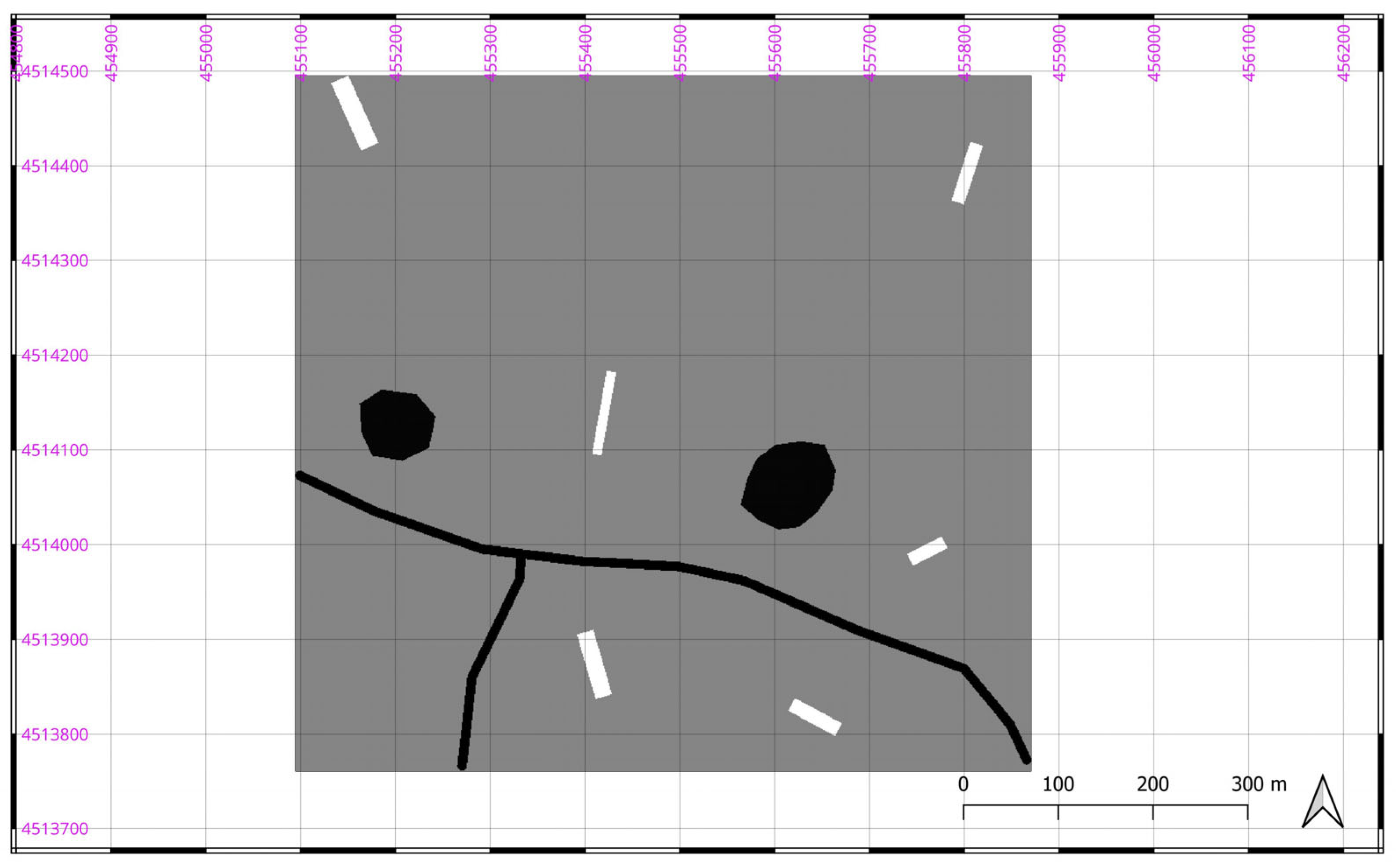
To evaluate the performance of the two procedures and the algorithmic efficiency achieved through their implementation in the Python™ programming language, it was decided to test the Ambrosio–Tortorelli model and the Snake on a library of images specifically generated for this purpose. These images were created within the QGIS environment (https://qgis.org/) starting from vectorised elementary shapes, typically representative of common geographic features such as roads, buildings, trees, or small bodies of water (Figure 4). Using this type of imagery, albeit very simple, offers the advantage of having full control over the results obtained from the Ambrosio–Tortorelli model and the Snake. Indeed, by assuming these base images to be the “ground truth,” the precise location and semantic classification of each pixel are known with absolute certainty, as they were generated according to predetermined specifications.
These original images can therefore be reliably used as reference bases against which to assess the algorithms’ ability to determine the shape, size, and position of the objects contained within the images.
Subsequently, the original image was converted into a raster-type matrix, with a pixel resolution of 1m × 1m, resulting in a total of 760 × 760 pixels. Thus, the image matrix comprises 577,600 elements in total. Each pixel was then assigned an energy value through a greyscale (0–255), determined by its spatial position—specifically, whether the pixel was located inside one of the circulars, rectangular, or polygonal shapes, or outside of them. For this first experimental step, it was hypothesised that the circular shapes could represent trees, the rectangles buildings, the polygon a road, and all pixels not included within these geometries were classified as background. Ten test scenarios were then generated by assigning a specific greyscale energy value to each object class. This value differed between pixels belonging to different object classes but was uniform for pixels within the same class. Furthermore, the energy value assigned to each class was scaled to achieve an overall variance of the entire image matrix that increased progressively from Scenario 1 to Scenario 10, as detailed in the subsequent Table 5. Having obtained the initial results, which will be examined and discussed in detail later, it was decided to increase the complexity within the original image to understand the current limitations of the algorithmic solutions. For this reason, a further 9 scenarios were generated. In these, variance in the energy value was also introduced within objects belonging to the same geometric class. This was achieved using a “random” function with predetermined bounds, as outlined in the subsequent Table 6.

Table 5.
The ten scenarios featuring constant energy within each class and differing energy between classes.
Table 5.
The ten scenarios featuring constant energy within each class and differing energy between classes.
| Scenario | Trees | Buildings | Roads | Background | Global Variance |
| S1 | 67 | 77 | 65 | 73 | 12 |
| S2 | 62 | 82 | 60 | 73 | 25 |
| S3 | 57 | 87 | 55 | 73 | 45 |
| S4 | 52 | 92 | 50 | 73 | 85 |
| S5 | 47 | 97 | 45 | 73 | 165 |
| S6 | 42 | 102 | 40 | 73 | 330 |
| S7 | 37 | 107 | 35 | 73 | 660 |
| S8 | 32 | 112 | 30 | 73 | 1230 |
| S9 | 27 | 117 | 25 | 73 | 2640 |
| S10 | 22 | 122 | 20 | 73 | 5280 |
Figure 5.
The overall raster image matrix (760px × 760px) with energy values assigned to the pixels according to scenario S10. Processed by the Authors.
Figure 5.
The overall raster image matrix (760px × 760px) with energy values assigned to the pixels according to scenario S10. Processed by the Authors.
Following the acquisition of results from both the Ambrosio-Tortorelli model and the Snake algorithm for these scenarios as well, the evaluation of object recognition and segmentation performance across the different described scenarios was undertaken. This assessment employed several statistical metrics, including Cohen’s Kappa [43] and the Jaccard Index [44].
Table 6.
The nine scenarios with noise were introduced both within and between classes.
| Scenario |
Trees (range) |
Buildings (range) |
Roads (range) |
Background (range) |
Global Variance |
| S1_R | 28-32 | 118-122 | 208-212 | 69-71 | 450-500 |
| S2_R | 25-35 | 115-125 | 205-215 | 68-72 | 550-650 |
| S3_R | 20-40 | 110-130 | 200-220 | 66-74 | 800-1000 |
| S4_R | 15-45 | 100-140 | 190-230 | 63-77 | 1500-2000 |
| S5_R | 8-50 | 90-150 | 180-240 | 60-80 | 2500-3500 |
| S6_R | 18-42 | 105-135 | 195-215 | 69-71 | 700-900 |
| S7_R | 22-38 | 112-128 | 205-215 | 68-72 | 600-750 |
| S8_R | 24-36 | 116-124 | 202-218 | 67-73 | 500-600 |
| S9_R | 26-34 | 116-124 | 206-214 | 68-72 | 480-520 |
Figure 6.
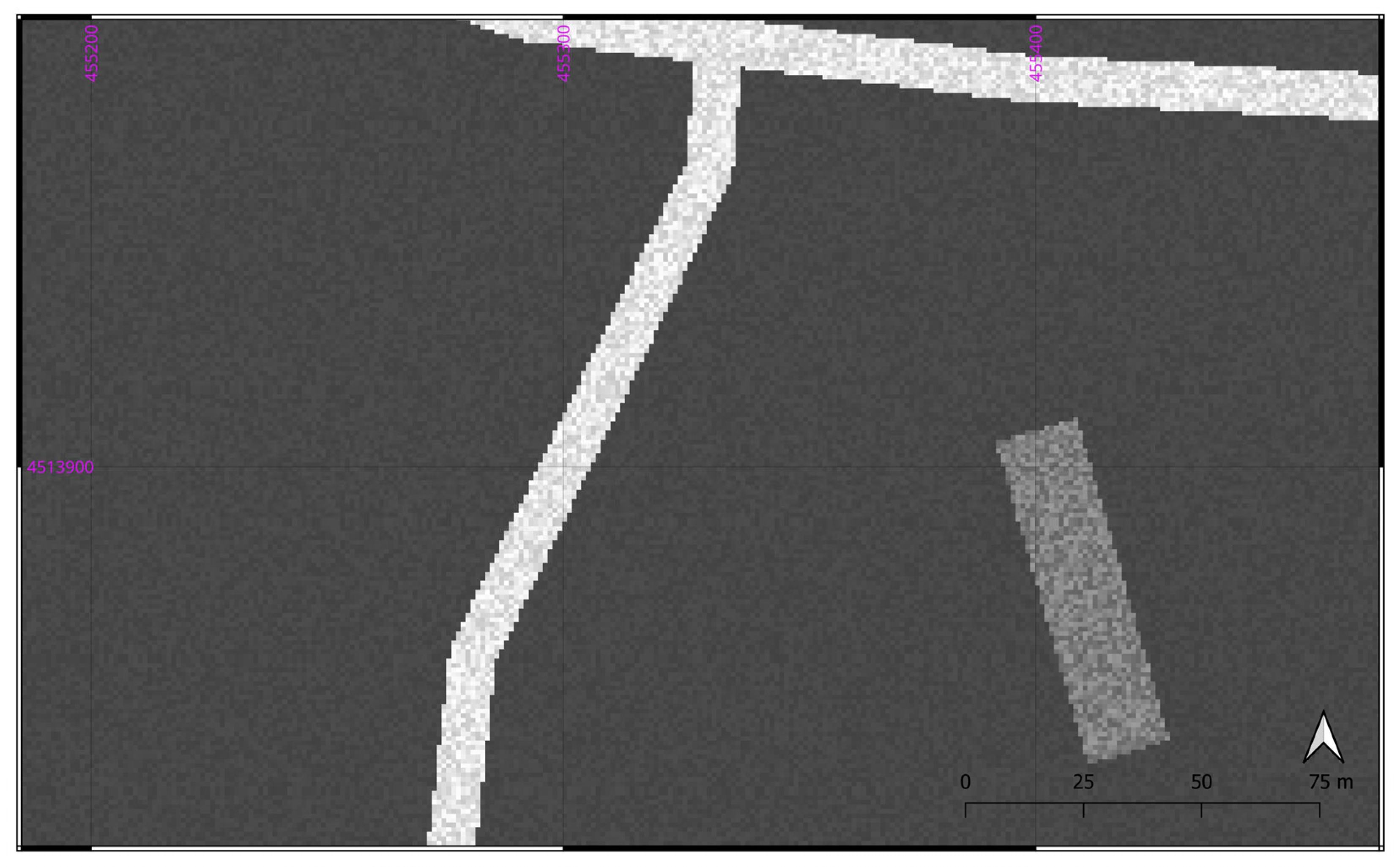
Detail of the raster image matrix developed according to the parameters of scenario S9_R. It can be observed how the value assigned to the pixels tends to vary within the geometric shapes. Processing by the Authors.
Figure 6.
Detail of the raster image matrix developed according to the parameters of scenario S9_R. It can be observed how the value assigned to the pixels tends to vary within the geometric shapes. Processing by the Authors.
The former estimates the measure of agreement between two raters and is formally expressed as (equation 17):
where ωₒ denotes the observed agreement—that is, the agreement observed between the two raters, calculated as the ratio of all concordant judgments to the total number of judgments. The term ωₑ expresses the value of the expected agreement, i.e., the agreement that would be expected if the two raters were statistically independent, maintained the same observed marginal distributions, and responded randomly. This approach is considered robust because it provides the percentage of agreement corrected for the component of chance agreement. In other words, it answers the question: “What percentage of the observed agreement is NOT explainable by mere chance?”
The second statistical metric, the Jaccard Index, measures the similarity between two sets based on the positions of the “1”s in the two matrices. This second evaluator is particularly useful when the “1” values are relatively rare, are considered more important for the analysis, and one wishes to estimate the overlap of the “1” areas. Formally, the Jaccard Index can be expressed as (equation 18):
In this context, A∩B corresponds to the number of positions where both matrices have the value “1”, while A∪B represents the number of positions where at least one of the two matrices records a “1”. Within the framework of this research, the role of the two “raters” is played, on one side, by the original image matrix and, on the other, by the matrices produced by the Ambrosio-Tortorelli and Snake algorithms. To conduct this final comparative analysis, it was necessary to convert all image matrices into binary matrices. In these, value 0 was assigned to background pixels and the value 1 to all pixels belonging to an object, regardless of their class. This transformation is an essential prerequisite for making the results comparable. While this conversion was straightforward for the original matrices, it presented greater complexity for the results obtained from the Ambrosio-Tortorelli model. This algorithm identifies pixels of strong discontinuity but does not directly provide a continuous, closed boundary delineating an object. Furthermore, an additional ambiguity arises it is necessary to specify to the system whether the object of interest is the area enclosed by the boundary pixels or the area outside them—to use a metaphor, whether one is seeking the doughnut or the doughnut hole. To overcome these two issues, two additional Python™ scripts were developed. The first task is to connect the boundary pixels into a continuous and closed path, even when discontinuities exist between them. In practice, when a pixel with a value of 1 is not adjacent to another, the script searches for the nearest subsequent pixel, allowing for a maximum tolerable discontinuity of 5 pixels. The second script, conversely, identifies and assigns value 1 to all pixels located inside these closed paths. To determine whether a pixel is inside a contour, a horizontal line is traced from that pixel in one direction (right or left, it does not matter). If this line intersects an odd number of boundaries before reaching the edge of the matrix, the pixel is classified as inside an object; if the number of intersections is even, the pixel is considered part of the background.
The tests conducted on the first image library—specifically, the scenarios without energy variance within objects—seem to indicate that both procedures deliver highly satisfactory results. The Snake algorithm performed well in 9 out of 10 cases, and the Ambrosio-Tortorelli model in 10 out of 10, albeit with some reservations regarding scenario S1 (Table 7 and Table 8). It appears that when the energy gradient between objects, and between objects and the background, falls below a certain threshold, the algorithms exhibit greater uncertainty in the object recognition process. The subsequent image shows the analytical graphical result of the Ambrosio-Tortorelli model applied to S1 (Figure 7). It can be observed that it fails to recognise the rectangular objects, yet it still yields a more effective outcome than the Snake algorithm, which in this case does not recognise a single object.
The situation changes dramatically when energy variance is introduced within objects, yet again with significant differences between the two algorithms. Except for scenario S5_R, where the intra-object variance reaches its maximum value, the Ambrosio-Tortorelli model demonstrates consistent performance across all scenarios. Naturally, the values for both Cohen’s Kappa and the Jaccard Index are significantly lower than in the previous, simpler scenarios. The Snake algorithm, however, appears to be more sensitive to the variance parameter (Table 9 and Table 10). It must also be noted that while the Ambrosio-Tortorelli model, despite evident difficulties, recognises and segments some objects largely in their original entirety, the Snake algorithm seems only to identify certain fragments. The subsequent analyses of the analytical graphical results illustrate these differences more effectively.
The subsequent Figure 8 shows the results of the Ambrosio-Tortorelli model for scenario S1_R: it recognizes the road but loses all other features. Nevertheless, by the end of the process, the road is successfully identified as a single, coherent object. Subsequently, Figure 9 shows the analytical graphical result of the Snake algorithm applied to the same scenario. As also indicated by the two statistical conformity estimators, there are no significant differences.
Effectiveness decreases significantly as variance increases. For example, consider scenario S4_R, which features high variance values—though not the maximum reached in this experiment. The Ambrosio-Tortorelli model works with consistent efficacy, as can be observed in the following images: it recognises the polygonal object as a single, unified entity. The Snake algorithm, on the other hand, also detects that there are other objects in the image, but it perceives them as fragmented—that is, it fails to establish continuity in their shape (Figure 10).
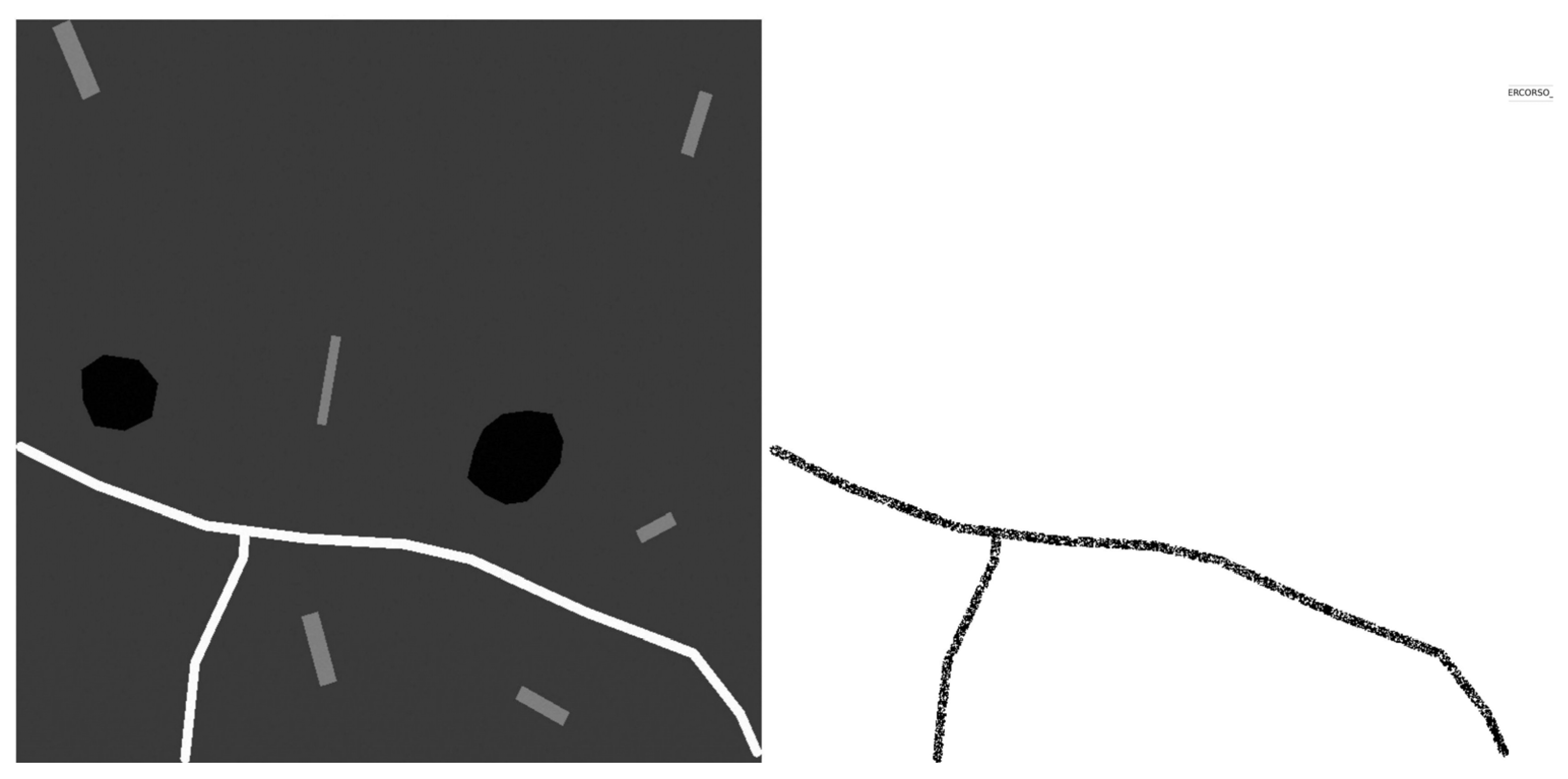
These differences between the two algorithms appear to diminish as the internal variance within objects decreases. Take scenario S3_R as an example: a certain degree of object fragmentation is still observed, although it is more contained; however, the perception that rectangular-shaped objects also exist is lost.
Figure 11.
Left: the original raster image for scenario S3_R. Right: the image reconstructed using the Snake model, showing the determination of edges and the pixels internal to the objects. Processing by the Authors.
Figure 11.
Left: the original raster image for scenario S3_R. Right: the image reconstructed using the Snake model, showing the determination of edges and the pixels internal to the objects. Processing by the Authors.
4. Discussion
This study has explored the application of the Mumford-Shah functional through two different numerical approximation techniques—the Ambrosio-Tortorelli (AT) method and the Active Contour Snake model—as potential tools to support satellite image segmentation for Land Use/Land Cover (LuLc) analysis within the Object-Based Image Analysis (OBIA) paradigm. From experimental results conducted on synthetic images with controlled complexity, significant differences emerge between the two methods, both in terms of numerical performance and algorithmic behavior.
It is essential to recall that these are still preliminary tests carried out on relatively simple and ad hoc objects; therefore, future work will involve analyses of real-world cases. The most notable strength of the AT method lies in its ability to identify an object’s boundary as a single, continuous entity, even when some pixels are missing. This stems from its mathematical formulation, which inherently identifies contrast in the presence of an object. In contrast, the Snake model, due to its evolutionary mathematical structure, tends to “skip over” potential boundaries when uncertain—for instance, in cases of low energy variance—and thus fails to recognize them. This phenomenon becomes more pronounced in noisy conditions, where AT still attempts to provide a global, albeit less detailed, response, while the Snake struggles significantly.
From a mathematical standpoint, both methods naturally face challenges in recognizing objects with low energetic variance, as they are built upon competing parameter families. It would likely be beneficial to adapt parameter settings regionally, differentiating them after an initial reconstruction—for example, by recalibrating parameters zone by zone following the initial identification of high-contrast areas.
In summary, in scenarios without internal noise, both methods achieve high accuracy levels when the energy differences between objects and background are sufficiently marked (scenarios S2–S10). However, in scenario S1, characterized by low energetic contrast, AT maintains an acceptable recognition capability, while the Snake fails completely, demonstrating greater sensitivity to weak gradients. When intra-class variance is introduced as noise, AT shows superior robustness, maintaining consistent performance across various noise levels (except in the extreme case S5_R). Conversely, the Snake exhibits a progressive decline in segmentation ability as noise increases, tending to fragment objects rather than delineate continuous contours.
Regarding output shape, AT tends to produce closed and continuous boundaries, identifying objects as unified entities even under noisy conditions. The Snake, on the other hand, may yield discontinuous or fragmented contours, especially where gradients are non-uniform or interrupted. The explanation for these behaviors lies in the fundamental nature of the two approaches: Ambrosio-Tortorelli is a static and global method, working simultaneously across the entire image by minimizing an energy functional that balances internal regularization, data fidelity, and contour length. Its variational nature makes it particularly suitable for identifying structures even in the presence of partial discontinuities. In contrast, the Snake is an evolutionary and local method, based on the dynamic evolution of an initial curve attracted by local gradients. This makes it more agile for well-defined, convex contours but also more vulnerable to noise, weak gradients, and the need for accurate initialization.
The results suggest that Ambrosio-Tortorelli may be preferable in contexts where the objects to be segmented exhibit low spectral contrast against the background, the presence of noise or variable internal texture, and the need for closed and topologically coherent contours. Conversely, Snakes can be effective in high-contrast scenarios with regular, convex-shaped objects, especially when supported by good initialization and well-calibrated parameters.
This research represents a preliminary investigation conducted on synthetic data. Future steps will require testing on real high-resolution satellite imagery, extending the analysis to more complex and irregular shapes typical of real landscapes, developing dynamic parameter adaptation based on local image characteristics—such as zone-by-zone calibration after initial region detection—and integrating post-processing techniques to regroup discontinuous boundaries (in the case of Snakes) and to enable semantic classification after segmentation.
In conclusion, the Mumford-Shah functional, in the two approximations tested here, confirms its potential as a powerful mathematical tool for segmentation within OBIA. The choice between AT and Snake is not absolute but depends on the application context, data quality, and required level of detail. Specifically, AT demonstrates greater reliability under noisy and low-contrast conditions, while Snakes can offer precision in more controlled and high-contrast scenarios. This work thus provides a solid comparative framework to guide the selection of segmentation algorithms based on the characteristics of the analyzed landscape, contributing to the optimization of workflows for sustainable landscape monitoring through remote sensing.
5. Patents
This section is not mandatory but may be added if there are patents resulting from the work reported in this manuscript.
Conflicts of Interest
“The authors declare no conflicts of interest.”.
References
- Abdi, A. M. Land cover and land use classification performance of machine learning algorithms in a boreal landscape using Sentinel-2 data. GIScience & Remote Sensing 2020, 57(1), 1–20. [Google Scholar]
- Yimer, S. M.; Bouanani, A.; Kumar, N.; Tischbein, B.; Borgemeister, C. Comparison of different machine-learning algorithms for land use land cover mapping in a heterogenous landscape over the Eastern Nile River basin, Ethiopia. Advances in Space Research 2024, 74(5), 2180–2199. [Google Scholar] [CrossRef]
- Schulz, D.; Yin, H.; Tischbein, B.; Verleysdonk, S.; Adamou, R.; Kumar, N. Land use mapping using Sentinel-1 and Sentinel-2 time series in a heterogeneous landscape in Niger, Sahel. ISPRS Journal of Photogrammetry and Remote Sensing 2021, 178, 97–111. [Google Scholar] [CrossRef]
- Saponaro, M.; Tarantino, E. LULC Classification Performance of Supervised and Unsupervised Algorithms on UAV-Orthomosaics. In International Conference on Computational Science and Its Applications; Springer International Publishing: Cham, July 2022; pp. 311–326. [Google Scholar]
- Qian, Y.; Zhou, W.; Yan, J.; Li, W.; Han, L. Comparing machine learning classifiers for object-based land cover classification using very high-resolution imagery. Remote sensing 2014, 7(1), 153–168. [Google Scholar] [CrossRef]
- Phiri, D.; Morgenroth, J. Developments in Landsat land cover classification methods: A review. Remote sensing 2017, 9(9), 967. [Google Scholar] [CrossRef]
- Lu, D.; Weng, Q. A survey of image classification methods and techniques for improving classification performance. International journal of Remote sensing 2007, 28(5), 823–870. [Google Scholar] [CrossRef]
- Shao, Y.; Lunetta, R. S. Comparison of support vector machine, neural network, and CART algorithms for the land-cover classification using limited training data points. ISPRS Journal of Photogrammetry and Remote Sensing 2012, 70, 78–87. [Google Scholar] [CrossRef]
- Gašparović, M.; Zrinjski, M.; Gudelj, M. Automatic cost-effective method for land cover classification (ALCC). Computers, Environment and Urban Systems 2019, 76, 1–10. [Google Scholar] [CrossRef]
- Wolpert, D. H.; Macready, W. G. No free lunch theorems for optimization. IEEE transactions on evolutionary computation 2002, 1(1), 67–82. [Google Scholar] [CrossRef]
- Hastie, T.; Tibshirani, R.; Friedman, J. Model assessment and selection. In The elements of statistical learning: data mining, inference, and prediction; Springer New York: New York, NY, 2008; pp. 219–259. [Google Scholar]
- Domingos, P. A few useful things to know about machine learning. Communications of the ACM 2012, 55(10), 78–87. [Google Scholar] [CrossRef]
- Maxwell, A. E.; Warner, T. A.; Fang, F. Implementation of machine-learning classification in remote sensing: An applied review. International journal of remote sensing 2018, 39(9), 2784–2817. [Google Scholar] [CrossRef]
- Duro, D. C.; Franklin, S. E.; Dubé, M. G. A comparison of pixel-based and object-based image analysis with selected machine learning algorithms for the classification of agricultural landscapes using SPOT-5 HRG imagery. Remote sensing of environment 2012, 118, 259–272. [Google Scholar] [CrossRef]
- Blaschke, T. Object based image analysis for remote sensing. ISPRS journal of photogrammetry and remote sensing 2010, 65(1), 2–16. [Google Scholar] [CrossRef]
- Object-based image analysis: spatial concepts for knowledge-driven remote sensing applications; Blaschke, T., Lang, S., Hay, G., Eds.; Springer Science & Business Media, 2008. [Google Scholar]
- Myint, S. W.; Gober, P.; Brazel, A.; Grossman-Clarke, S.; Weng, Q. Per-pixel vs. object-based classification of urban land cover extraction using high spatial resolution imagery. Remote sensing of environment 2011, 115(5), 1145–1161. [Google Scholar] [CrossRef]
- Michez, A.; Piégay, H.; Lisein, J.; Claessens, H.; Lejeune, P. Classification of riparian forest species and health condition using multi-temporal and hyperspatial imagery from a unmanned aerial system. Environmental Monitoring and Assessment 2016, 188(3), 146. [Google Scholar] [CrossRef] [PubMed]
- Zhou, W.; Troy, A. An object-oriented approach for analysing and characterizing urban landscape at the parcel level. International Journal of Remote Sensing 2008, 29(11), 3119–3135. [Google Scholar] [CrossRef]
- Laliberte, A. S.; Browning, D. M.; Rango, A. A comparison of three feature selection methods for object-based classification of sub-decimeter resolution UltraCam-L imagery. International Journal of Applied Earth Observation and Geoinformation 2012, 15, 70–78. [Google Scholar] [CrossRef]
- Haralick, R. M.; Shapiro, L. G. Image segmentation techniques. Computer vision, graphics, and image processing 1985, 29(1), 100–132. [Google Scholar] [CrossRef]
- Jin, X.; Davis, C. H. Automated building extraction from high-resolution satellite imagery in urban areas using structural, contextual, and spectral information. EURASIP Journal on Advances in Signal Processing 2005, 2005(14), 745309. [Google Scholar] [CrossRef]
- Baatz, M.; Schape, A. Multiresolution Segmentation: An Optimization Approach for High Quality Multi-Scale Image Segmentation. In Angewandte Geographische Informations-Verarbeitung; Strobl, J., Blaschke, T., Griesbner, G., Eds.; Wichmann Verlag: Karlsruhe, Germany, 2000; Volume XII, pp. 12–23. [Google Scholar]
- MacQueen, J. Some methods for classification and analysis of multivariate observations. Proceedings of the Fifth Berkeley Symposium on Mathematical Statistics and Probability 1967, 1(14), 281–297. [Google Scholar]
- Hartigan, J. A.; Wong, M. A. Algorithm AS 136: A K-means clustering algorithm. Journal of the Royal Statistical Society. Series C (Applied Statistics) 1979, 28(1), 100–108. [Google Scholar] [CrossRef]
- Comaniciu, D.; Meer, P. Mean shift: A robust approach toward feature space analysis. IEEE Transactions on pattern analysis and machine intelligence 2002, 24(5), 603–619. [Google Scholar] [CrossRef]
- Shi, J.; Malik, J. Normalized cuts and image segmentation. IEEE Transactions on pattern analysis and machine intelligence 2000, 22(8), 888–905. [Google Scholar]
- Felzenszwalb, P. F.; Huttenlocher, D. P. Efficient graph-based image segmentation. International journal of computer vision 2004, 59(2), 167–181. [Google Scholar] [CrossRef]
- McLachlan, G. J.; Peel, D. Finite mixture models; John Wiley & Sons, 2000. [Google Scholar]
- Pal, S. K.; Ghosh, A. Image segmentation using fuzzy correlation. Information Sciences 1992, 62(3), 223–250. [Google Scholar] [CrossRef]
- Cheng, H. D.; Jiang, X. H.; Sun, Y.; Wang, J. Color image segmentation: advances and prospects. Pattern recognition 2001, 34(12), 2259–2281. [Google Scholar] [CrossRef]
- Garcia-Garcia, A.; Orts-Escolano, S.; Oprea, S.; Villena-Martinez, V.; Garcia-Rodriguez, J. A review on deep learning techniques applied to semantic segmentation. arXiv 2017, arXiv:1704.06857. [Google Scholar] [CrossRef]
- Mumford, D.; Shah, J. Optimal approximations by piecewise smooth functions and associated variational problems. Communications on Pure and Applied Mathematics 1989, 42(5), 577–685. [Google Scholar] [CrossRef]
- Tsai, A.; Yezzi, A.; Willsky, A. S. Curve evolution implementation of the Mumford-Shah functional for image segmentation, denoising, interpolation, and magnification. IEEE transactions on Image Processing 2001, 10(8), 1169–1186. [Google Scholar] [CrossRef]
- Vitti, A. The Mumford–Shah variational model for image segmentation: An overview of the theory, implementation and use. ISPRS journal of photogrammetry and remote sensing 2012, 69, 50–64. [Google Scholar] [CrossRef]
- Dal Maso, G.; Morel, J. M.; Solimini, S. A variational method in image segmentation: existence and approximation results. Acta Mathematica 1992, 168(1), 89–151. [Google Scholar] [CrossRef]
- Ambrosio, L.; Tortorelli, V. M. Approximation of functional depending on jumps by elliptic functional via t-convergence. Communications on Pure and Applied Mathematics 1990, 43(8), 999–1036. [Google Scholar] [CrossRef]
- De Giorgi, E.; Ambrosio, L. New functionals in calculus of variations. In Nonsmooth Optimization and Related Topics; (a); Springer US: Boston, MA, 1989; pp. 49–59. [Google Scholar]
- De Giorgi, E.; Carriero, M.; Leaci, A. Existence theorem for a minimum problem with free discontinuity set (b). Arch. Rational Mech. Anal. 1989, 108(no. 3), 195–218. [Google Scholar] [CrossRef]
- Braides, A. A handbook of Г-convergence. In Handbook of Differential Equations: stationary partial differential equations; North-Holland, 2006; Vol. 3, pp. 101–213. [Google Scholar]
- Braides, A. Approximation of Free-discontinuity Problems. In Lecture Notes in Mathematics; Springer-Verlag: Berlin, 1998; Volume 1694. [Google Scholar]
- Modica, L. The gradient theory of phase transitions and the minimal interface criterion. Arch. Rational Mech. Anal. 1987, 98(no. 2), 123–142. [Google Scholar] [CrossRef]
- Fleiss, J. L.; Levin, B.; Paik, M. C. The measurement of interrater agreement. In Statistical methods for rates and proportions, 3rd ed.; John Wiley & Sons, 2003; pp. 598–626. [Google Scholar] [CrossRef]
- Real, R.; Vargas, J. M. The probabilistic basis of Jaccard’s index of similarity. Systematic biology 1996, 45(3), 380–385. [Google Scholar] [CrossRef]
Figure 1.
Conceptual diagram comparing the pixel-based and OBIA paradigms.
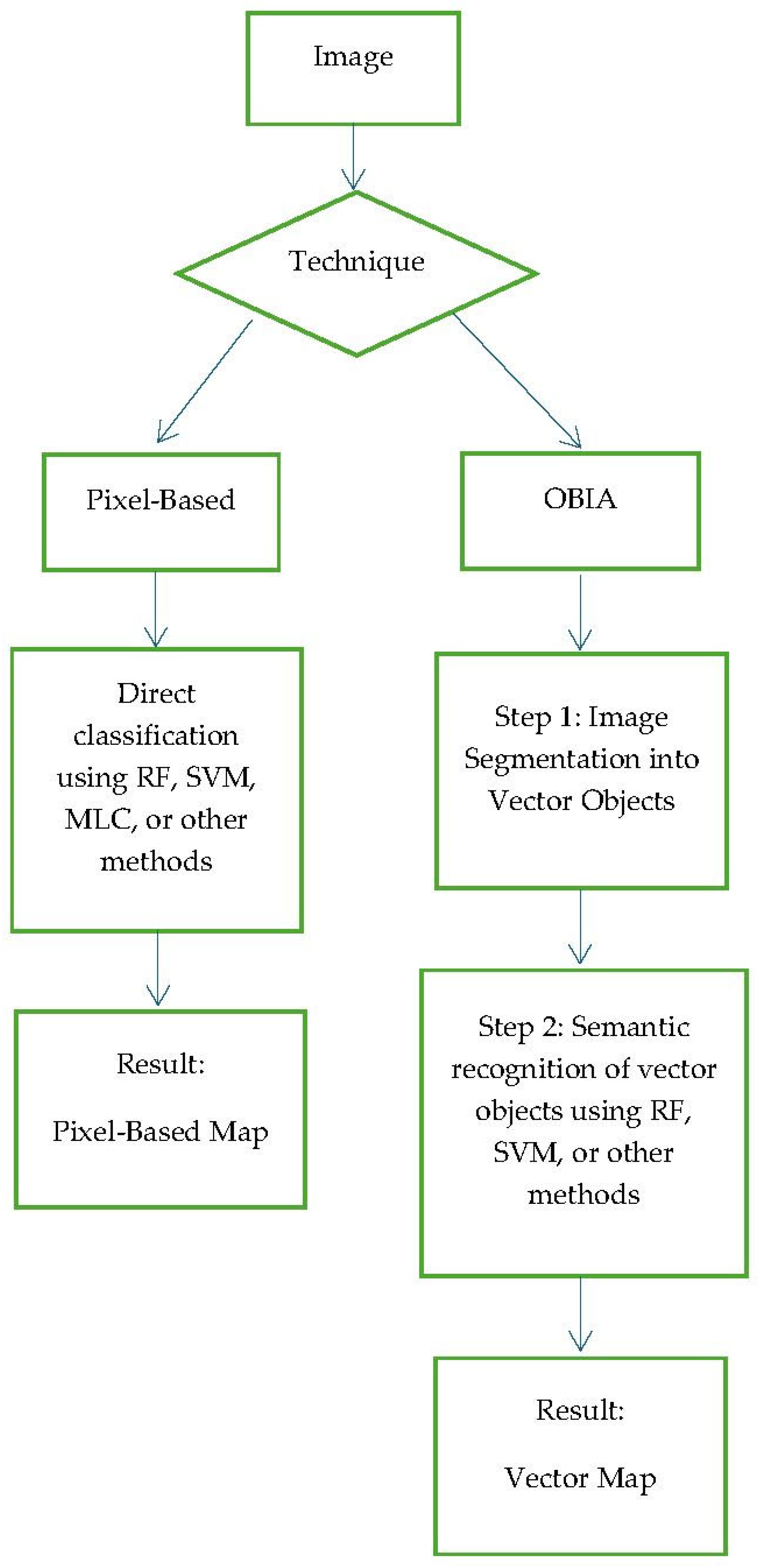
Figure 2.
Classification and illustration of image segmentation algorithm families.
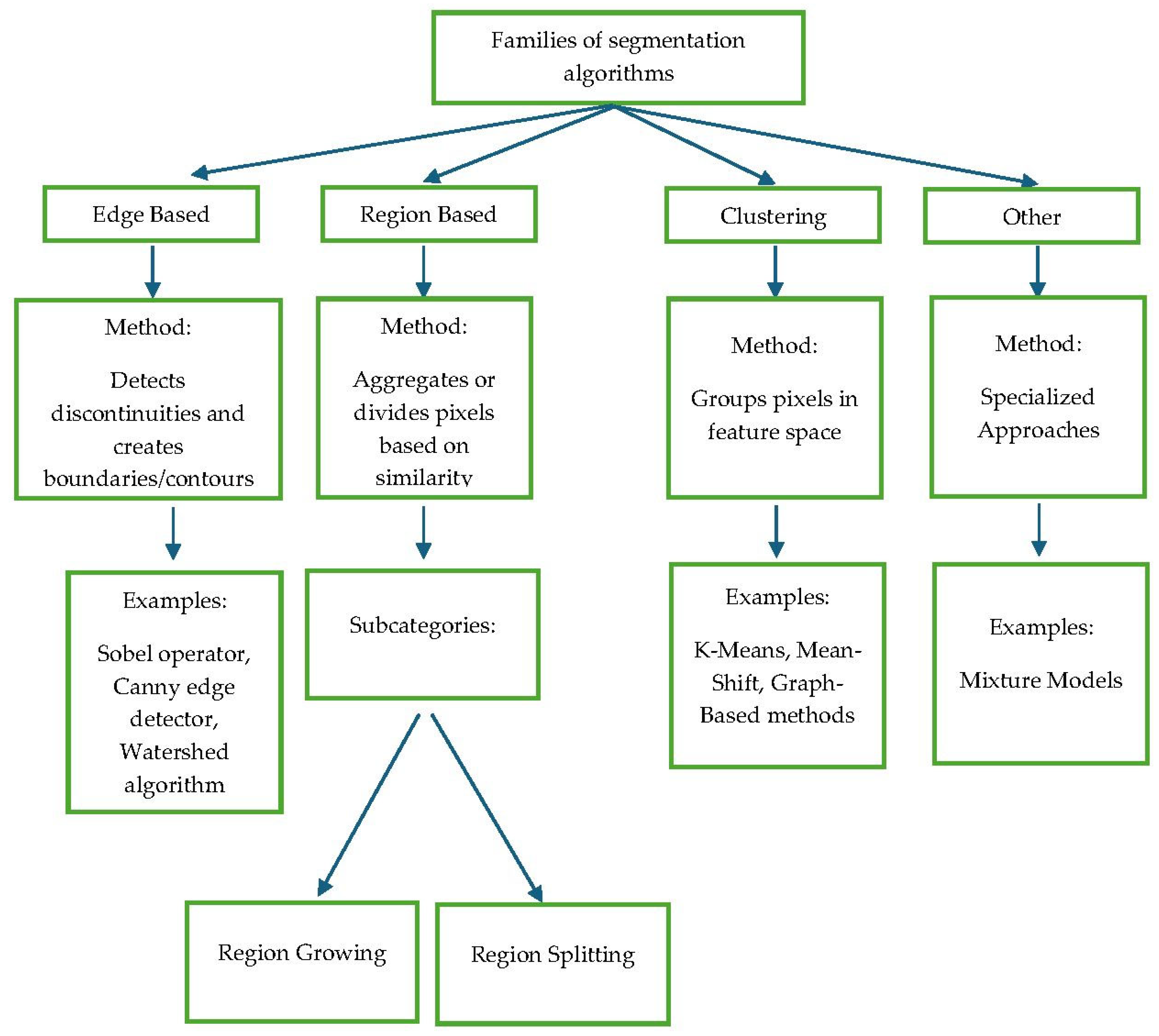
Figure 3.
Ambrosio-Tortorelli Execution Algorithm.
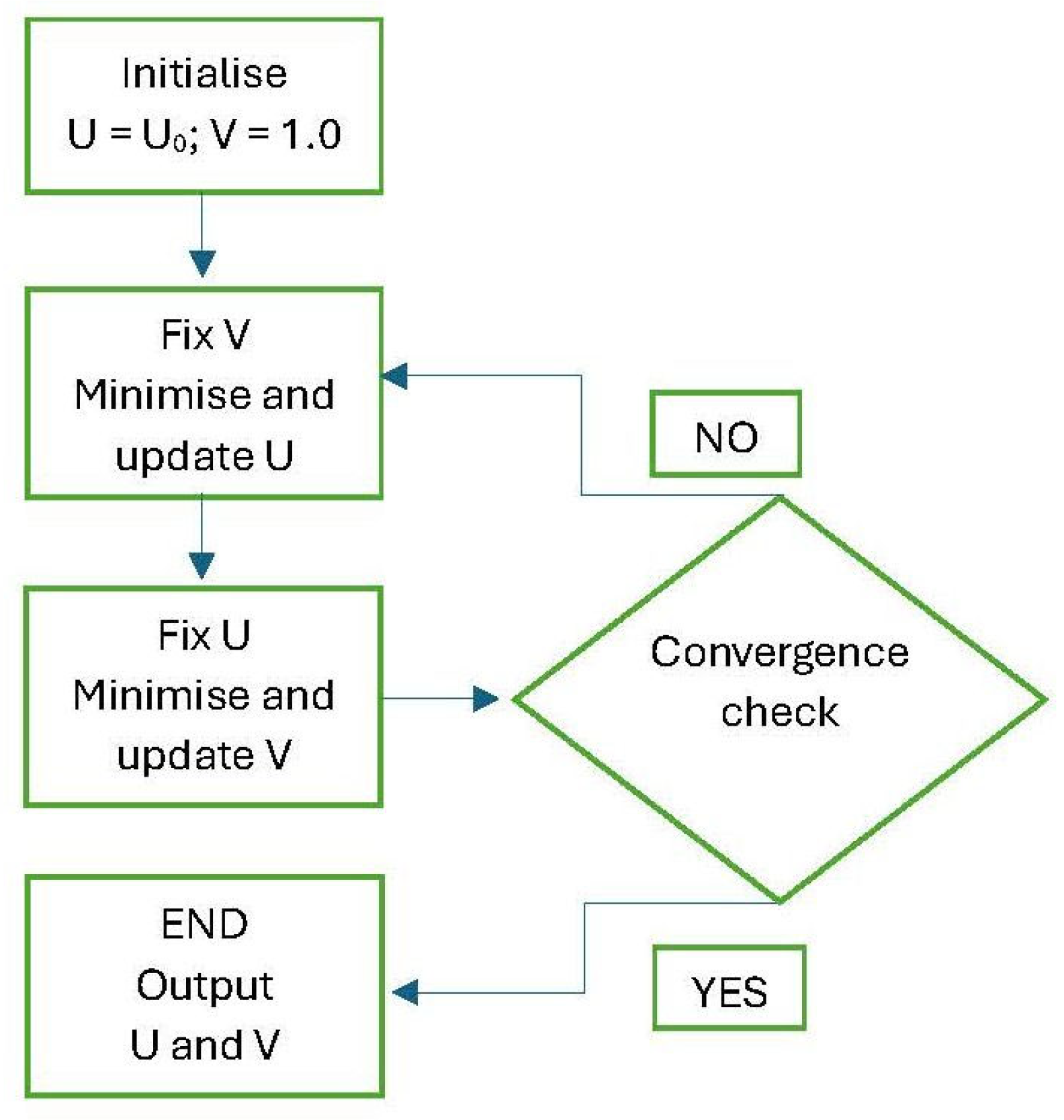
Figure 4.
Vector base image used for testing. Processing by the Authors.
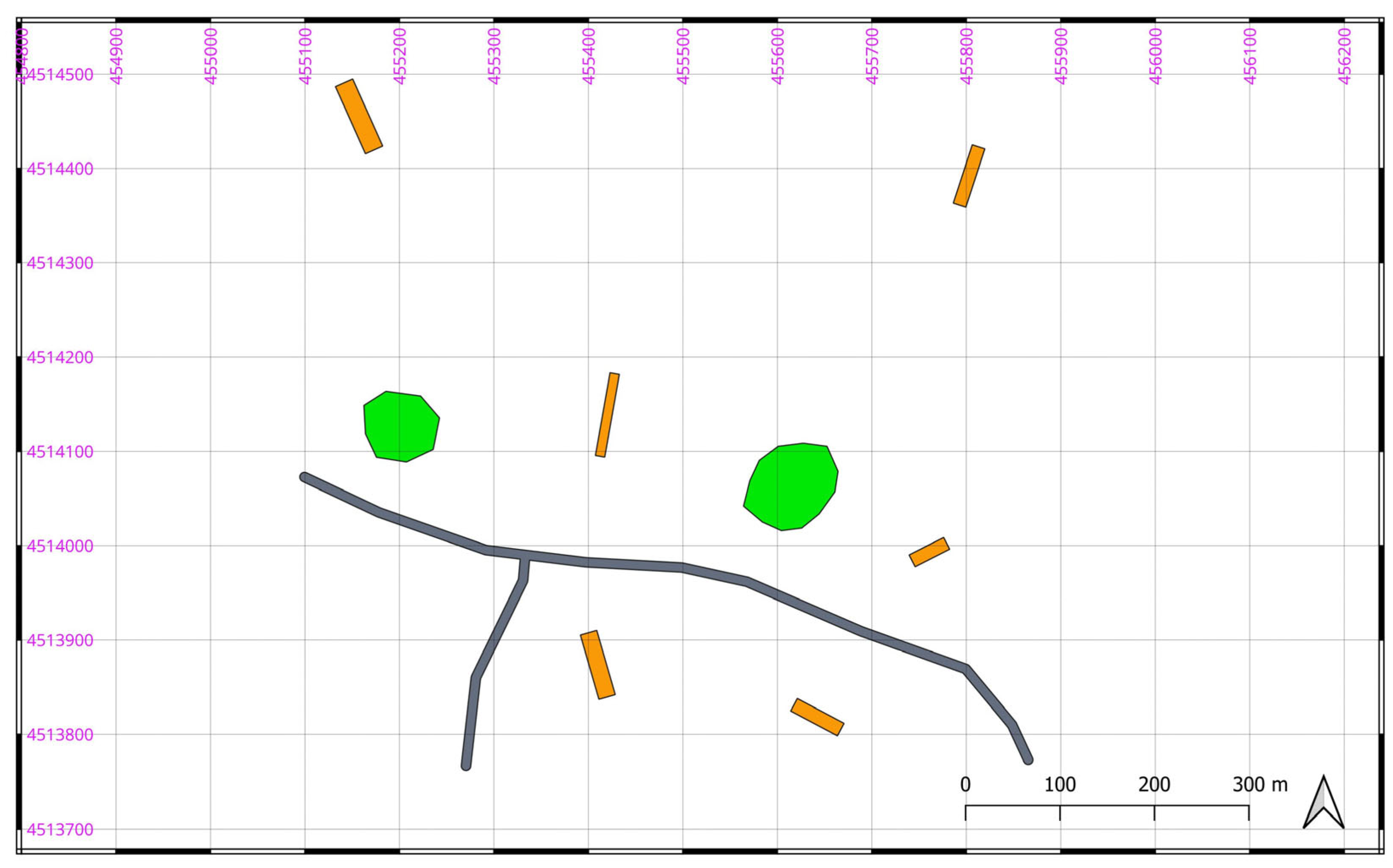
Figure 7.
Left: the original raster image for scenario S_1. Right: the image reconstructed using the Ambrosio-Tortorelli model, showing the determination of edges and the pixels internal to the objects. Processing by the Authors.
Figure 7.
Left: the original raster image for scenario S_1. Right: the image reconstructed using the Ambrosio-Tortorelli model, showing the determination of edges and the pixels internal to the objects. Processing by the Authors.
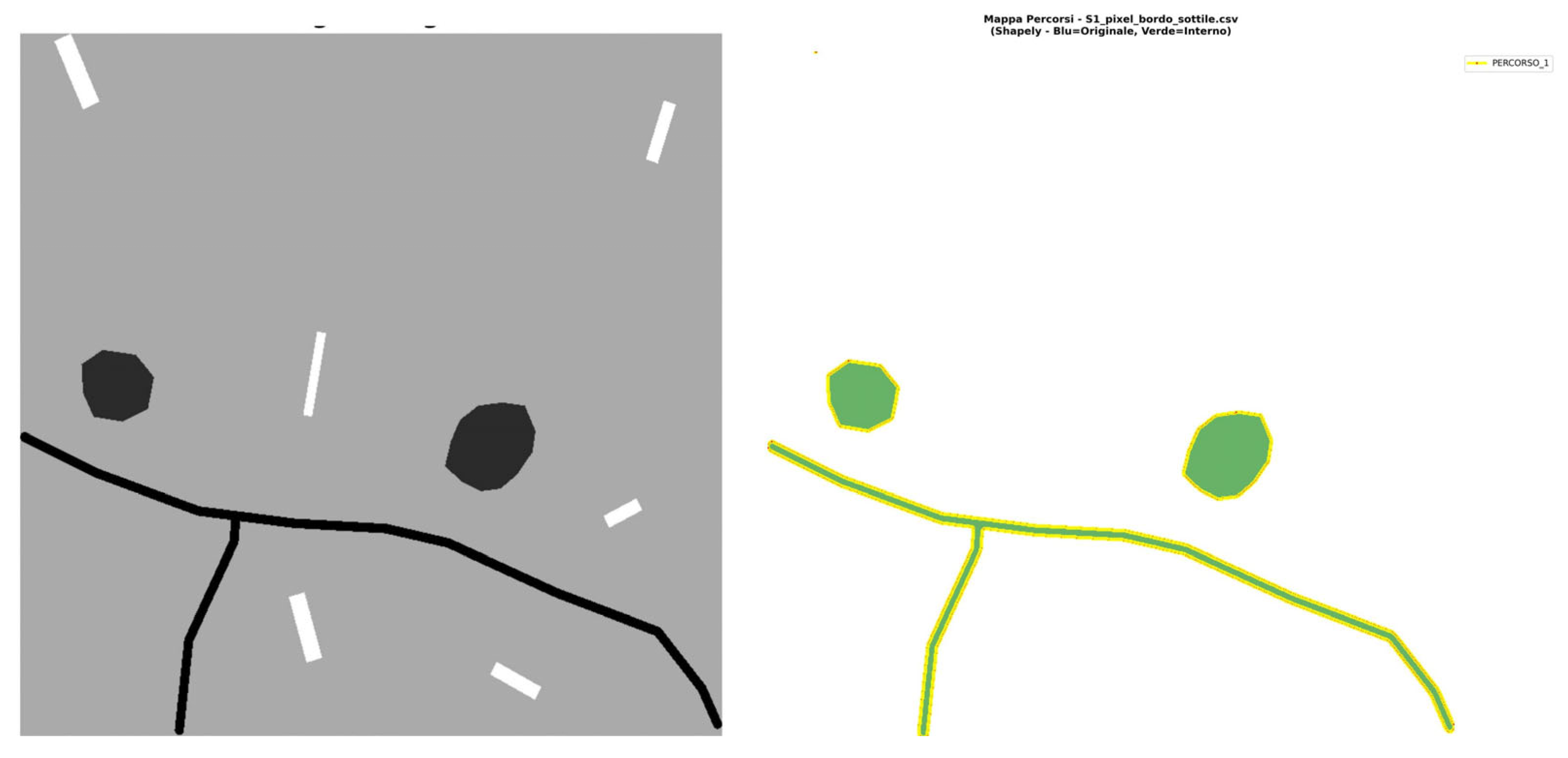
Figure 8.
Left: the original raster image for scenario S1R. Right: the image reconstructed using the Ambrosio-Tortorelli model, showing the determination of edges and the pixels internal to the objects. Processing by the Authors.
Figure 8.
Left: the original raster image for scenario S1R. Right: the image reconstructed using the Ambrosio-Tortorelli model, showing the determination of edges and the pixels internal to the objects. Processing by the Authors.
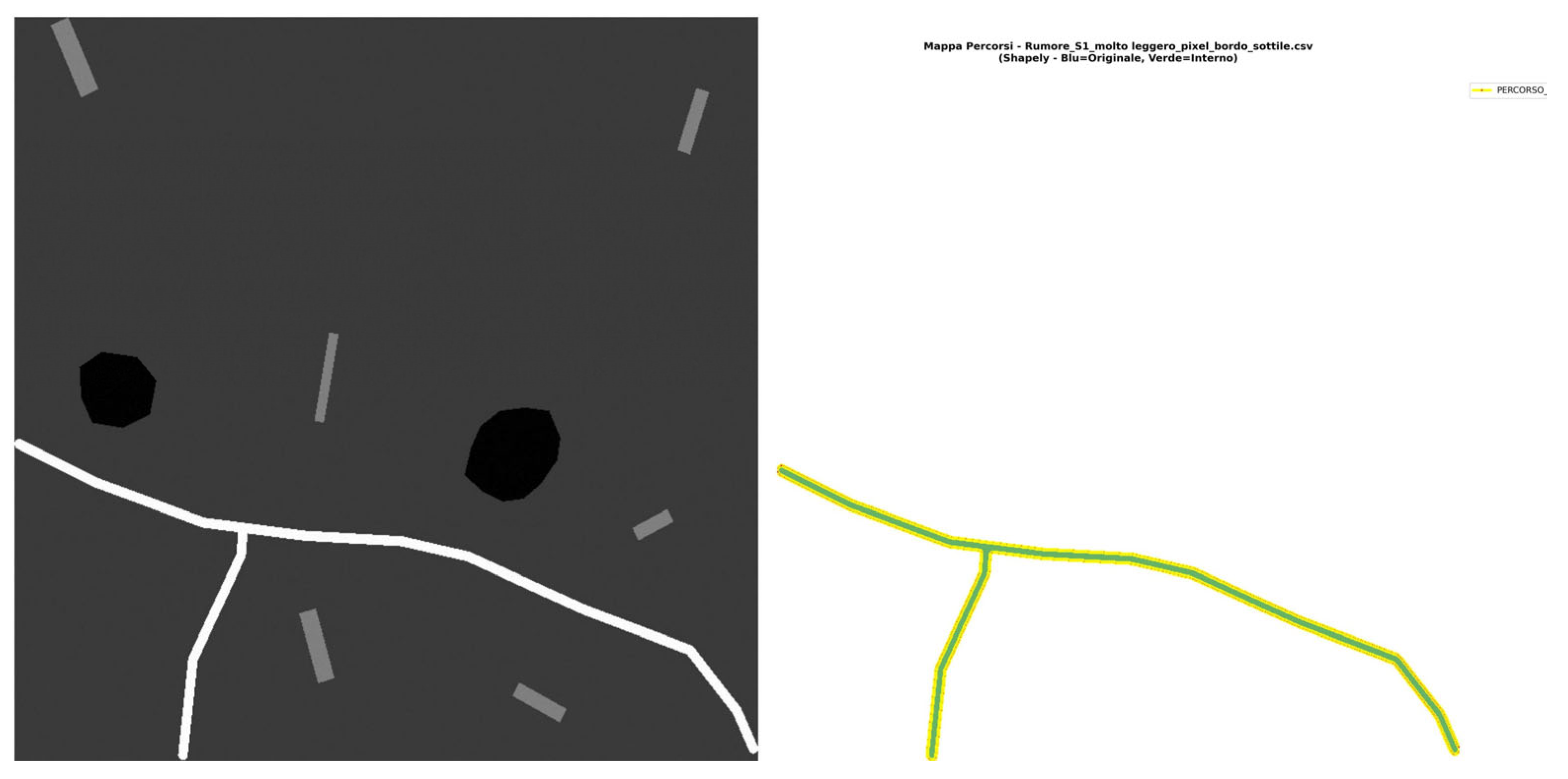
Figure 9.
Left: the original raster image for scenario S1R. Right: the image reconstructed using the Snake model, showing the determination of edges and the pixels internal to the objects. Processing by the Authors.
Figure 9.
Left: the original raster image for scenario S1R. Right: the image reconstructed using the Snake model, showing the determination of edges and the pixels internal to the objects. Processing by the Authors.
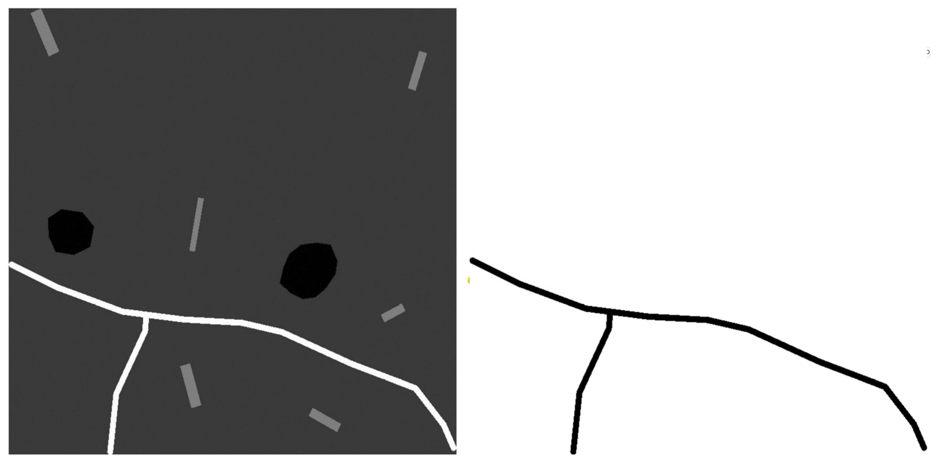
Figure 10.
Left: the original raster image for scenario S4_R. Right: the image reconstructed using the Snake model, showing the determination of edges and the pixels internal to the objects. Processing by the Authors.
Figure 10.
Left: the original raster image for scenario S4_R. Right: the image reconstructed using the Snake model, showing the determination of edges and the pixels internal to the objects. Processing by the Authors.
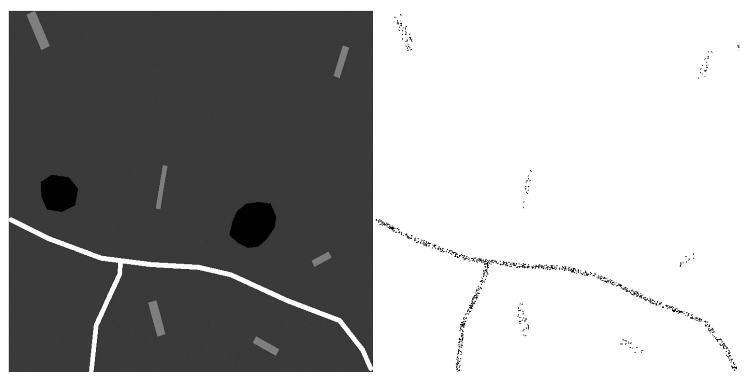
Table 1.
A classification of algorithms according to Supervised versus Unsupervised and Parametric versus Non-parametric methodologies.
Table 1.
A classification of algorithms according to Supervised versus Unsupervised and Parametric versus Non-parametric methodologies.
| Parametric | Non-parametric | |
| Supervised | Maximum Likelihood Classifier (MLC); Regressione Logistica |
Random Forest (RF) Support Vector Machine (SVM) K-Nearest Neighbours (KNN) Neural Networks (ANN) |
| Unsupervised | Gaussian Mixture Models (GMM) | K-Means ISODATA DBSCAN Hierarchical Clustering |
Table 2.
Table summarizing the role of each parameter and suggested “reasonable” initial values.
| Parameter | Interpretation | Range | Parameter Selection Criteria |
| μ | It controls the “importance” or weighting of the regularization on u. | 1 | It is typically set to 1.0 to normalize the other parameters. |
| ν | It controls the “importance” or weighting of the regularization on v (and consequently, of the contour length). | 10-100 | It depends on the scale of the image pixel values. For images in the range [0,255], a value between 20 and 100 serves as a practical starting point. |
| ε | It controls the “width” of the transition of function v from 0 to 1. A smaller ε results in sharper transitions. | 0.1-1.0 | It depends on the scale of the features one aims to capture. A value of 0.5 or 1.0 is often used as an initial estimate. |
Table 3.
Guidance for Setting the Alpha Parameter.
| Alfa value | The effect on the Snake’s behaviour | Analogy |
| 1.0 | Very RIGID Snake, equidistant points | Taut string / cable – does not bend easily |
| 0.4 | Elastic snake, adapts to contours | Elastic band – stretches but retains its form |
| 0.1 | Highly FLEXIBLE snake, irregular points | Slack rope – deforms easily |
Table 4.
Guidance for Setting the Beta Parameter.
| Beta value | The effect on the Snake’s behaviour | Analogy |
| 0.5 | Very smooth snake, fewer details | Train rail – very broad/sweeping curves |
| 0.2 | Balanced snake, good detail | Flexible hose – natural curves |
| 0.05 | Highly jagged snake, very detailed | Wool thread – follows every irregularity |
Table 7.
Results of Cohen’s Kappa and the Jaccard Index from comparing the outputs of the Ambrosio-Tortorelli model and the Snake algorithm against the 10 scenarios without intra-object noise.
Table 7.
Results of Cohen’s Kappa and the Jaccard Index from comparing the outputs of the Ambrosio-Tortorelli model and the Snake algorithm against the 10 scenarios without intra-object noise.
| Ambrosio-Tortorelli | Snake | |||
| Scenario (S) | Cohen’s | Jaccard | Cohen’s | Jaccard |
| S1 | 0.8502 | 0.7498 | 0.0000 | 0.0500 |
| S2 | 0.9657 | 0.9371 | 1.0000 | 1.0000 |
| S3 | 0.9657 | 0.9371 | 1.0000 | 1.0000 |
| S4 | 0.9657 | 0.9371 | 1.0000 | 1.0000 |
| S5 | 0.9657 | 0.9371 | 1.0000 | 1.0000 |
| S6 | 0.9657 | 0.9371 | 1.0000 | 1.0000 |
| S7 | 0.9657 | 0.9371 | 1.0000 | 1.0000 |
| S8 | 0.9657 | 0.9371 | 1.0000 | 1.0000 |
| S9 | 0.9657 | 0.9371 | 1.0000 | 1.0000 |
| S10 | 0.9657 | 0.9371 | 1.0000 | 1.0000 |
Table 8.
Details of the cell-by-cell agreement for “1” and “0” values, comparing the outputs of the Ambrosio-Tortorelli model and the Snake algorithm against the 10 scenarios withoutintra-object noise.
Table 8.
Details of the cell-by-cell agreement for “1” and “0” values, comparing the outputs of the Ambrosio-Tortorelli model and the Snake algorithm against the 10 scenarios withoutintra-object noise.
| Ambrosio-Tortorelli | Snake | |||
| Scenario (S) | Agreement for ‘1’ | Agreement for ‘0’ |
Agreement for ‘1’ | Agreement for ‘0’ |
| S1 | 78.30% | 99.77% | 100% | 0.00% |
| S2 | 99.29% | 99.69% | 100.00% | 100.00% |
| S3 | 99.29% | 99.69% | 100.00% | 100.00% |
| S4 | 99.29% | 99.69% | 100.00% | 100.00% |
| S5 | 99.29% | 99.69% | 100.00% | 100.00% |
| S6 | 99.29% | 99.69% | 100.00% | 100.00% |
| S7 | 99.29% | 99.69% | 100.00% | 100.00% |
| S8 | 99.29% | 99.69% | 100.00% | 100.00% |
| S9 | 99.29% | 99.69% | 100.00% | 100.00% |
| S10 | 99.29% | 99.69% | 100.00% | 100.00% |
Table 9.
Results of Cohen’s Kappa and the Jaccard Index from comparing the outputs of the Ambrosio-Tortorelli model and the Snake algorithm against the 9 scenarios with intra-object noise.
Table 9.
Results of Cohen’s Kappa and the Jaccard Index from comparing the outputs of the Ambrosio-Tortorelli model and the Snake algorithm against the 9 scenarios with intra-object noise.
| Ambrosio-Tortorelli | Snake | |||
| Scenario (S) | Cohen’s | Jaccard | Cohen’s | Jaccard |
| S1_R | 0.5255 | 0.3694 | 0.5431 | 0.3848 |
| S2_R | 0.5255 | 0.3694 | 0.4810 | 0.3279 |
| S3_R | 0.5255 | 0.3694 | 0.4178 | 0.2742 |
| S4_R | 0.5255 | 0.3694 | 0.2410 | 0.1432 |
| S5_R | 0.0617 | 0.0351 | 0.1209 | 0.0675 |
| S6_R | 0.5255 | 0.3694 | 0.4567 | 0.3068 |
| S7_R | 0.5255 | 0.3694 | 0.4189 | 0.2750 |
| S8_R | 0.5255 | 0.3694 | 0.4500 | 0.3010 |
| S9_R | 0.5253 | 0.3992 | 0.1724 | 0.0988 |
Table 10.
Details of the cell-by-cell agreement for “1” and “0” values, comparing the outputs of the Ambrosio-Tortorelli model and the Snake algorithm against the 9 scenarios with intra-object noise.
Table 10.
Details of the cell-by-cell agreement for “1” and “0” values, comparing the outputs of the Ambrosio-Tortorelli model and the Snake algorithm against the 9 scenarios with intra-object noise.
| Ambrosio-Tortorelli | Snake | |||
| Scenario (S) | Agreement for ‘1’ | Agreement for ‘0’ |
Agreement for ‘1’ | Agreement for ‘0’ |
| S1_R | 38.24% | 99.81% | 38.48% | 100.00% |
| S2_R | 38.24% | 99.81% | 32.79% | 100.00% |
| S3_R | 38.24% | 99.81% | 27.42% | 100.00% |
| S4_R | 38.24% | 99.81% | 14.32% | 100.00% |
| S5_R | 3.63% | 99.82% | 6.75% | 100.00% |
| S6_R | 38.24% | 99.81% | 30.68% | 100.00% |
| S7_R | 38.24% | 99.81% | 27.50% | 100.00% |
| S8_R | 38.24% | 99.81% | 30.10% | 100.00% |
| S9_R | 38.23% | 99.81% | 9.88% | 100.00% |
Disclaimer/Publisher’s Note: The statements, opinions and data contained in all publications are solely those of the individual author(s) and contributor(s) and not of MDPI and/or the editor(s). MDPI and/or the editor(s) disclaim responsibility for any injury to people or property resulting from any ideas, methods, instructions or products referred to in the content. |
© 2025 by the authors. Licensee MDPI, Basel, Switzerland. This article is an open access article distributed under the terms and conditions of the Creative Commons Attribution (CC BY) license.
Copyright: This open access article is published under a Creative Commons CC BY 4.0 license, which permit the free download, distribution, and reuse, provided that the author and preprint are cited in any reuse.


