
Submitted:
19 January 2026
Posted:
20 January 2026
You are already at the latest version
Abstract
In this paper, we explore the feasibility of deriving a simple, physically meaningful, andcompact formulation for the pressure distribution and lift of an asymmetric delta wing athigh angles of attack with an attached shock wave. Such a model would be valuable forrapid engineering analysis. Our approach begins with a compact pressure approximationin the linear regime, which is then extended to the nonlinear case through a geometrictransformation and the assumption of functional similarity between linear and nonlinearsolutions. This method bridges the solution in the central nonuniform flow region tothe exact solutions in the uniform flow regions near the leading-edge shock waves , in amanner analogous to methods used for supersonic starting flow. The model is shown to reproduce existing results for both symmetric and yawed delta wings within an acceptable error margin, providing a compact explicit expression for the normal force coefficient as a weighted average of pressure coefficients from the two uniform flow regions. Additionally, weoutline how the approach may be extended to the upper surface, where the uniform flowis described by swept Prandtl-Meyer relations.
Keywords:
asymmetric delta wing
; geometric similarity
; pressure
; lift
; shock wave
1. Introduction
Linear solution for supersonic flow around delta wings has been obtained in the 1940s and 1950s. For instance, Jones (1946), based on slender-body assumptions, proposed a lift theory for low-aspect-ratio pointed wings, indicating that the spanwise loading distribution is elliptical and that lift varies little between subsonic and supersonic speeds. Stewart (1946) employed conical flow theory and conformal mapping to solve the lift problem of delta wings at supersonic speeds, providing an analytical expression for the lift-curve slope and distinguishing between cases where the leading edge lies inside or outside the Mach cone. Puckett (1946) used a source-distribution method to calculate the pressure coefficient of symmetric delta wings and obtained explicit formulas for the pressure coefficients in the two-dimensional and three-dimensional regions, and showed that the lift coefficient is equal to that of a two-dimensional wing, known from Ackeret (1925). Goodman (1949) introduced a method for determining pressure distributions by canceling excess lift, applicable to both conical and non-conical flow regions, illustrated with examples such as rectangular wing tips and clipped delta wings. Malvestuto et al. (1950), based on linearized supersonic-flow theory, derived the lift and damping-in-roll derivatives for sweptback wings with streamwise tips and provided design curves.
For the problem of supersonic/hypersonic flow with attached shock waves over the lower surface of delta wings, particularly under conditions of significant sweep angle and angle of attack where linear theory fails, several theoretical approaches have been developed. These methods crucially employ the exact oblique shock relations to define the uniform flow near the leading edges (Babaev, 1963). The central non-uniform flow region is then addressed using distinct methodologies: the thin shock-layer approximation, which leads to solutions constructed from discontinuous shock slopes (Messiter, 1963; Woods and McIntosh, 1977); the method of integral relations, which reduces the governing equations to ordinary differential equations (Akinrelere, 1970); and a unified perturbation theory that applies a linearized analysis on a nonlinear base flow and uses a strained coordinate technique for matching (Hui, 1971). Hui (1973) also extended the unified perturbation theory to yawed symmetric wings.
All these approaches fundamentally rely on the application of the shock relations to properly account for the three-dimensional, nonlinear effects of sweep and incidence. Roe (1972) derived an exact expression for the spanwise pressure gradient at the boundary between the uniform and non-uniform flow regions beneath a supersonic delta wings with an attached shock. Fowell (1956) considered both lower and upper surfaces of a delta wing, and his analysis revealed the existence of a critical angle of attack on the expansion surface, beyond which the flow becomes discontinuous, forming a shock structure. The flow past the upper surface of the wing was also investigated by Babaev (1962). Since Bluford (1979), effect of viscosity can be accounted using numerical simulation (1979). In the NASA technical paper by Wood (1988), the aerodynamic characteristics of delta wings at lifting conditions were evaluated for the effects of wing leading-edge sweep, leading-edge bluntness, and wing thickness and camber and then summarized in the form of graphs.
For the flow over delta wings at high angles of attack, the theoretical prediction of surface pressure under asymmetric conditions—whether induced by geometric dissimilarity between the left and right leading edges or by a yawed inflow—presents a significant challenge beyond the scope of classical linear theory. Early nonlinear analyses, such as the unified perturbation theory developed by Hui for yawed symmetric wings (Hui, 1973), provided a rigorous theoretical framework capable of handling the coupled effects of sweep and incidence across supersonic and hypersonic regimes. In his work, the asymmetry originates from the yaw angle of the oncoming stream, and the solution is constructed through a sophisticated perturbation approach combined with the method of strained coordinates to match the non-uniform central flow with the exact uniform flows near the leading edges. While theoretically comprehensive, such methods often result in solutions that are implicit or require considerable computational effort for evaluation, limiting their immediate utility for rapid engineering estimation.
Engineering application usually requires simpler, yet accurate and physically sound methods for predicting the lift and pressure distributions over asymmetric delta wings, particularly at high angles of attack.
Motivated by the need for a simpler yet physically sound predictive tool, this paper proposes a geometric transformation approach for asymmetric delta wings with dissimilar sweep angles and with supersonic upstream flow at a Mach number such that there is an attached shock waves and there are two uniform two-dimensional flow regions enclosing a three-dimensional nonuniform flow region in the middle. The geometric transformation has been used by Bai & Wu (2017) for extension of the linear solution of Heaslet & Lomax (1948) to nonlinear case in application of supersonic starting flow at high angle of attack. The problem treated in this paper is different from Bai & Wu (2017) so the geometric transformation has to be reformulated in a form suited to the problem.
The idea is to transform the linear solution, like that given by Puckett (1946, eq.35) for symmetric delta wings, of asymmetrical delta wings, originally expressed in terms of the spanwise coordinate into a geometrically invariant form, and then replace the pressures coefficients pertinent to the two-dimensional uniform flow region by the attached shock solution. This way gives a very simple formula, physcially releveant formula for both two-dimensional and three-dimensional regions over the asymmetrical delta wing.
The linear pressure expression for asymmetric delta wings is provided in Section 2. The nonlinear extension by geometric transformation is given in Section 3. Section 4 is for comparison with exact solutions, for both symmetric delta wings and asymmetric delta wing. Section 3 and Section 4 treat the lower surface. Section 4 gives the expression for the normal force coefficient. Appendix A provides a possible method to extend the present result to the upper surface of asymmetric delta wing.
2. Linear Solution for Asymmetric Delta Wing
2.1. Asymmetric Delta Wings Configuration
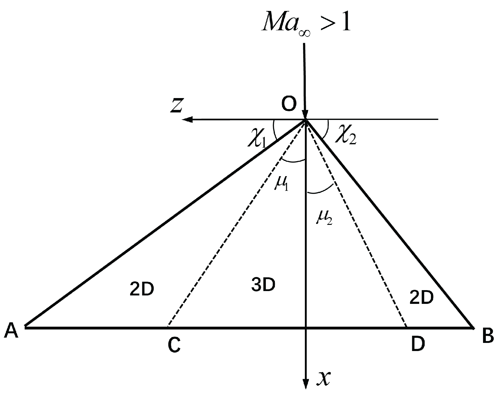
Consider an asymmetric delta wing with different sweep angles (left) and (right). The freestream Mach number is and the angle of attack is (assumed to be small in linear case). See Figure 1 for a schematic display.
The two leading edges, OA and OB, are defined by
Supersonic leading edge conditions are assumed, so
The Mach angle is . As usual, define , so . We also denote
For supersonic leading edges we have and .
The flow region is divided into a two-dimensional (2D) flow region near each leading edge, and a three dimensional (3D) flow region (see Figure 1). The boundaries between 2D and 3D regions, OC and OD, are in fact the Mach waves or boundaries of the Mach cone, i.e.
2.2. Pressure Coefficient Expression
For the left 2D region ( and ), the pressure coefficient is given by Ackeret (1925) solution when swept effect is accounted for
Similarly, for the right 2D region ( and ), the pressure coefficient is given by
The flow in the three-dimensional (3D) flow region (inside the Mach cone from point O, i.e. ) is conical and the pressure coefficient is function of
with for left Mach wave (OC) and for right Mach wave (OD).
We will see below that the pressure coefficient at point in the three-dimensional region can be expressed as
where and satisfy and to ensure that (4) reduces to the two-dimensional solutions at .
The expressions for and can be obtained following the linear supersonic flow theory of Puckett (1946). At point in the three-dimensional region as shown in Figure 1, is given by
where is the upstream region bounded by the Mach cone from P and the two wing leading edges.
The linear pressure expression (5) is solved using a technique proposed by Puckett (1946). This technique consists to decompose (5) into
where the first term on the right hand side is a two-dimensional flow solution and the second term (integral) is defined over the fictif trangle , formed by points O, R and Q, where Q is the intersection of the left leading edge and the extended line of PR (see Figure 1). The expression for can be evaluated using the formula
and
with
Consider a symmetrical delta wings with on both leading edges, we have, according to Puckett (1946)
where .
Now consider a symmetrical delta wings with on both leading edges, we have, according to Puckett (1946)
where .
One would expect that can be obtained by adding the pressure coeffcient for a symmetrical delat wing with and the half of the difference . This would give
The formula (4) with and given by (13) reduces to the exact solution of Puckett (1946) for a symmetric delta wing
However, it can be shown that, at the 2D/3D edges (), (13) does not brigde continuously with the 2D solutions (1) and (2).
To ensure continuity at the edges, a simple way is to modify (13) as
3. Nonlinear Approximation by Geometric Transformation
In the nonlinear extension, we consider inviscid flow and focus on lower-surface with an attached shock wave.
3.1. Geometrical Relations
In nonlinear case, the shock wave depends not on the upstream Mach number, but also on the angle of attack and the leading edge sweep angle. There are two equivalent ways to define the angle of attack and the sweep angle, as shown in Figure 2 and Figure 3.
The configuration shown in Figure 2 was adopted by some authors like Babaev (1963) and Hui (1971). Here, the free stream velocity passing throgh the apex (o) lies on the same plane of the x axis. The y axis is perpendicular to the wing, and z axis is along the span. The wing is on the plane with . The angle of attack is the angle between the free stream and the x axis. The sweep is defined as the sweep in the wing surface, i.e., in plane, thus the sweep angle is defined as the angle between the leading edge and the spanwise axis (z).
In the present case, the left leading edge sweep angle is different from the right leading edge sweep angle . Now consider the left leading edge.
Emanuel (2000) and Domel (2016) considered the shock wave produced by an infinite span sweep wing. The sweep angle is defined as the the sweep in the shock plane as shown in Figure 3, so
and the angle of attack is defined in the plane normal to the leading edge, so
according to Babaev (1963) and Hui (1971).
The angle between the free stream velocity and the leading edge is denoted as . According to Hui (1971),
3.2. Shock Solution in the Two-Dimensional or Uniform Region
Numerous authors have given the expressions for shock solutions accouting for the swept angle effect of the leading edge (e.g. Babaev 1963; Akinrelere 1970; Hui, 1971; Emanuel 2000;Threadgill & Little 2020). As noted by Hui (1971), the flow field on the lower surface of a delta wing consists of uniform flow regions near the leading edges, where the cross flow is supersonic and a nonuniform flow region near the central part. Now we provide the shock expressions for the uniform region.
The Domel’s 3-D theta-beta–Mach-sweep () shock relations are written in a form very similar to the two-dimensional counterpart and easy to use here. As commented by Threadgill & Little (2020), Domel (2016)’s theta-beta–Mach-sweep shock relations have been derived for infinite-span swept oblique inviscid shock. However, the uniform flow region of the delta wings can be described by the infinite-span swept oblique shock relations.
Note that the sweep angle and the angle of attack in the Domel’s definitions are related to those in the definitions of Babaev (1963) and Hui (1971) by (16) and (17).
Domel discovered the existence of an effective 2-D plane that can be obtained by rotation of his y plane (this y is the axis normal to the shock surface) by a tilt angle () and on this effective plane he introduced the effective deflection angle and the effective shock angle . First, the effective shock angle is solved by
and then the effective deflection angle is solved by
Once is obtained by (18) and is obtained by (19), the Mach number M, the pressure p and the density downstream of the shock wave are computed by
Using (21), the pressure coefficient is
3.3. Geometric Transformation
To extend the linear expression to nonlinear cases directly, we need a geometrical transformation. Bai & Wu (2017) proposed such a method when extending the Heaslet & Lomax (1948) linear solution for starting flow at small angle of attack to nonlinear case at large angle of attack. This geometric transformation is used to make the linear expression in a form that is invariant to frame rotation and nonlinear extension.
To write the geometrical transformation in a more convenient way, the positions of the left boundary and right boundaries of the wing are denoted as
and the positions of the left boundary and right boundaries of the Mach cone from the apex (O) are denoted as
3.4. Nonlinear Solution for the Three Dimensional Region
In the nonlinear case, the left and right boundaries of the wing are still given by (24), the left and right boundaries of the Mach cone, or the edges between the two-dimensional regions and three dimensional region, are no longer given by (25), but are given by
where and , is the Mach numbers in the left two dimensional flow region downstream the shock wave, and is the Mach numbers in the right two dimensional flow region downstream the shock wave.
4. Comparison with Exact Method
4.1. Symmetric Delta Wing
Babaev (1963), Kutler & Lomax (1971), Bluford (1979), Woods & McIntosh (1977), Roe (1972) and Woods (1988) provided various cases which can be used to check the approximate yet very simple method provided above.
Table 1 displays computed by (18), by (19), by (20) and by (23) for several cases. Consider for instance case 1, Babaev (1963) and Hui (1971) gives which is the same as given by Domel’s shock expressions.
We check whether the formula (30) predicts correctly the boundaries between the two-dimensional regions and the three-dimensional region, for symmetric case as shown in Table 1. In symmeric case, we consider just the right boundary defined by
where , with given by (20). The value is from Babaev (1963) for case 1, Woods & McIntosh (1977) for case 2 and 3, from Babaev (1963) (see also Roe 1972) for case 3, from Babaev (1963) and Squire (1968) for case 4 ( is from Babaev 1963 and is from Squire 1968). The relative difference is also shown in Table 2. Thus, there is some discrepancy between predicted by (32) and provided by various previous works.
Now we check whether the formula (31) can predict the previous results for test cases shown in Table 1. In symmetric case, the minimal value of is given by
where is given by (23), and .
The results are shown in Table 3, where is from Babaev (1963) for case 1, Woods & McIntosh (1977) for case 2, from Babaev (1963) (see also Roe 1972) for case 3, from Babaev (1963) and Squire (1968) for case 4 ( is from Babaev 1963 and is from Squire 1968). The relative difference is also shown in Table 1. Thus, the very simple and easy to use formula can predict the minimum pressure coefficient within a difference at most compared to very complex accurate results.
4.2. Yawed Delta Wing
Hui (1973) extended his method for symmetric delta wings (Hui 1971) to the case with yawed delta wing. He provided results that appear to match the present asymmetric delta wings.
For and , Hui (1973) considered yawed delta wings which corresponds to and . For and , he considered yawed delta wings which corresponds to and . He showed the pressure distribition in their Figure 5 and Figure 6 (we have checked that the conditions marked in their Figure 5 and Figure 6 should be exchanged).
For comparison we use the Domel’s expression for and and the formula (31) for . The comparison is displayed in Table 4, where , and are from Figure 5 and Figure 6 of Hui (1973). Here is obtained from (31) with with given by the expression (15) and is obtained from (31) with given by the expressions (9) and (10).
The pressure distribution of Hui (1973) indicates that the minimum occurs at or . Figure 4 shows the pressure distribution prediced by (31) with given by the expression (15). We see that minimum occurs not at or . Figure 5 shows the pressure distribution prediced by (31) with given by the expressions (9) and (10). We see that minimum occurs at or . Overall the pressure distribution prediced by (31) with given by the expressions (9) and (10) produce well the results of Hui (1973).
Figure 4.
Pressure distribution for the two cases of Hui (1971), with given by (15). a) , , and . b) , , and .
Figure 4.
Pressure distribution for the two cases of Hui (1971), with given by (15). a) , , and . b) , , and .
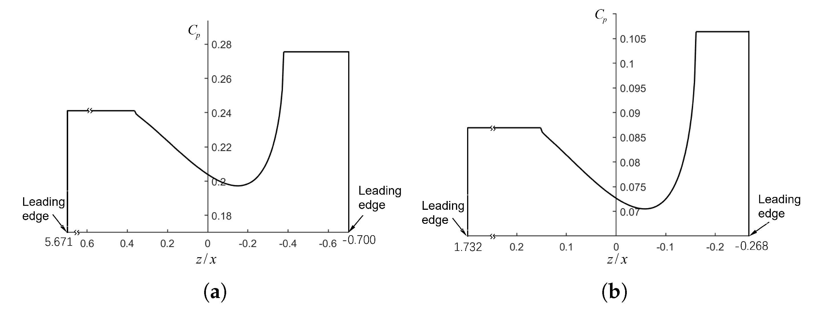
Figure 5.
Pressure distribution for the two cases of Hui (1971), with given by the expressions (9) and (10). a) , , and . b) , , and .
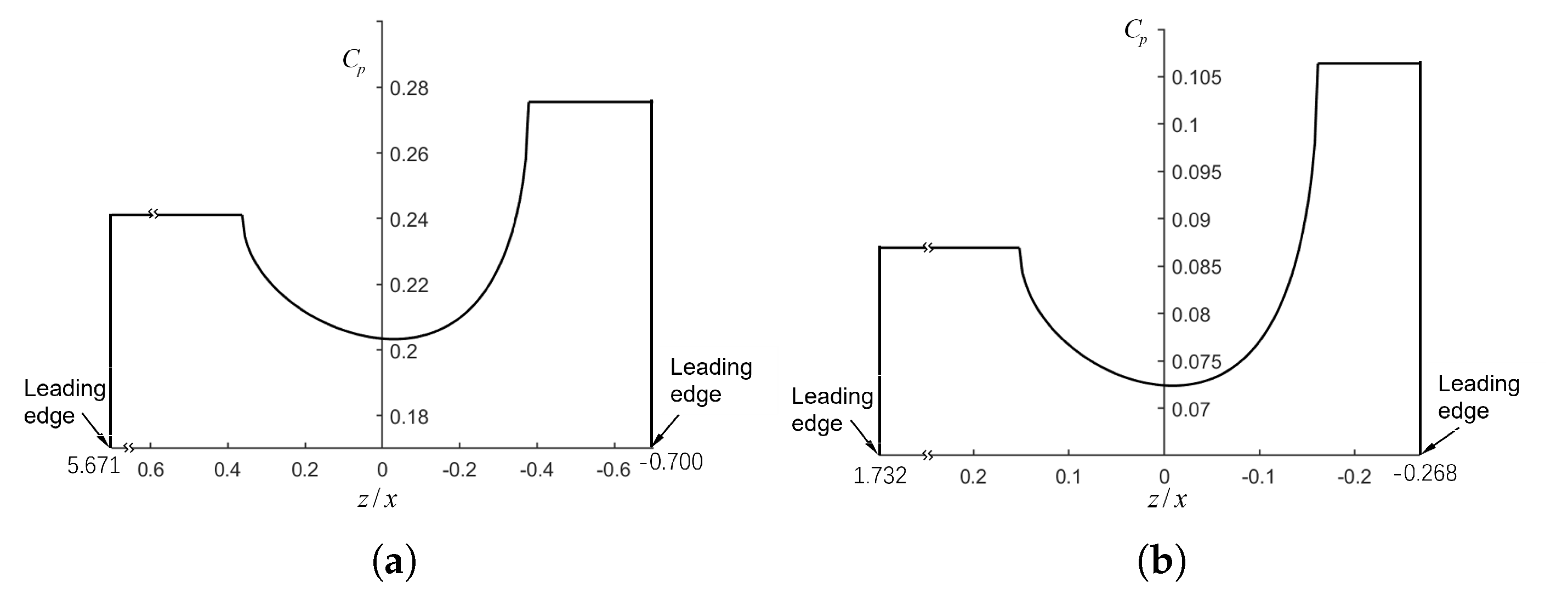
It is interesting to note that, despite the delta wing is highly asymmetric, the centerline of the Mach cone (or position of the minimal value ) coincides almost exactly with the axis in both Hui (1973)’s work and in the present model with given by the expressions (9) and (10).
To consider more quantitative information about asymmetry, we consider and for various . Using Domel’s method, we get and (see Table 1). The asymmetry of the position of can be measured with
where is the middle of the three-dimensional region defined by (29). In the symmetrical case, , so the magnitude of characterize asymmetry of the three-dimensional region.
Table 5 displays , ,, , and for several choices , including the symmetric case . The parameters and are computed by (26) and (27), with and determined by (30), i.e.
The parameter is computed by (33), is computed with the Domel’s formula (23) for , and is computed by (31) with given by (9) and given by (10).

Table 5.
Typical flow parameters for various sweep angle on the right leading edge.
| Case | ||||||
| 1 | 2.8736 | 0.2597 | 0.0000 | 0.1840 | ||
| 2 | 2.8605 | 0.2643 | 0.1822 | |||
| 3 | 2.8418 | 0.2709 | 0.1805 | |||
| 4 | 2.8117 | 0.2817 | 0.1791 | |||
| 5 | 2.7410 | 0.3077 | 0.1795 |
We see that asymmetry parameter is negative, meaning that the middle line of the three dimensional region is one the side with larger sweep angle. The minimum pressure coefficient decreases with increasing . In all cases, the magnitude of is very small, showing that the asymmetry of the delta wings does not change significantly the middle of the three dimensional region.
5. Lift or Normal Coefficient for Asymmetric Delta Wings
The lift is normal to the incoming flow direction, so the lift coefficient where is the normal force coefficient. Here we show that the normal force coefficient due to the pressure of the lower surface of an asymmetric delta wings at high angles of attack can be expressed as a weighted average of the pressure coefficients in the two uniform flow regions near the left and right leading edges.
The schematic display Figure 1 for the linear case is replaced by Figure 6 in nonlinear case. In the latter case, the Mach waves OC and OD are not symmetric with respect to the x axis. Moreover, for , it can be shown that at least for the conditions shown in Table 4.
Figure 6.
Schematic display of a delta wing in nonlinear case.
The normal force coefficient is obtained by integrating the pressure over the wing surface:
where is the reference area of the delta wings, is the aera of the left two-dimensioanl flow region (h is the hight of the delta wing), is the aera of the right two-dimensioanl flow region, and . With the expression (31), we get
where
where and are given by (9) and (10) and is defined by (28).
Define
where and are defined by (30), then and , and using (35), we get from (34) the following compact form for
where
and
Note that () are the pressure coefficients in the two-dimensional uniform flow regions (given by shock relations in Section 3.2), and the weights are functions of and .
For a symmetric delta wings with , we have , , , and Eq. (37) can be shown to give
In the linear limit (small angle of attack and small disturbances), , where . Substituting this into Eq. (40) yields
This is exactly one-half of the lift coefficient given by Puckett (1946) for a symmetric delta wings (which includes both upper and lower surfaces). See also Stewart (1946) for the lift when the leading edge is subsonic. Puckett’s result for the entire wing is ; thus, the present formula correctly recovers the lower-surface contribution in the linear symmetric limit.
6. Conclusions
This paper presents an approximate analytical method based on geometric transformation for predicting the pressure distribution on an asymmetric delta wings with attached shock waves at high angles of attack. By reformulating the linear solution into a geometrically invariant form and replacing the pressure coefficients in the two-dimensional regions with those given by shock relations, a simple algebraic-type formula with clear physical meaning is derived. The core idea is to use geometric transformation as a bridge connecting the nonlinear flow problem to known linear solutions, analogous to the approach used in studies of supersonic starting flow at high incidence. The normal force coefficient is also obtained. The method is validated against existing reference solutions for both symmetric and asymmetric (yawed) delta wings.
The main contribution of this study lies in providing a physically transparent pathway for analyzing asymmetric delta wings under complex conditions. It avoids the substantial computational effort typically required by sophisticated perturbation theories or numerical simulations. The resulting formulas are simple and compact, making them suitable for further extensions that account for viscous effects.
Currently, the method primarily addresses the lower surface. Extension to the upper surface—which involves more complex three-dimensional expansion waves and possible inboard shocks—requires further treatment of intricate wave interactions (a conceptual pathway is outlined in Appendix A, though it remains unvalidated).
Appendix A Possible Extension for the Upper Surface
Despite the linear solution shares the same form on both lower and upper surface, the nonlinear solution on the upper surface is far more complex than on the lower surface. Babaev (1962) pointed out that apart from a three-dimensional Prandtl-Meyer expansion wave, there is also an inboard shock The reason is that, the streams from two halves of the wing having velocity components equal in magnitude but opposite in direction tend to meet on the plane of symmetry of the wing, and a shockwave must arise, on crossing which and behind which the stream changes to a direction parallel to the root chord. Even for the Prandtl-Meyer expansion wave, a numerical integration of the characteristic equation is required to find the flow properties in the uniform flow region. Fowell (1956) studied a plane delta wings with supersonic leading edges, an exact analysis based upon the equations for inviscid flow with constant stagnation enthalpy showed the existence of two cases in the solution of the flow over the expansion surface; below a critical angle of attack a continuous solution can exist while above this angle the solution must be discontinuous.
Using three dimensional method of characteristics, Beeman & Powers (1969) identified four regions of flow on the upper surface. Kutler & Lomax (1971) used computational fluid dynamics to study high angle of attack flow around a delta wing, and noted that Babaev fails to predict the correct values of the flow quantities in the region of uniform flow adjacent to the wing surface and between the inboard shock wave and the wing leading edge..
Bannink & Nebbeling (1973) experimentaly studied the flow around a delta wing, and arrived at the conclusion that the inviscid flowfield at the expansion side of the delta wings appears to be conical and suggested that the inboardshock wave ends with zero strength in the point where the conical sonic line starts.
Neglecting the effect of inboard shock, the present method can be extended to the upper surface in the following way.
First determine the Mach number and pressure coefficients in the two-dimensional uniform region using the Prandtl-Meyer solution of Vahrenkamp (1992) with sweep (), angle of attack () and upstream Mach number () in his M.S. thesis (section 10.3 of Emanuel 2000). This is done for the two-dimensional region along each side of the delta wings, with different sweep angles and
Then, compute the boundaries of the three-dimensional regions by (30), where and , is the Mach numbers in the left two dimensional flow region downstream the Prandtl-Meyer wave, and is the Mach numbers in the right two dimensional flow region downstream the Prandtl Meyer wave.
The pressure coefficient in the three-dimensional region is computed by (31), in the same way as for the lower surface, except that the pressure coefficients are given by the Vahrenkamp’s expression.
Finally, the normal force coefficient due to upper surface is computed by (37), in the same way as for the lower surface, except that , and the pressure coefficients are based on the Vahrenkamp’s expression.
Acknowledgment. The authors are grateful to their comments which help to improve the paper. This work was supported partly by the National Key Project (grant no. GJXM92579).
References
- Ackeret, J. 1925. Air Forces on Airfoils Moving Faster than Sound. Zeitschrift fur Flugtechnik und Motorluftschiffahrt, February 14, 1925, pp. 72–74. (English trans. as NACA Technical Memorandum No. 317, 1935).
- Akinrelere, E. A. 1970. The calculation of inviscid hypersonic flow past the lower surface of a delta wing. Journal of Fluid Mechanics, 44(1), 113–127. [CrossRef]
- Babaev, D. A. 1962. Numerical solution of the problem of supersonic flow past the upper surface of a delta wing. Zhur. Vychisli Tel’noi Matematiki i Matematicheskoi Fiziki (J. Computational Math, and Mathemat. Phys.), 2(2), 278–289. [CrossRef]
- Babaev, D. A. 1963. Numerical solution of the problem of supersonic flow past the lower surface of a delta wing. AIAA Journal, 1(9), 2224–2231. [CrossRef]
- Bai, C. Y., and Wu, Z. N. 2017. Supersonic indicial response with nonlinear corrections by shock and rarefaction waves. AIAA Journal, 55(3), 884–892. [CrossRef]
- Bannink, W. J., and Nebbeling, C. 1973. Investigation of the expansion side of a delta wing at supersonic speed. AIAA Journal, 11(8), 1151–1156. [CrossRef]
- Beeman, E., and Powers, S. 1969. A method for determining the complete flow field around conical wings at supersonic/hypersonic speeds. Paper presented at AIAA Fluid and Plasma Dynamics Conference, San Francisco, California, June 16–18, 1969.
- Bluford, G. S. 1979. Numerical Solution of the Supersonic and Hypersonic Viscous Flow around Thin Delta Wings. AIAA Journal, 17(9), 942–949. [CrossRef]
- Domel, N. D. 2016. General three-dimensional relation for oblique shocks on swept ramps. AIAA Journal, 54(1), 310–319. [CrossRef]
- Emanuel, G. 2000. Analytical Fluid Dynamics, 2nd ed. CRC Press.
- Fowell, L. R. 1956. Exact and Approximate Solutions for the Supersonic Delta Wing. Journal of the Aeronautical Sciences, 23(8), 709–720. [CrossRef]
- Goodman, T. R. 1949. The lift distribution on conical and non-conical flow regions of thin finite wings in a supersonic stream. Journal of the Aeronautical Sciences, 16(6), 365–374. [CrossRef]
- Heaslet, M. A., and Lomax, H. 1948. Two-Dimensional Unsteady Lift Problems in Supersonic Flight, Archiveand Image Library TR 945 Washington, D.C., 1949; also NACA TN-1621, 1948.
- Hui, W. H. 1971. Supersonic and hypersonic flow with attached shock waves over delta wings. Proceedings of the Royal Society of London. Series A, 325(1561), 251–268. [CrossRef]
- Hui, W. H. 1973. Effect of yaw on supersonic and hypersonic flow over delta wings. Aeronautical Journal, 77, 299–301. [CrossRef]
- Jones, R. T. 1946. Properties of Low-Aspect-Ratio Pointed Wings at Speeds Below and Above the Speed of Sound. NACA Report 835.
- Kutler, P., and Lomax, H. 1971. Shock-capturing, finite-difference approach to supersonic flows. Journal of Spacecraft and Rockets, 8(6), 1179–1182. [CrossRef]
- Malvestuto, F. S. Jr., Margolis, K., and Reiner, H. S. 1950. Theoretical lift and damping in roll at supersonic speeds of thin sweptback tapered wings with streamwise tips, subsonic leading edges, and supersonic trailing edges. NACA Report 970.
- Messiter, A. F. 1963. Lift of slender delta wings according to Newtonian theory. AIAA Journal, 1(4), 794–802. [CrossRef]
- Puckett, A. E. 1946. Supersonic Wave Drag of Thin Airfoils. Journal of the Aeronautical Sciences, 13(9), 475–484. [CrossRef]
- Roe, P. L. 1972. A result concerning the supersonic flow below a plane delta wing (CP No. 1228). London: Her Majesty’s Stationery Office.
- Squire, L. C. 1968. Calculated pressure distributions and shock shapes on conical wings with attached shock waves. Aeronautical Quarterly, 19(1), 31–50. [CrossRef]
- Stewart, H. J. 1946. The lift of a delta wing at supersonic speeds. Quarterly of Applied Mathematics, 4(3), 246–254. [CrossRef]
- Threadgill, J. A. S., and Little, J. C. 2020. An inviscid analysis of swept oblique shock reflections. Journal of Fluid Mechanics, 890, A22.
- Vahrenkamp, M. 1992. Prandtl–Meyer Flow with Sweep. M.S. thesis, University of Oklahoma.
- Wood, R. M. 1988. Supersonic Aerodynamics of Delta Wings. NASA TP-2771.
- Woods, B. A., and McIntosh, C. B. G. 1977. Hypersonic flow with attached shock waves over plane delta wings. Journal of Fluid Mechanics, 79(2), 361–377. [CrossRef]
Figure 1.
Schematic display of a delta wing. The coordinate system is defined with x along the chordwise direction, z along the spanwise direction, and y normal to the wing surface.
Figure 1.
Schematic display of a delta wing. The coordinate system is defined with x along the chordwise direction, z along the spanwise direction, and y normal to the wing surface.
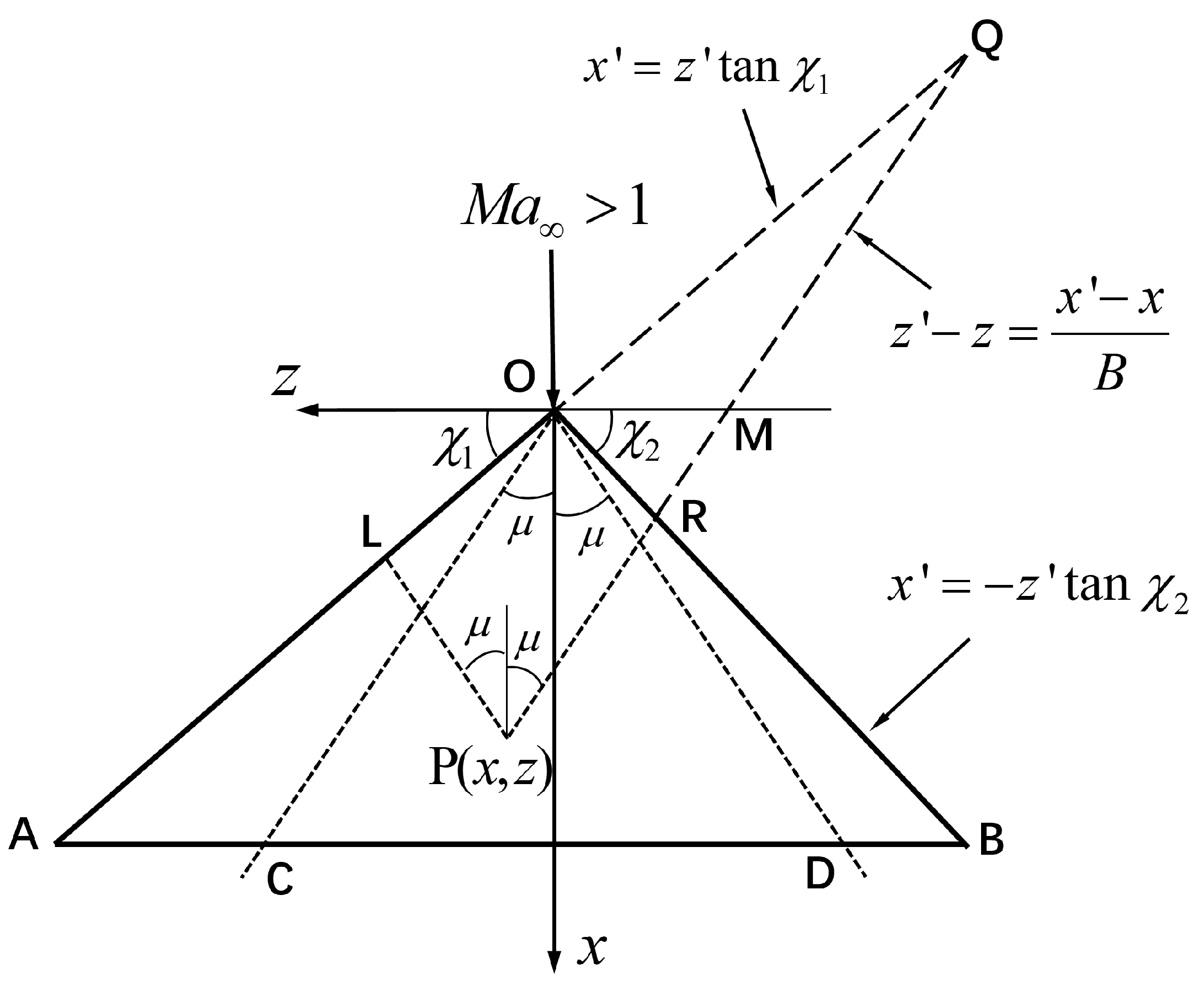
Figure 2.
Schematic display of a delta wing at high angle of attack (following Babaev 1963). The coordinate system is defined with x along the chordwise direction, z along the spanwise direction, and y normal to the wing surface.
Figure 2.
Schematic display of a delta wing at high angle of attack (following Babaev 1963). The coordinate system is defined with x along the chordwise direction, z along the spanwise direction, and y normal to the wing surface.
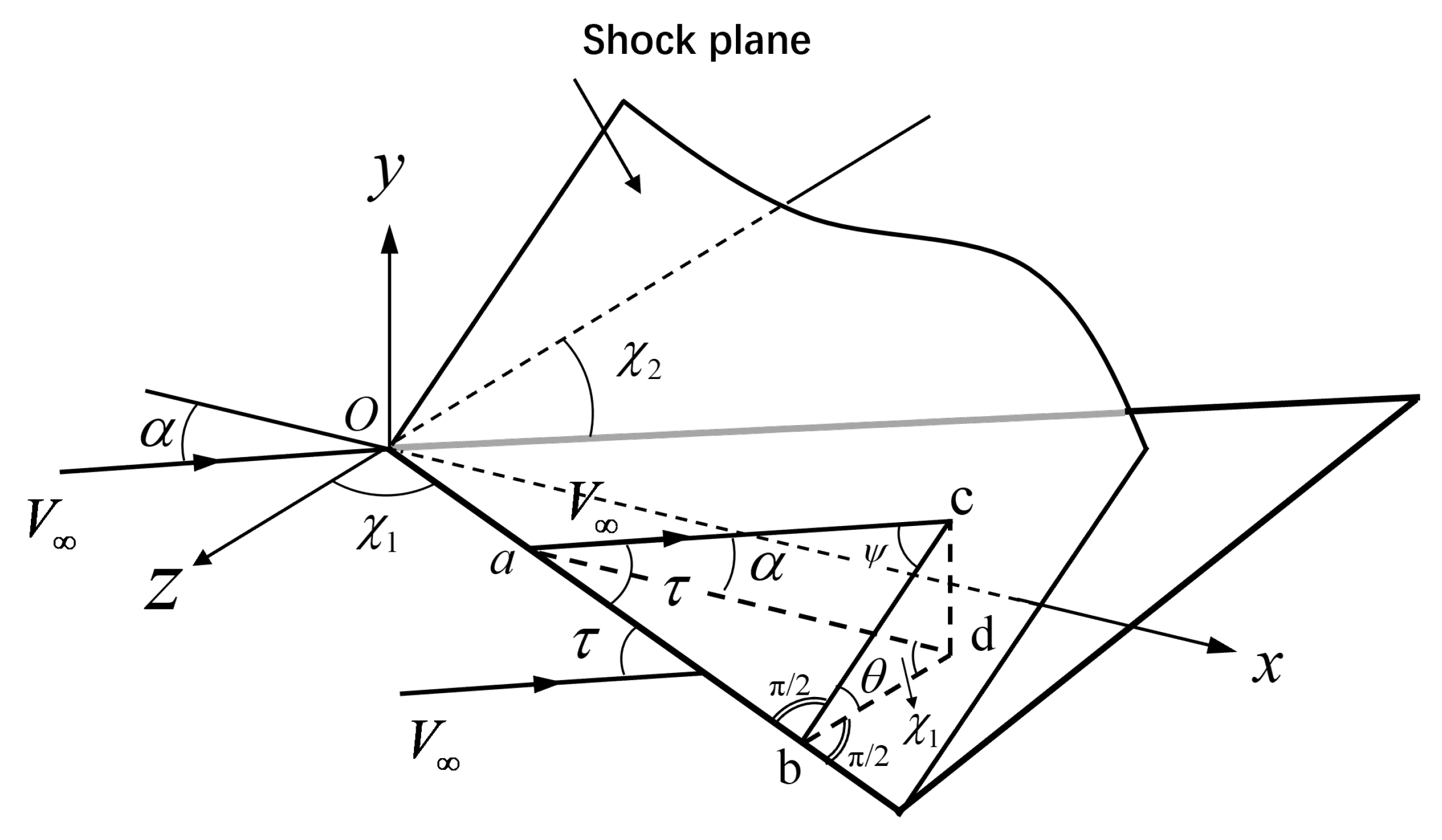
Figure 3.
Top view from the top of the shock surface.
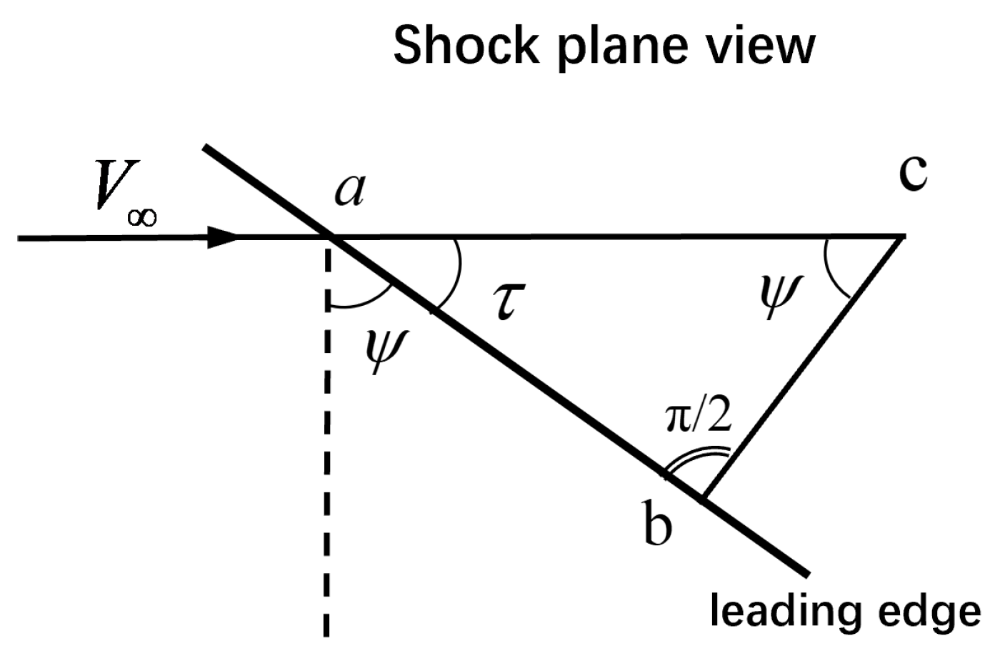
Table 1.
Shock solution for four cases.
| Case | (Domel) | (Domel) | ||||
| 1 | 4.0 | 2.874 | ||||
| 2 | 5.08 | 3.613 | ||||
| 3 | 4 | 2.795 | ||||
| 4 | 6 | 3.207 |
Table 2.
Boundaries between 2d and 3d regions for four cases shown in Table 1.
Table 2.
Boundaries between 2d and 3d regions for four cases shown in Table 1.
| Case | |||||
| 1 | 2.874 | 0.442 | |||
| 2 | 3.613 | 0.343 | |||
| 3 | 2.795 | 0.458 | |||
| 4 | 3.207 | 0.391 |
Table 3.
Minimum pressure coefficients for four cases shown in Table 1.
Table 3.
Minimum pressure coefficients for four cases shown in Table 1.
| Case | ||||
| 1 | 0.184 | |||
| 2 | 0.155 | |||
| 3 | 0.201 | |||
| 4 | 0.276 |
Table 4.
Comparison with the results of Hui (1973).
| Case | |||||||
| 1 | 0.241,0.276 | 0.241,0.278 | 0.203 | 0.197 | |||
| 2 | 0.0869,0.106 | 0.072 | 0.071 |
Disclaimer/Publisher’s Note: The statements, opinions and data contained in all publications are solely those of the individual author(s) and contributor(s) and not of MDPI and/or the editor(s). MDPI and/or the editor(s) disclaim responsibility for any injury to people or property resulting from any ideas, methods, instructions or products referred to in the content. |
© 2026 by the authors. Licensee MDPI, Basel, Switzerland. This article is an open access article distributed under the terms and conditions of the Creative Commons Attribution (CC BY) license (http://creativecommons.org/licenses/by/4.0/).
Copyright: This open access article is published under a Creative Commons CC BY 4.0 license, which permit the free download, distribution, and reuse, provided that the author and preprint are cited in any reuse.


