
Submitted:
18 December 2025
Posted:
18 December 2025
You are already at the latest version
Abstract
In this study, a detection framework is presented and evaluated that integrates sensor data (e.g., temperature, humidity, gas readings) with machine learning (ML) models and computer vision-based smoke and fire detection systems, in an effort to increase overall accuracy, robustness, as well as false-alarm reduction. To this end, sixteen (16) ML and deep learning (DL) models are employed on an internet of things (IoT) sensor dataset. Moreover, a range of YOLO models, such as older versions (YOLOv5n, YOLOv8n), as well as newer versions (YOLOv10n, YOLOv11n, YOLOv12n) are employed on an image-label based dataset. Model selection initially prioritizes lightweight architectures that are suitable for resource-constrained edge devices. Afterwards, the selected models are evaluated via well-known metrics, such as parameter count, F1-score/mean average precision (mAP) and real-time inference latency. In the same context, explainable AI (XAI) techniques, such as SHAP (SHapley Additive exPlanations) for ML models and LIME (Local Interpretable Model-agnostic Explanations) for the YOLO detectors, are integrated to the platform as well. According to the presented results, the Explainable Sensor Fusion (ESF) achieves decent performance metrics on a resource-constrained hardware device, demonstrating a viable, explainable, and highly efficient solution for real-time smoke and fire emergency response in industrial environments.
Keywords:
YOLO
; sensor fusion
; machine learning (ML)
; explainable AI (XAI)
; edge devices
; real-time detection
; Smoke and fire detection
; lightweight ML/DL models
1. Introduction
Industrial facilities handling volatile materials, complex machinery, and high-value assets are particularly vulnerable to fire accidents, which eventually may result in significant losses and worker casualties. In regions where manufacturing is a significant contributor to the local economy, the frequency of these events necessitates robust and reliable fire detection technologies, in order to prevent and handle these damages in proper ways.
In this context, the development of effective smoke and fire detection systems has evolved rapidly over the last decade, mainly due to technological advanced in machine learning (ML), deep learning (DL) and computer vision techniques on internet of things (IoT) devices [1]. To this end, traditional sensor-based approaches relying on thresholds for temperature, humidity, or gas levels may offer reliable but isolated results, sometimes leading to false alarms. On the other hand, ML and DL models, such as random forest, gradient boosting ensembles and neural networks (NNs), can provide improved accuracy due to their inherent ability to process multivariate sensor data, thus achieving high accuracy and fast responses depending on the computational capability of the processing nodes. However, it should be mentioned at this point that real-time deployments of such approaches remain an open issue, due to the vast amount of data that needs to be collected, stored and processed on IoT, edge and cloud devices. To this end, object detection frameworks like the YOLO (You Only Look Once) family [2,3,4,5,6] have revolutionized vision-based monitoring with nano variants (e.g., YOLOv5n, YOLOv8n, YOLOv10n, YOLOv11n, YOLOv12n) by significantly reducing deployment requirements in lightweight devices. To this end, YOLO approaches are capable of spotting smoke wisps [7] or flame flickers in RGB feeds at 20+ frames per second.
Despite these advancements, the development of a highly accurate and computationally efficient fire detection scheme may face several critical challenges. For example, the latest versions of YOLO models (e.g., YOLOv11n, v12n) might not be always feasible to be integrated on resource constrained devices. In the same context, although newer models often result in higher Mean Average Precision (mAP) compared to previous versions, they frequently require more complex optimization techniques (like TensorRT quantization) [8] that may have a direct impact on deployment complexity. Furthermore, the decision-making processes of advanced ML/DL models and object detectors often remain a “black-box” issue.
Based on the above, this study introduces a unified, Explainable Sensor Fusion (ESF) framework for industrial emergency response cases on resource-constrained hardware devices. To this end, the main contributions of our work are listed below:
- We propose a robust fusion strategy, which integrates heterogeneous sensor outputs with conditional override logic, combining a weighted product rule for high-precision multi-modal confirmation.
The rest of this work is organized as follows: In Section 2, the theoretical background is provided for all the components that constitute the deployed alarm detection scheme. In Section 3, the methodology for performance evaluation is discussed along with specific hardware requirements. Results are presented in Section 4 for a variety of ML models and YOLO versions. Discussion takes place in Section 5, while concluding remarks along with proposals for future work are discussed in Section 6.
2. Theoretical Background
In this section, the related theoretical background is provided to develop a lightweight, real-time smoke and fire detection system for edge devices. To this end, open-source AI frameworks, state-of-the-art ML, DL as well as detection models, and advanced fusion and explainability techniques are presented.
2.1. Open-Source AI Frameworks
DL implementations are frequently based on open access frameworks like TensorFlow [16], an end-to-end platform which is optimized for high-performance numerical computation tasks. It utilizes an efficient C++ backend system to execute operations defined via a Python interface, enabling the flexible construction of dataflow graphs. Moreover, TensorFlow’s environment is easy to use, offering tools like TensorFlow Lite/Serving for streamlined model deployment across mobile and edge environments. Another framework is Keras [17], a high-level, user-friendly API designed for rapid experimentation and development of DL models such as convolutional neural networks (CNN) or recursive neural networks (RNN). Finally, Scikit-Learn [18], is a well-known Python library that provides a unified interface to a comprehensive set of algorithms for classification, regression, and preprocessing tasks.
2.2. ML/DL Approaches for Environmental Sensing
For our sensor-based binary classification, a wide range of models was evaluated to identify the most efficient lightweight architecture approach for the edge inference. These models are listed below:
- inear models like Logistic Regression [19] and RidgeClassifier [20] are two well-known models for sensor data processing. In particular, the RidgeClassifier is a robust regularized linear classifier that minimizes loss augmented by an L2 penalty term, which shrinks feature weights to mitigate overfitting. Then, the non-linear approaches like KNeighborsClassifier (KNC) [21], capture non-linear decision boundaries based on Euclidean distance, while the Support Vector Classifier (SVC) [22] uses the kernel trick to map raw sensor features into a higher-dimensional space for linear separability.
- Tree-based methods, such as the DecisionTreeClassifier [23], that may employed directly on unscaled sensor data, can provide an interpretable, white-box model. Additionally, the RandomForestClassifier [24] is an advanced ensemble method that operates by constructing a multitude of independent Decision Trees, each trained on a random subset of data (bagging), reducing variance and mitigating the weakness of single, overfit trees.
- Boosting techniques are sequential ensemble methods designed to significantly enhance performance through iterative error correction. More precisely, XGBoost (eXtreme Gradient Boosting) [25] is a scalable implementation that employs a regularized objective function to control model complexity (L1 and L2 regularization), making it robust against overfitting. After that, LightGBM (Light Gradient Boosting Machine) [26] improves speed by using Gradient-based One-Side Sampling (GOSS) and Exclusive Feature Bundling (EFB), making it highly efficient for handling massive datasets. Finally, CatBoost [27] uses Ordered Boosting with a permutation-driven approach to compute leaf values, effectively mitigating the problem of target leakage which is a key issue in Gradient Boosting Decision Trees (GBDT).
2.3. Real-Time Object Detection Architectures (YOLO Nano)
The smoke and fire detection task is highly latency-critical, thus justifying the use and importance of the YOLO (You Only Look Once) architecture, which treats detection as a regression problem in a single network pass. Below, we present the YOLO nano models used in this work:
2.4. Multimodal Sensor Fusion and Evaluation
An industrial factory contains many heavy machines, an environment with dust and people working with electronic devices all over the place. Hence, a key challenge in industrial environments is to manage false alarms caused by noises, while maintaining low missed detections. Data gathered by sensor readings can be influenced by various processes like steam or dust, while visual detection (YOLO) can be compromised by lighting and reflections, resulting in false alarms. Therefore, as previously mentioned, we propose a sensor fusion framework, which aims to provide a more reliable, trustworthy and robust approach. More specifically, the framework uses a weighted-multiplicative fusion rule. The fused probability, Pfusion, is calculated as:
Pfusion = ((Psensor0.55) × (Pyolo0.45))
The slight priority given to sensor measurements reflects their better robustness in industrial environments where visual stability may be compromised. Finally, the system incorporates a high-confidence visual override mechanism for rapid response, compensating for situations where flames are visually obvious, but sensor data is delayed or out of the region.
Additionally, for evaluation purposes, the system utilizes various distinct metrics that include Accuracy, Precision, Recall, F1-Score, and ROC AUC (Receiver Operating Characteristic Area Under the Curve). For YOLO, the primary metrics are mAP, specifically mAP@0.50, mAP@0.50-0.95 and FPS (Frames-per-Second), which simultaneously evaluate classification, localization and real-time response and quality.
2.5. Explainable AI (XAI) and Hyperparameter Optimization
To develop a white-box system, we have incorporated explainability approaches, which are crucial for safety-critical systems. To this end, SHAP leverages game theory to assign a prediction to individual features by calculating the Shapley value. SHAP provides a unified, theoretically sound framework that computes the marginal contribution of each feature to the prediction [38]. On the other hand, LIME addresses the black-box problem by providing human-interpretable justifications. In particular, it operates on the premise that while a model may be non-linear globally, its behavior can be approximated by a simpler interpretable model (e.g., linear regression) within the immediate, local neighborhood of a specific instance. LIME achieves this in computer vision by generating perturbed images (e.g., masking super-pixel regions) to train the local explainer [39].
Finally, to utilize optimization methods on complex models, it is required to use advanced Hyperparameter Optimization (HPO). To achieve this feature, we employ Optuna, distinguished by its define-by-run API, which enables the dynamic construction of search spaces. More precisely, Optuna uses sophisticated sampling algorithms, such as the Tree-structured Parzen Estimator (TPE), and a robust pruning mechanism to intelligently and adaptively explore the hyperparameter space, reducing computational resources and accelerating convergence [40].
3. Materials and Methodology
In this section the hardware specifications along with all related configurations are described towards the construction of the proposed lightweight real-time hybrid smoke and fire detection system for resource-constrained edge devices. All related code, trained models, and processed datasets are publicly available via this GitHub repository [41]. The analysis and development were conducted in Python 3.11+ environments, leveraging libraries and frameworks detailed in Section 2.1.
3.1. Hardware Specifications
To simulate and approach the resource constraints of an edge computing environment, we performed all the real-time inference latency and performance benchmarks on a Dell Laptop with the following specifications:
- CPU: Intel Core(TM) i5-8365U
- Clock Speed: 1.60 GHz
- RAM: 16 GB
- Storage: 256 GB SSD
3.2. Datasets
In the context of this work we made use of two different datasets, one being utilized for the ML/DL models and the second one for the YOLO nano models. The ML/DL models use a .csv file containing the sensor’s readings in integer and float-point number format. On the other hand, detection models like the YOLO nano versions, need a dataset that combines each image with a label that provides the class name [class_id, e.g., 0: fire or 1: smoke] and the coordinates [x_center, y_center, width, height] of the bounding boxes, which belong to the detected smokes and fires on the image. As a result, a detection model learns what a smoke or fire looks like, but at the same time becomes able to capture and surround each of them uniquely with box limits. Finally, after training the models for both cases, they will be able to detect possible spikes of smoke and fire in the environment/air and on the camera/video frames, respectively.
3.2.1. Sensor Dataset
The dataset used to train and evaluate the ML and DL models [42], includes time-series from different sensors’ readings from an environmental monitoring setup, simulating real-world conditions. In particular, it includes 62.629 instances across 13 features, such as: Temperature (°C), Humidity (%), TVOC (ppb), eCO2 (ppm), Pressure (hPa), PM1.0 (µg/m3), PM2.5 (µg/m3), NC0.5 (#/cm3), NC1.0 (#/cm3), NC2.5 (#/cm3), Raw H2 (raw ADC), and Raw Ethanol (raw ADC).
Additionally, the binary target label, “Fire Alarm,” indicates fire/smoke events (1: alarm triggered, 0: normal), which are determined according to the features’ values, thus, for instance if there are high Temperature (°C) and low Humidity (%) levels, then it is supposed that this particular case is prone to a fire event and vice-versa. Moreover, the preprocessing part involved dropping irrelevant metadata (e.g., timestamps, counters) as well as median imputation for <0.1% missing values.
The dataset was finally split into a (80/20 train/test) format using scikit-learn’s ‘train_test_split’ with ‘random_state = 42’ and ‘stratify = y’ to maintain class balance (~5% positive events, reflecting real-world rarity). A correlation heatmap (Pearson coefficients) was generated via Seaborn/Matplotlib for exploratory analysis, revealing moderate correlations (e.g., TVOC-eCO2: r = 0.45) but no multicollinearity issues (Variance Inflation Factor (VIF) <5).
3.2.2. Image Dataset for Object Detection
For our vision-based detection with YOLO nano models approach, we utilized the “New Fire Dataset” [43]. This dataset contains annotated RGB images, in particular 5923 train images, 1681 validation images and 839 test images, offered to develop a robust system tested and generalized on different scenes, at a 640 × 640 resolution.
Furthermore, the dataset has annotations, that includes three classes: ‘fire’ (flame regions), ‘smoke’ (particulate plumes), and ‘other’ (background/nuisances like steam). Bounding boxes for each image were provided in YOLO format (.txt files), containing “class_id”, “center_x”, “center_y”, “width” and “length” of each box/detected smoke or fire, on that particular image.
3.3. ML/DL Models
During performance evaluation, various models were used, such as the aforementioned sixteen (16) classifiers, ensemble methods, and DL for sensor-based binary classification. The goal was to leverage lightweight architectures suitable for edge inference.
3.3.1. Model Architectures and Training
Models were implemented via scikit-learn library pipelines (with StandardScaler for non-tree-based learners) and custom TF-Keras for NNs.
- Ensemble: Included models such as Linear (LogisticRegression, RidgeClassifier), Non-linear (KNeighborsClassifier, SVC), Trees (DecisionTreeClassifier, ExtraTreeClassifier, RandomForestClassifier), Boosting (GradientBoostingClassifier, AdaBoostClassifier, HistGradientBoostingClassifier, XGBoost, LightGBM, CatBoost), and Neural (MLPClassifier, TF-Keras NN).
- NN Configuration: The TF-Keras model used a sequential architecture (64-32-16 ReLU layers with 20% Dropout), optimized with the Adam optimizer (lr = 0.001), binary cross-entropy loss, and early stopping (val_loss patience =5).
Training used the full train split (n = 50,103). For the TF-Keras NN, data was scaled and fitted with validation_split = 0.2, shuffle = True, epochs = 50, and batch_size = 32. We utilized HPO for XGBoost with Optuna (20 trials, TPE sampler), optimizing parameters like n_estimators [100–600], maxdepth [3–20], and learning_rate [0.01–0.3] by minimizing negative CV-F1 (3-fold StratifiedKFold).
3.3.2. Evaluation and Explainable AI (XAI)
Models were assessed on the held-out test set (n = 12, 526) using accuracy, precision, recall, F1-score (macro-averaged), and AUC-ROC. Training time was timed via time library. In addition, the top-F1 model was serialized via joblib (for sklearn) or Keras save (for NN). Post-hoc explainability used SHAP (v0.46.0) on the best model, subsetted to 1.000 test instances. Explainers were model-specific: GradientExplainer (KerasNN), LinearExplainer (linear models), TreeExplainer (trees/boosters), and KernelExplainer (fallback). Finally, mean absolute SHAP values were used to yield feature importances.
3.4. Vision-Based Detection Pipeline
As far as the object vision-detection is concerned, we decided to compare a number of YOLO nano variants from Ultralytics, starting with older versions (v5n, v8n) and continuing with some modern ones (v10n, v11n, v12n), fine-tuning them using the dataset, for multi-class detection (‘fire’, ‘other’, ‘smoke’), and prioritizing sub-10 GFLOPs for edge viability.
3.4.1. Training
The training process for any YOLO object detection model (such as the Nano versions of v5n, v8n, v11n, or v12n) is based on transfer learning and fine-tuning a powerful pre-trained network for a specialized task. This involves loading generic weights, often pre-trained on the massive COCO dataset to recognize thousands of everyday objects and then retraining the model using our much smaller, specific dataset. This process efficiently leverages the network’s existing ability to extract general visual features, but it fine-tunes the final layers to precisely identify our custom classes, which are defined in this configuration file (data.yaml) as ‘fire’, ‘other’, and ‘smoke’. The training loop then runs for 20 epochs (full passes over the dataset) where the model continually adjusts its weights based on the calculated loss (the error between its prediction and the ground truth bounding boxes and labels) using an optimizer like Stochastic Gradient Descent. The goal is to minimize this loss, ensuring the final saved model weights (best.pt) are highly accurate and robust for the real-time detection of this specific fire and smoke scenarios at a pre-set input image size (640 × 640 pixels). Finally, the epochs are set to 20, to challenge YOLO models’ capabilities and limits as well.
3.4.2. Testing
The trained YOLO model is tested on a live video stream from a camera by running the core inference process in a continuous loop. This testing procedure involves four key steps performed for every frame: First, the system initializes the model by loading the best-performing weights (best.pt). Second, it captures a frame from the default camera source (cv2.VideoCapture(0, cv2.CAP_DSHOW)). Third, the loaded model then runs a real-time prediction on the captured frame, using parameters like a minimum confidence threshold (e.g., conf = 0.5) and the standardized image size (imgsz = 640). Ultimately, the results which include the predicted class labels (‘fire’ or ‘smoke’) and the corresponding bounding box coordinates are immediately rendered back onto the live video feed using the model’s plotting function. This generates an annotated frame displayed to the user, allowing for instant, visual verification of the model’s ability to accurately detect and localize fire and smoke in a real-world environment.
3.4.3. Explainable AI for Vision Models
The testing and explanation of the trained model using LIME is to understanding why the YOLO model made a specific ‘fire’ or ‘smoke’ detection on a single image. This methodology does not run on a live stream but rather on a single, representative test image. More precisely, to generate the LIME explanation, the method works by perturbing the image, thus generating hundreds of slightly modified versions of the original image by hiding or masking different super-pixel regions. Afterwards, each modified image is fed to the trained YOLO model and the prediction scores for the target class (e.g., ‘fire’ or ‘smoke’) are recorded. Finally, we continued with Local Model Fitting, where LIME then trains a simple, interpretable linear model that weighs how much each visible super-pixel contributes to the final prediction score. The output is a heatmap, a colored overlay that highlights the specific pixels and regions of the image that the model was focusing on to make its final classification. For instance, our script separately visualizes the regions influencing a ‘fire’ prediction (in red) and a ‘smoke’ prediction (in blue).
3.5. Explainable Sensor Fusion Framework
The sensor fusion framework is designed to combine heterogeneous information from two fundamentally different sensing modalities, the environmental sensors and a DL-based visual detection model, to produce reliable, low-false-alarm fire and smoke alerts in industrial environments. Each modality captures different physical evidence of fire activity, and each has its own strengths and limitations. Therefore, the fusion architecture tries to exploit the complementary nature of these systems.
Moreover, the tabular sensors (such as CO2, VOC, particulate matter, temperature, and humidity) provide continuous, stable measurements of environmental conditions. These sensors respond to the chemical and thermal signatures that typically precede or accompany combustion. However, in industrial settings they can also be influenced by benign processes like welding, steam release, dust, and other noise factors, creating uncertain situations. For this reason, their output is normalized and passed through an ML classifier to generate a probabilistic “sensor-side fire likelihood,” noted as Psensor. This probability expresses how closely the current sensor pattern resembles combustion-like conditions.
Additionally, the visual detection pathway uses a YOLO model specifically trained to detect flames and smoke. YOLO offers strong specificity because it relies on direct visual evidence of combustion phenomena. Yet in factories, lighting variations, reflections from metal surfaces, motion blur, or airborne particulates can create misleading visual cues, leading to false alarms. To manage this, the model extracts a confidence score for fire and smoke, noted as Pyolo_fire and Pyolo_smoke, each treated as separate probability sources contributing to the final decision. To unify both sensing streams, the framework applies a weighted-multiplicative fusion rule. The normalized sensor probability and YOLO probability are each raised to their respective importance weights, 55% for the sensors and 45% for the visual detector and then multiplied together. Mathematically, the fused probability is described in Formula (1).
Then, decision thresholds are layered to ensure robust safety behavior. A fused alert is issued when the combined probability exceeds the confirmation threshold: Pfusion ≥ 0.65. This prevents isolated spikes from either modality from prematurely triggering an alarm. In addition, a minimum sensor threshold of Psensor ≥ 0.65 is required for any override path, ensuring that even if YOLO is highly confident, environmental conditions must still indicate abnormality. This dual-requirement protects against visually deceptive cases such as reflections or hot metal that resemble flames but produce no combustion byproducts.
Moreover, the system also incorporates a high-confidence visual override mechanism for rapid response. If YOLO detects fire or smoke with very high confidence, specifically Pyolo ≥ 0.85, and the sensors meet the minimum abnormality requirement (Psensor ≥ 0.65), the framework triggers an alert even if Pfusion is below the main confirmation threshold. This mechanism compensates for situations where flames are visually obvious but environmental sensors are delayed due to airflow patterns, dilution, outdoor conditions, or large factory volumes and distances.
4. Results
In this section, results are presented regarding the dual-modality detection framework, beginning with the performance and explainability of the sensor-based classification system, evaluated with various metrics, and then followed by the performance evaluation of the vision-based YOLO object detection nano models. Some of the most crucial metrics used for evaluation are Precision, Recall and F1 Score, are presented below:
- Precision = TP/(TP + FP), with TP: True Positive and FP: False Positive, then,
- Recall = TP/(TP + FN), with TP: True Positive and FN: False Negatives, and then,
- F1 Score = (2 × ((Precision ×Recall)/(Precision + Recall)))
4.1. Performance Analysis of Tabular Classification Models
We conducted performance evaluation across 16 production-ready ML and DL classifiers to identify the optimal model for the sensor-based system (Psensor). The high-quality and low-noise nature of the sensor data resulted in accurate performance across all tree-based and ensemble methods, with multiple models achieving maximum F1-Scores.
4.1.1. Model Benchmarking and Comparison
The performance results on the held-out test set are summarized in Table 1, ranked by the macro-averaged F1-Score and Training Time of the models.
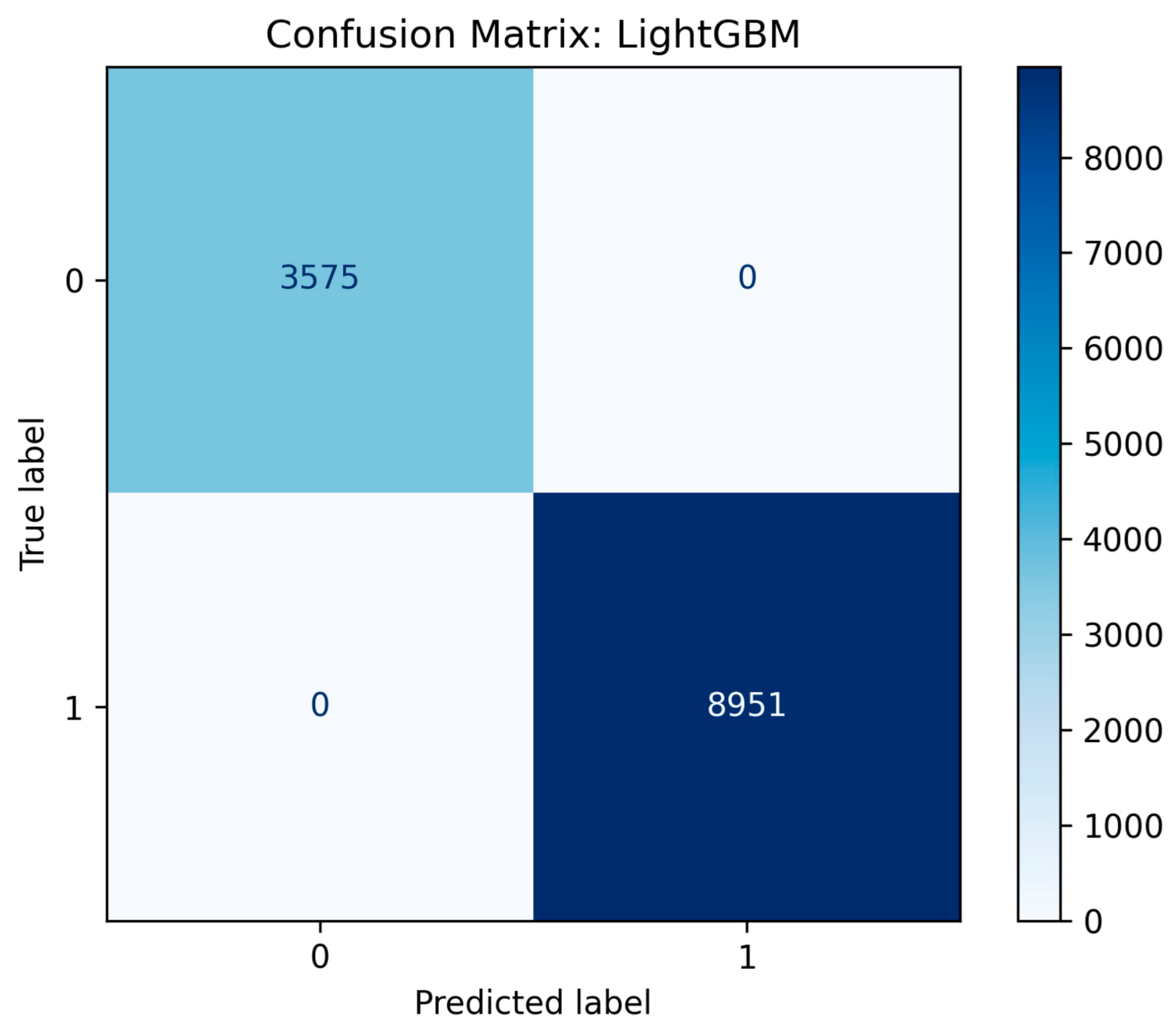
Figure 1.
Confusion matrix results of LightGBM ML model.
4.1.2. Key Findings and Model Selection
Multiple models, including the LightGBM, and DecisionTreeClassifier, achieved perfect F1-Scores (1.0000) and decent real-time processing training times. These results shifted the final selection criteria to model robustness and deployment overhead. On the other hand, it is clearly illustrated that complex models like an NN or SVC, require more training time (63.78 sec and 150.556 sec, respectively), because of their architectures, computation load and data hungry features, making them not suitable for real-time processes in constrained environments and limited amount of data.
The LightGBM model was ultimately selected as the optimal model for the final Psensor component within the hybrid system. While the single Decision Tree model achieved a perfect score of 1.0000 across all metrics (Accuracy, F1-score, and AUC), it presented a critical risk of overfitting, memorizing the specifics of the training data and leading to potential instability when deployed with noisy, real-world sensor readings. The LightGBM model provided virtually identical, perfect performance (e.g., 1.0000 F1-score and 1.0000 AUC), but with superior robustness and regularization, providing more reliable results. This architectural choice ensures significantly better generalization capabilities to new unseen data as well.
4.2. Explainable AI Analysis of RandomForestClassifier (SHAP)
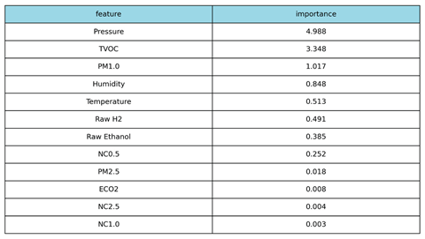
A post-hoc SHAP analysis was performed on the selected LightGBM model to ensure transparency and validate the physical relevance of its decision-making process. The results, reflecting the mean absolute contribution of each feature to the model’s output probability, are presented in Table 2.
4.2.1. Feature Importance Ranking
The SHAP analysis produced the following definitive feature importance ranking for the LightGBM model:
Figure 2.
Bars showcasing features’ importance contribution on model’s final decision-making process.
Figure 2.
Bars showcasing features’ importance contribution on model’s final decision-making process.
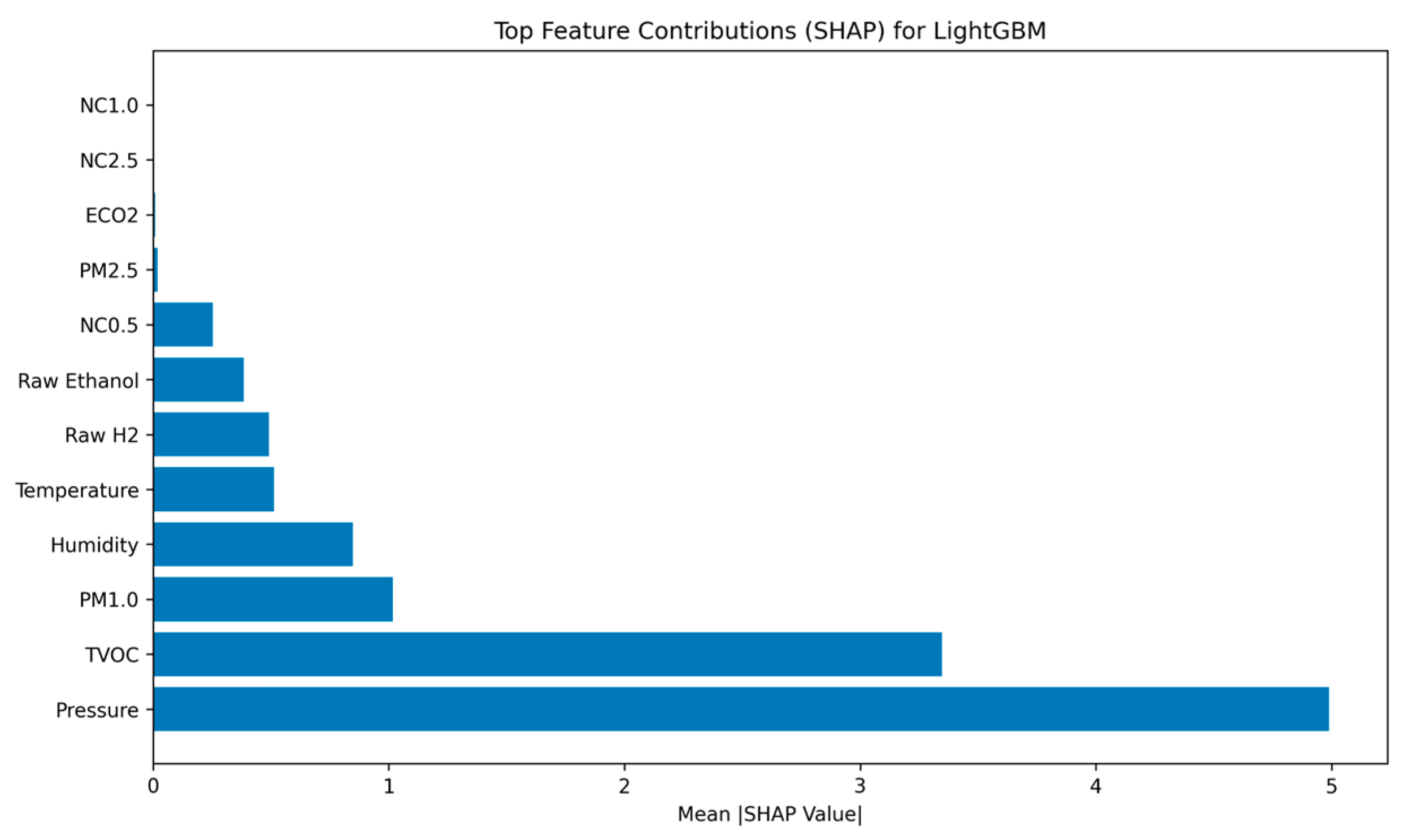
4.2.2. XAI Interpretation
The SHAP ranking confirms that the model’s decision-making is logically sound and aligned with the physical phenomenology of a fire event. Pressure and TVOC (Total Volatile Organic Compounds) are the dominant features, confirming that the model effectively integrates specialized chemical signatures and associated atmospheric changes. The simultaneous high ranking of these two distinct sensor types contributes significantly to the system’s low false-positive rate. Metrics commonly associated with environmental noise, such as Temperature (Rank 5) and eCO2 (Rank 10), are correctly de-prioritized, demonstrating that the classifier relies on complex chemical and pressure patterns rather than simple thermal triggers.
4.3. Comparative Analysis of Vision-Based Detection Nano Models (YOLO Benchmark)
This section details the comparative performance of the five selected YOLO nano variants (v5n, v8n, v10n, v11n, v12n) on the custom Fire and Smoke Image-Label Dataset. The evaluation focuses on the critical trade-off between localization accuracy (mAP) and real-time efficiency (Inference Speed) for edge deployment.
4.3.1. YOLOv5nu Analysis
The YOLOv5nu nano variant establishes a critical baseline, providing a strong balance between localization accuracy and its resource profile. The model achieved a competitive mAP@0.50 of 0.8267 and a satisfactory mAP@0.50-0.95 of 0.5422. These values confirm its high reliability in identifying and accurately bounding both fire and smoke objects across moderate Intersection over Union (IoU > 0.5) and stricter (IoU > 0.95) thresholds.
For real-time industrial deployment, YOLOv5nu provides an Inference Speed of 8.5 to 10.5 FPS (frames per second). While this speed exceeds the minimum required throughput for near real-time monitoring, it leaves limited overhead for more demanding hardware or higher video resolutions. With a compact architecture of 2.6 million parameters, YOLOv5nu is lightweight, but the newer, more optimized architectures have superior speed-to-accuracy trade-offs.
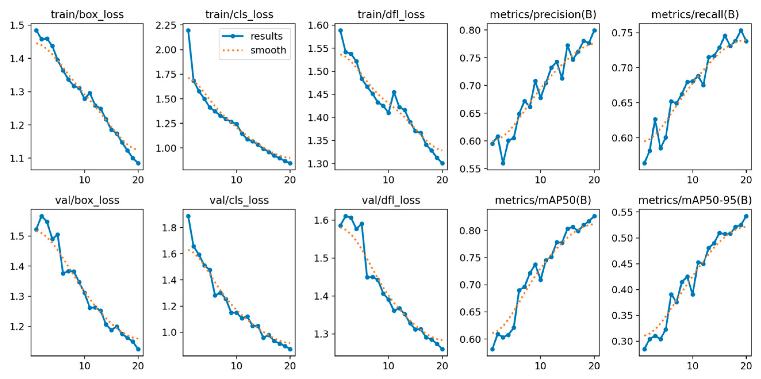
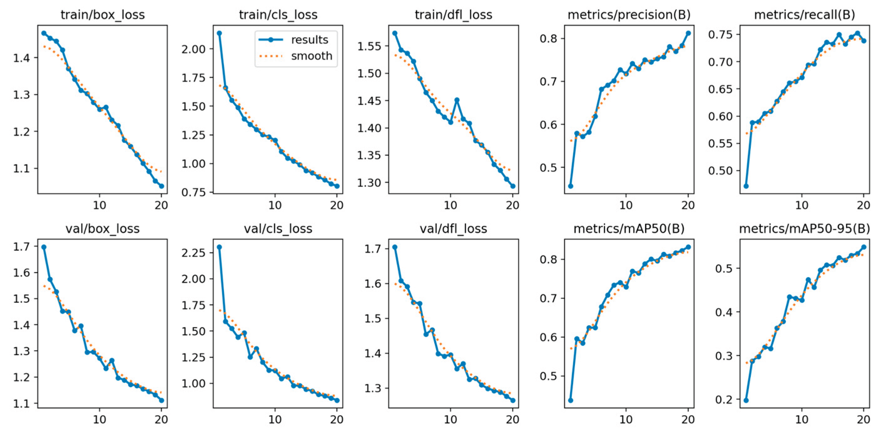
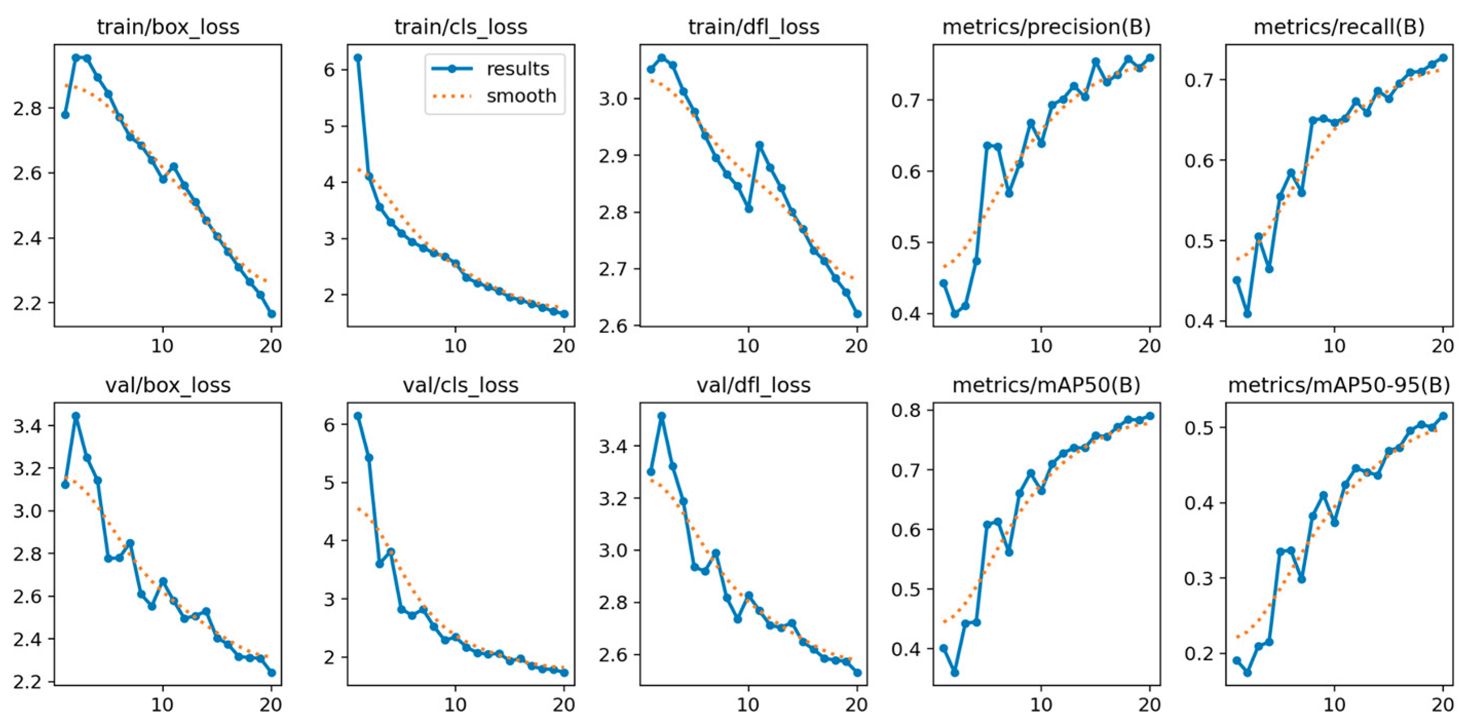
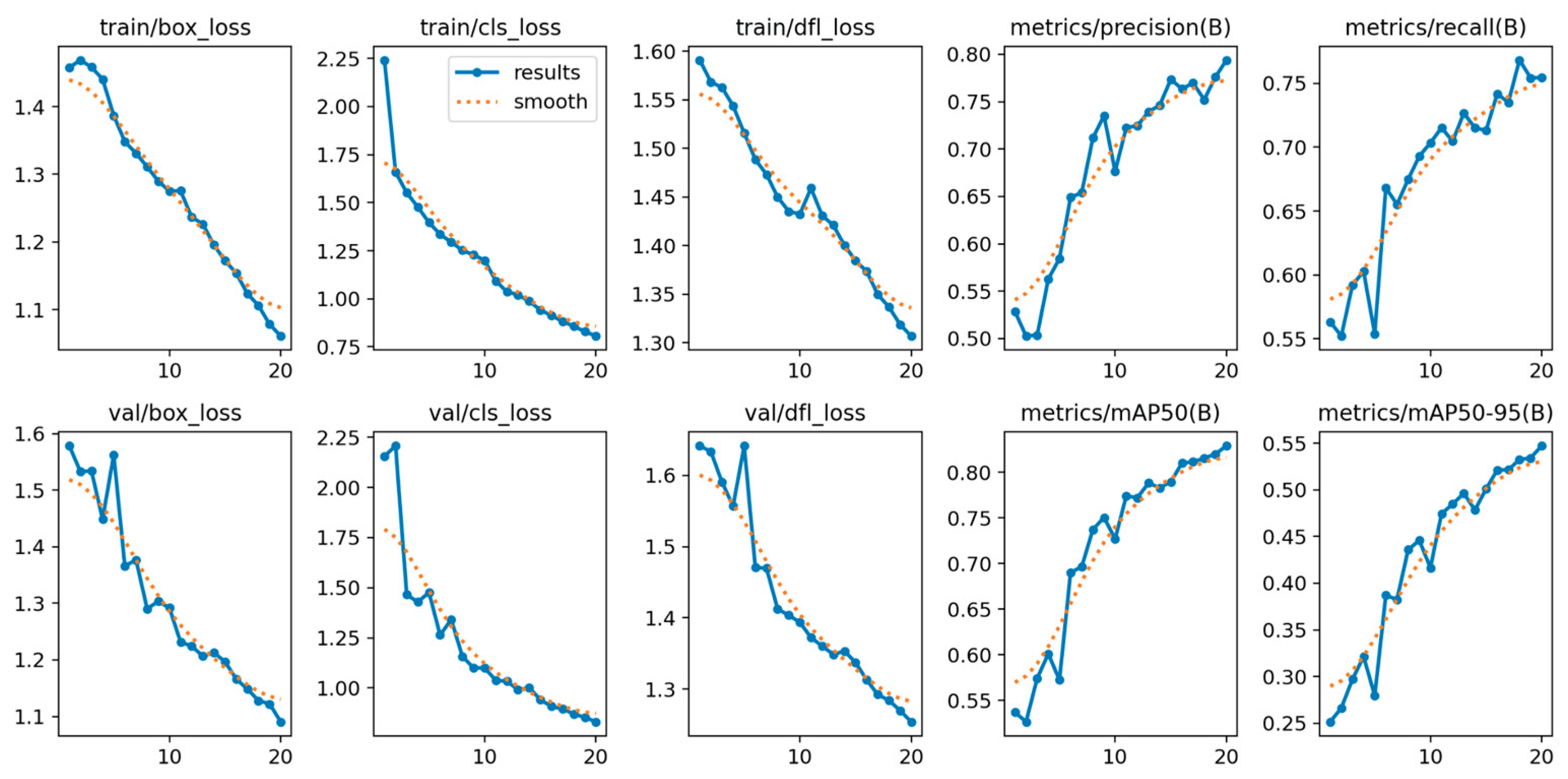
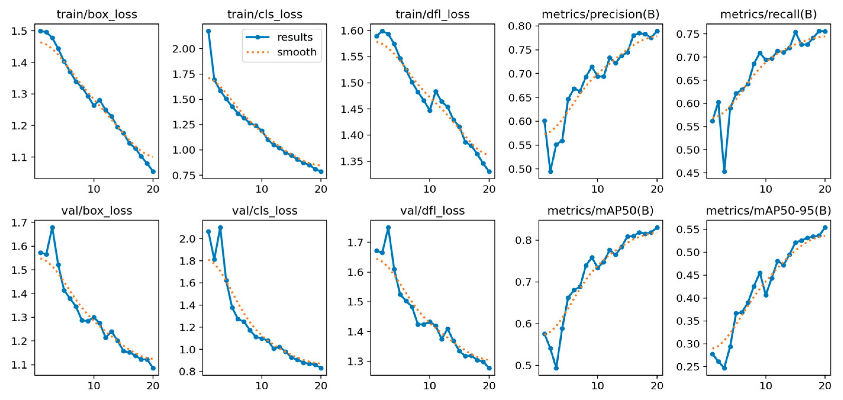
In addition, performance analysis of the training metrics (including train/box_loss, val/cls_loss, and epoch-based precision/recall) confirmed the model’s stable and rapid convergence. The consistent decrease in loss across both training and validation sets, coupled with the monotonic increase in epoch-based precision and recall, indicates that the model did not suffer from significant overfitting or underfitting. This stability validates the model’s robustness and the effectiveness of the chosen training configuration.
Figure 3.
Normalized confusion matrix of smoke/fire detection using YOLOv5nu.

Figure 4.
F1-Confidence metric performance results of YOLOv5nu.
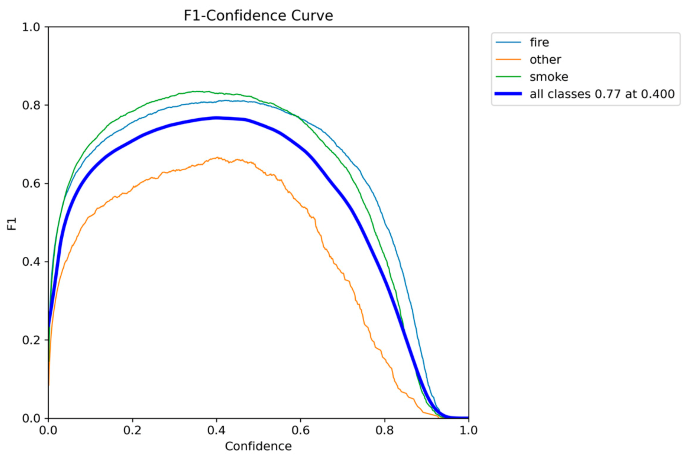
Figure 5.
Precision-Confidence performance results of YOLOv5nu.
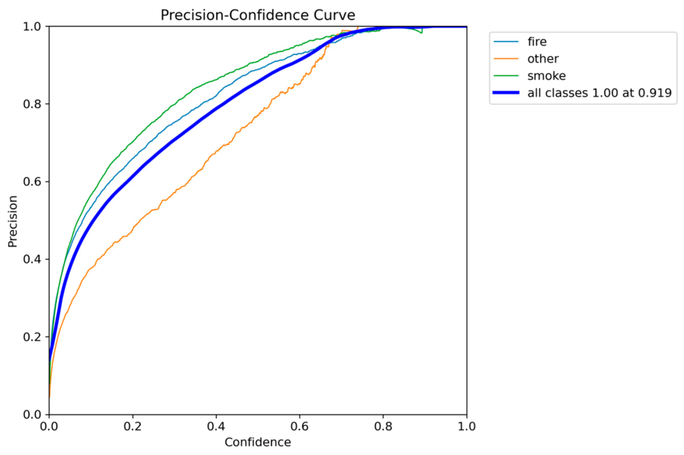
Figure 6.
Precision-Recall performance results of YOLOv5nu.
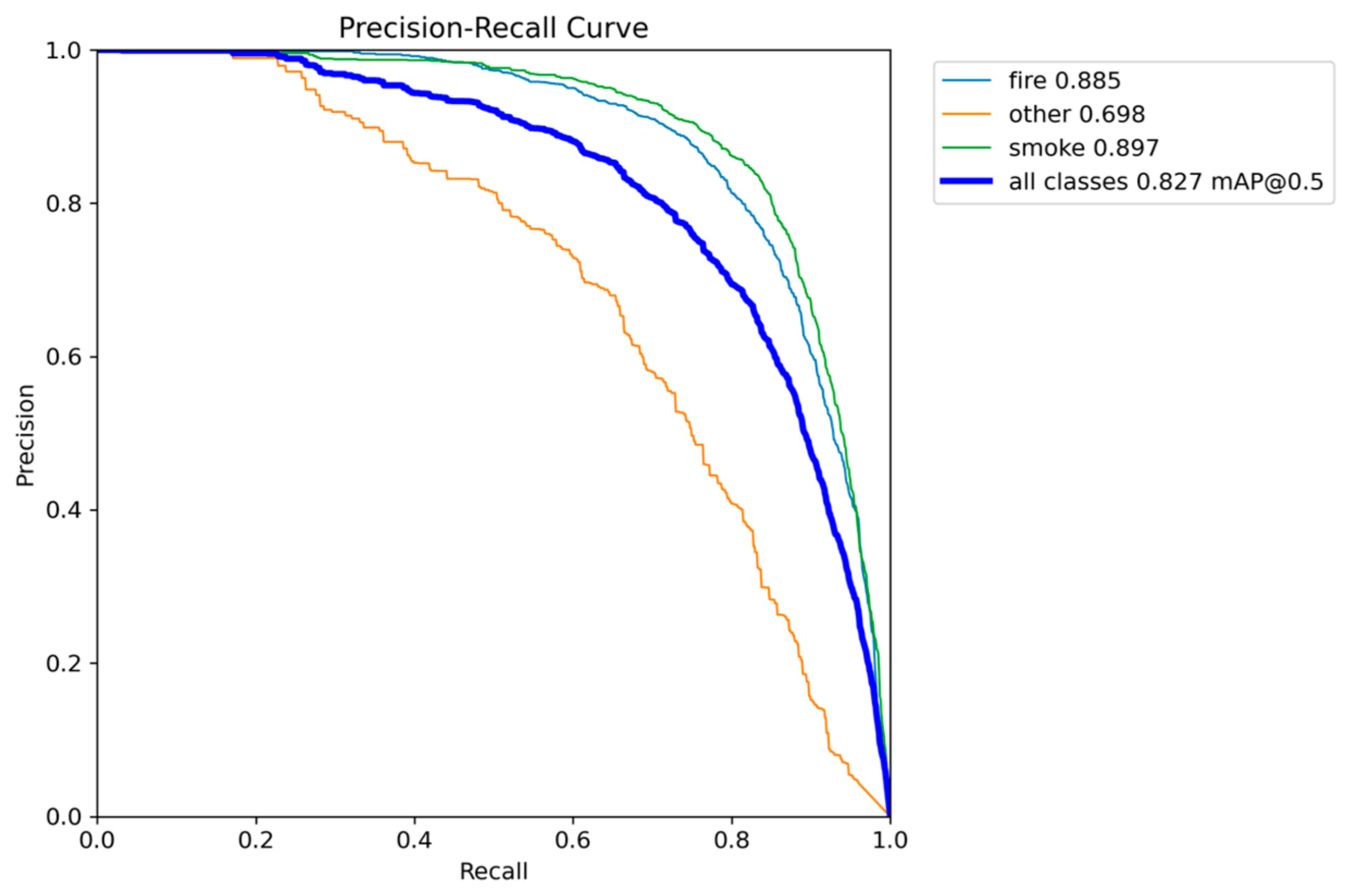
Figure 7.
Recall-Confidence performance results of YOLO5nu.
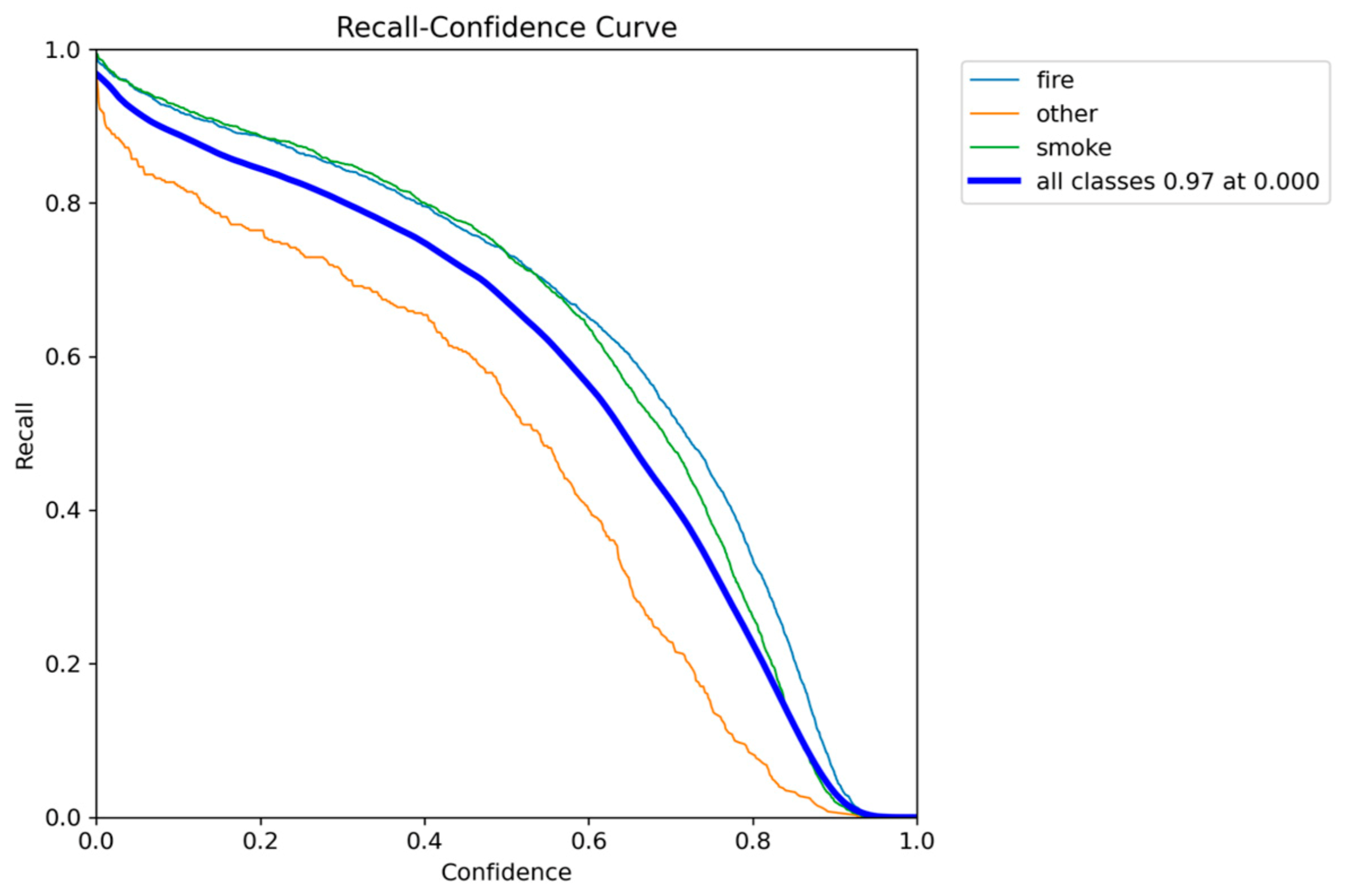
Figure 8.
Different metrics performance results of YOLOv5nu.
Below, Figure 9, illustrates the detections of the YOLOv5nu model, which can detect from small to larger smoke and fire regions successfully.
4.3.2. YOLOv8n Analysis
The YOLOv8n model presents additional gains in accuracy while maintaining a constrained resource footprint. It achieved the best overall performance, obtaining the highest mAP@0.50 of 0.8320 and a marginal increase and second best in comprehensive localization accuracy, with mAP@0.50-0.95 reaching 0.5489. This indicates a minor increase in the model’s ability to precisely localize fire and smoke objects, particularly at stricter IoU thresholds.
However, in terms of efficiency, YOLOv8n exhibited a slight performance degradation compared to YOLOv5n, achieving an Inference Speed of 7.5 to 9.5 FPS. While this speed still meets the minimum real-time requirement for the edge device, it is slower than the v5nu baseline, but still the second best one, among the YOLO nano models. The model’s complexity increased to 3.2 million parameters, making it slightly larger. This suggests that the architectural improvements place YOLOv8n among nano-scale YOLO variants, as the most favorable trade-off, between detection accuracy and inference speed, making it the most suitable model for real-time smoke and fire detection on resource-constrained edge devices.
Finally, the analysis of the YOLOv8n training metrics (such as the bounding box loss, which finalized at approximately 1.1117) confirmed highly stable and robust learning. The smooth, consistent decrease in loss across both the training and validation sets indicates that the model converged effectively without significant oscillation or divergence.
Figure 10.
Normalized confusion matrix of smoke/fire detection using YOLOv8n.
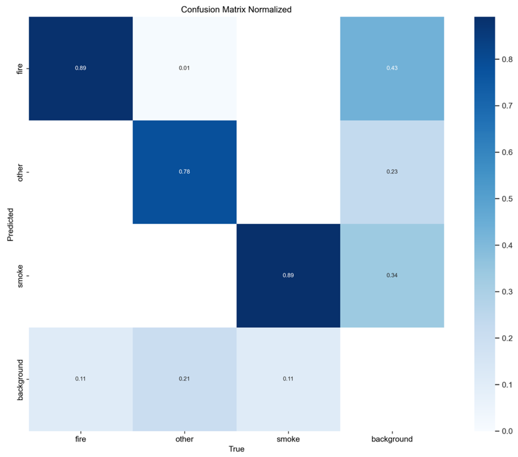
Figure 11.
F1-Confidence performance results of YOLOv8n.
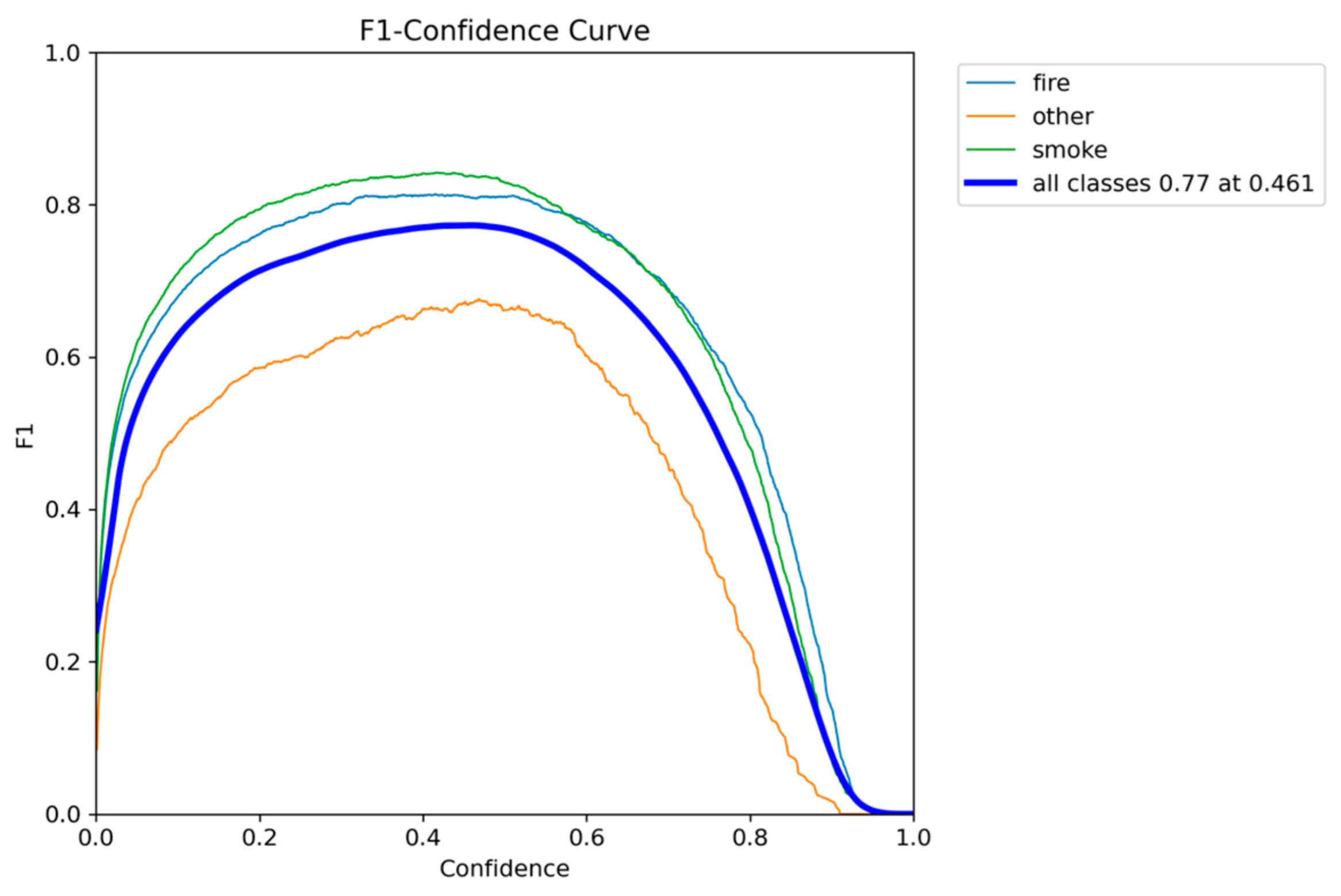
Figure 12.
Precision-Confidence performance results of YOLOv8n.

Figure 13.
Precision-Recall performance results of YOLOv8n.

Figure 14.
Recall-Confidence performance results of YOLOv8n.
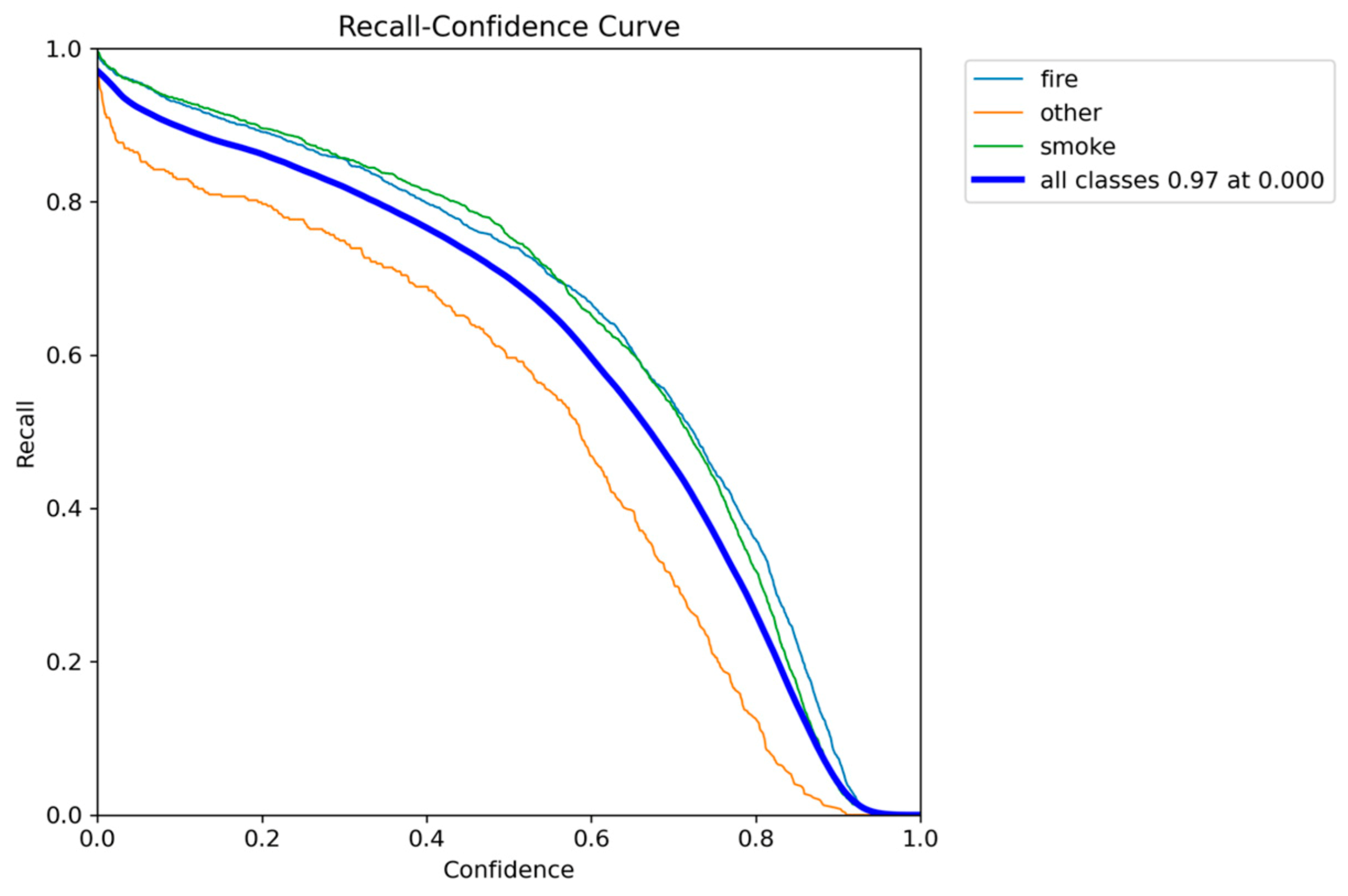
Figure 15.
Different metrics performance results of YOLOv8n.
Below, Figure 16, illustrates the detections of the YOLOv8n model, which can detect from small to larger smoke and fire regions successfully.
4.3.3. YOLOv10n Analysis
The YOLOv10n model presents a noticeable shift in the accuracy-speed trade-off compared to its predecessors. It is the most lightweight model so far, with a size of 2.3 million parameters, making it highly attractive for the most resource-constrained devices. It also maintains competitive inference speed, ranging from 6.9 to 9.5 FPS. This speed means that while it is highly compact, its real-time performance is variable and can drop below the desired 7 FPS threshold, posing a reliability risk.
In terms of accuracy, YOLOv10n achieved a mAP@0.50 of 0.7906 and a mAP@0.50-0.95 of 0.5156. While these scores are robust, they represent a decline in performance compared to both YOLOv5n and YOLOv8n. This decline suggests that the architectural changes focused on reducing the parameter count finally have an impact on the model’s ability to maximize detection accuracy on the fire and smoke dataset.
The training metrics confirm that the YOLOv10n model successfully converged, indicated by the low difference between the final training box loss (approximately 2.17) and the validation box loss (approximately 2.24). This minimal loss gap suggests that despite the architectural modifications for size reduction, the model trained stably without significant signs of overfitting, confirming the reliability of the reported accuracy figures.
Figure 17.
Normalized confusion matrix of smoke/fire detection using YOLOv10n.
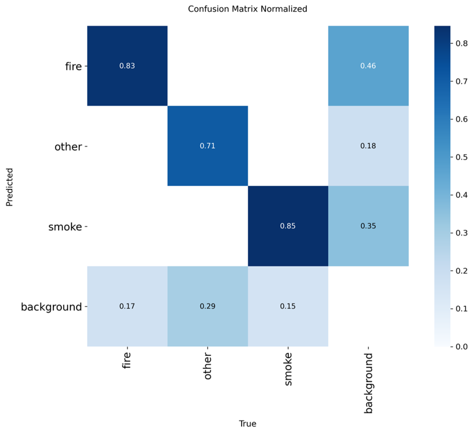
Figure 18.
F1-Confidence performance results of YOLOv10n.
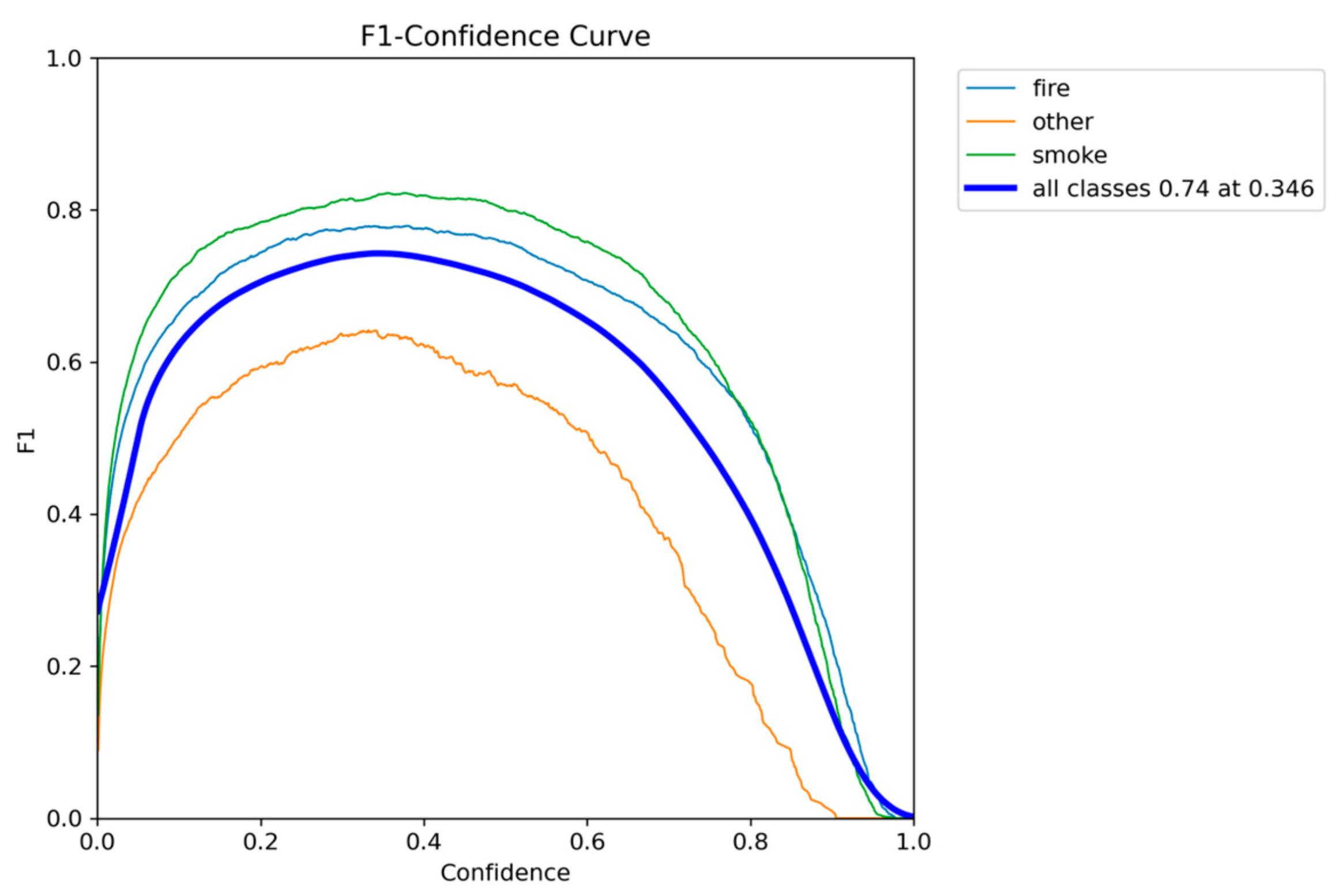
Figure 19.
Precision-Confidence performance results of YOLOv10n.

Figure 20.
Recall-Confidence performance results of YOLOv10n.
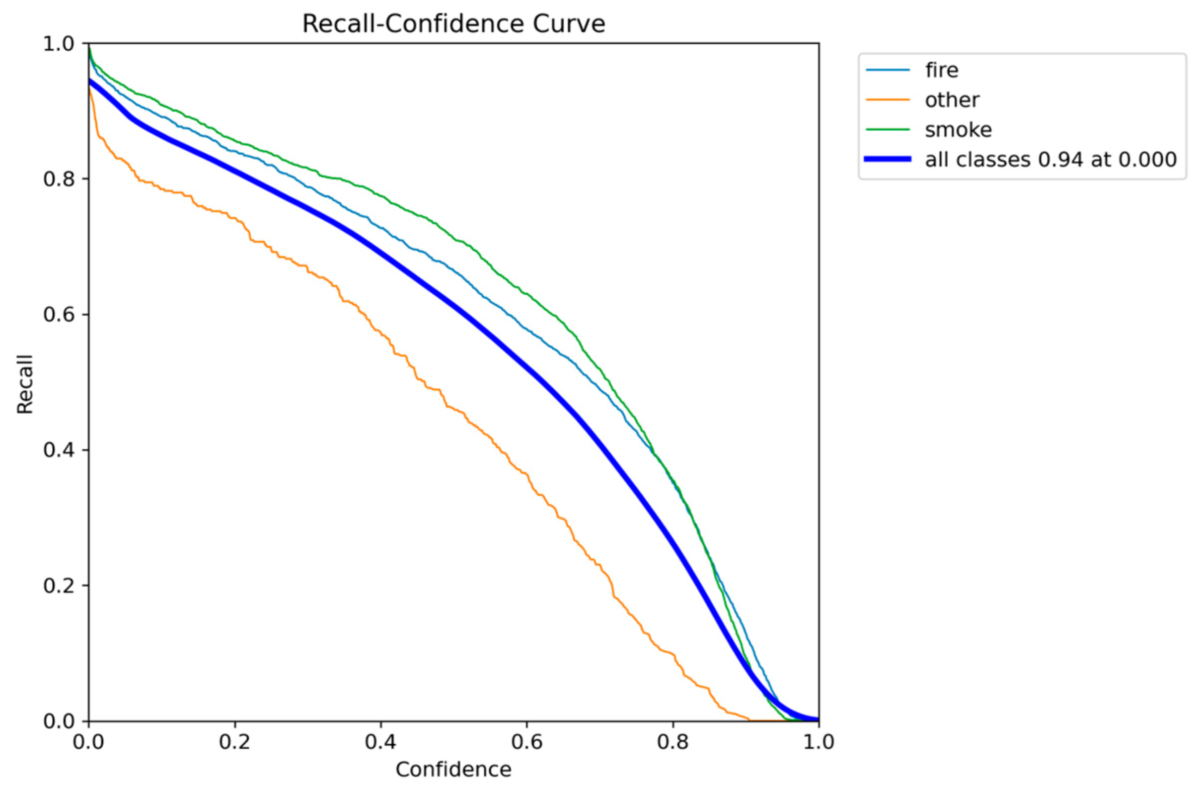
Figure 21.
Precision-Recall performance results of YOLOv10n.
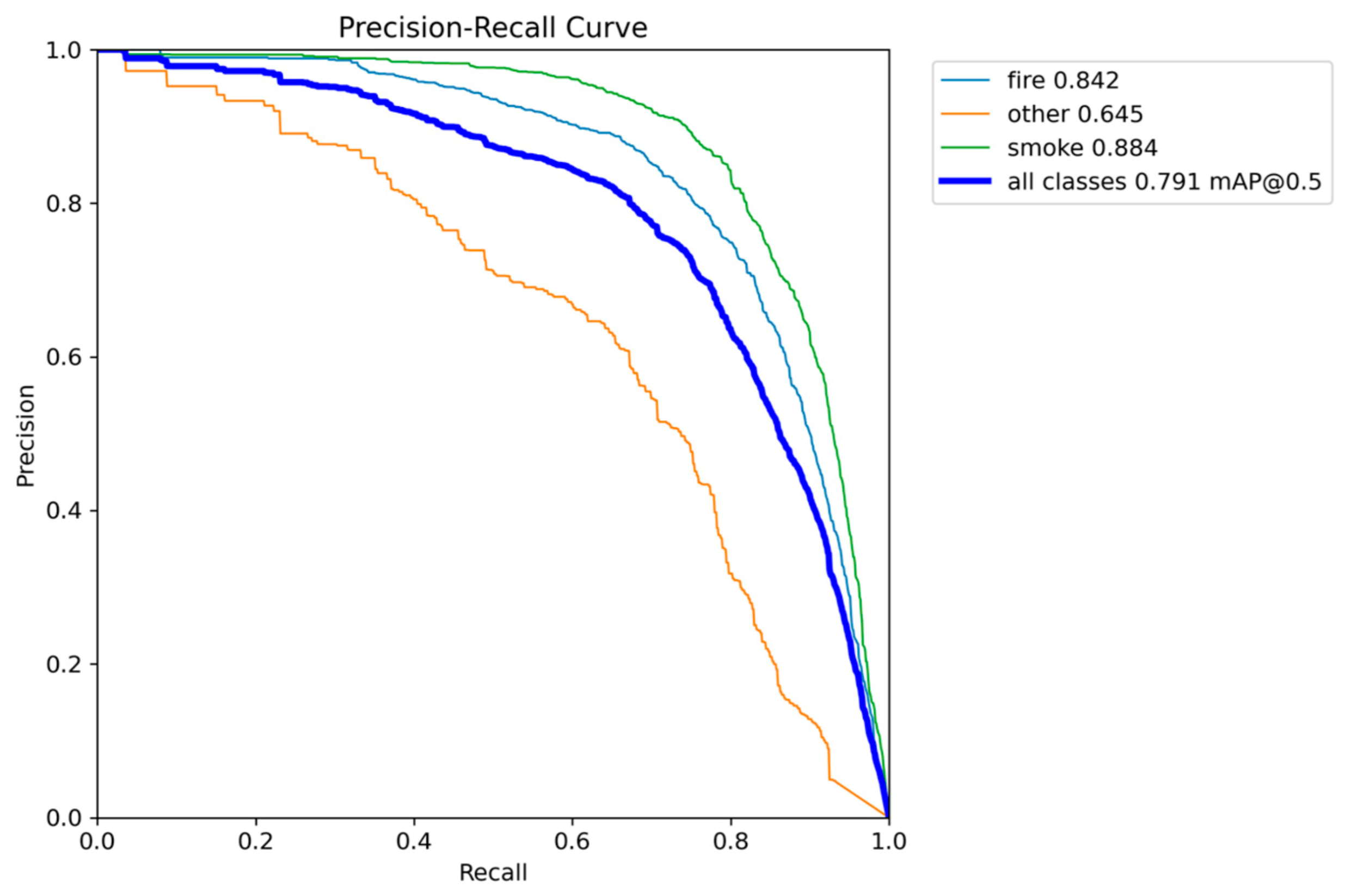
Figure 22.
Different metrics performance results of YOLOv10n.
Below, Figure 23, illustrates the detections of the YOLOv10n model, which can detect from small to larger smoke and fire regions successfully.
4.3.4. YOLOv11n Analysis
The YOLOv11n model achieved a mAP@0.50 of 0.8293 and an mAP@0.50-0.95 of 0.5474. These scores are nearly identical to the high accuracy achieved by the YOLOv8n model, significantly outperforming the low-accuracy YOLOv10n variant. In terms of efficiency, YOLOv11n achieved a favorable parameter count of 2.6 million, which matches the compact size of YOLOv5n and is smaller than YOLOv8n. Its inference speed of 7.0 to 8.9 FPS is stable and consistently meets the real-time threshold (7 FPS), avoiding the risk of performance drops observed in YOLOv10n.
The final analysis of the YOLOv11n training data confirms excellent convergence stability. The final training box loss (approximately 1.06) and validation box loss (approximately 1.09) are both very low and tightly coupled.
Figure 24.
Normalized confusion matrix of smoke/fire detection using YOLOv11n.
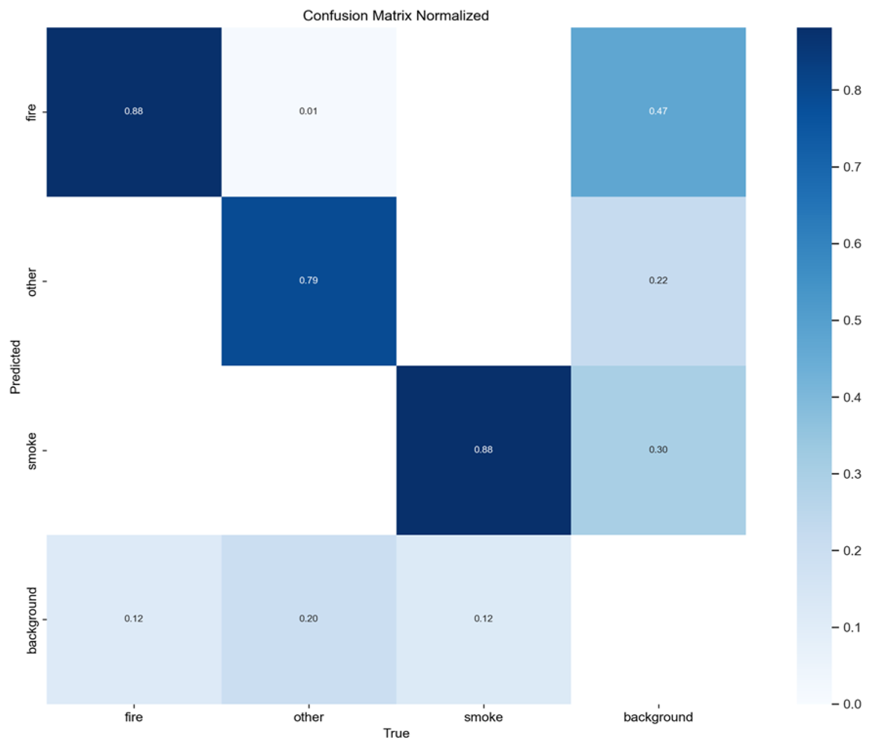
Figure 25.
F1-Confidence performance results of YOLOv11n.

Figure 26.
Precision-Confidence performance results of YOLOv11n.

Figure 27.
Recall-Confidence performance results of YOLOv11n.
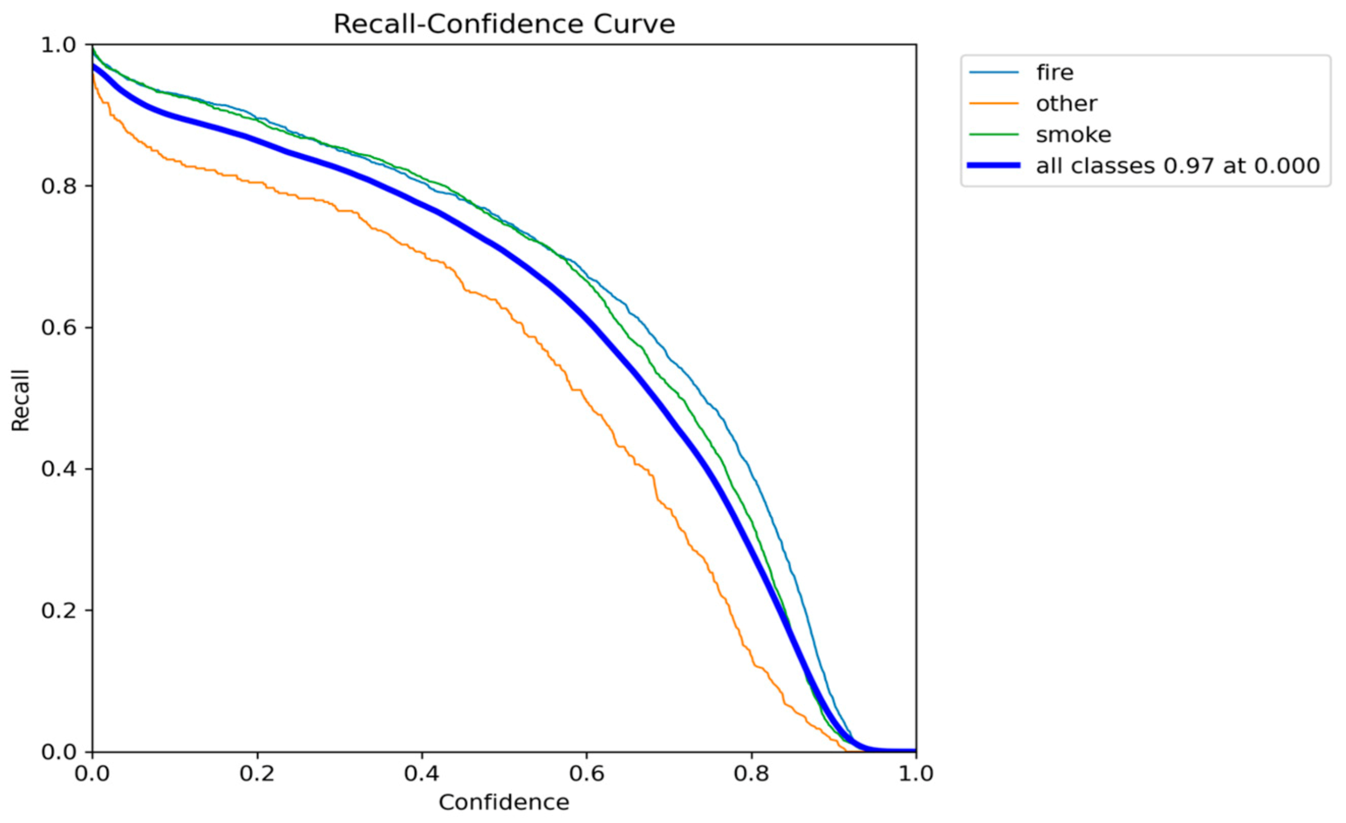
Figure 28.
Precision-Recall performance results of YOLOv11n.
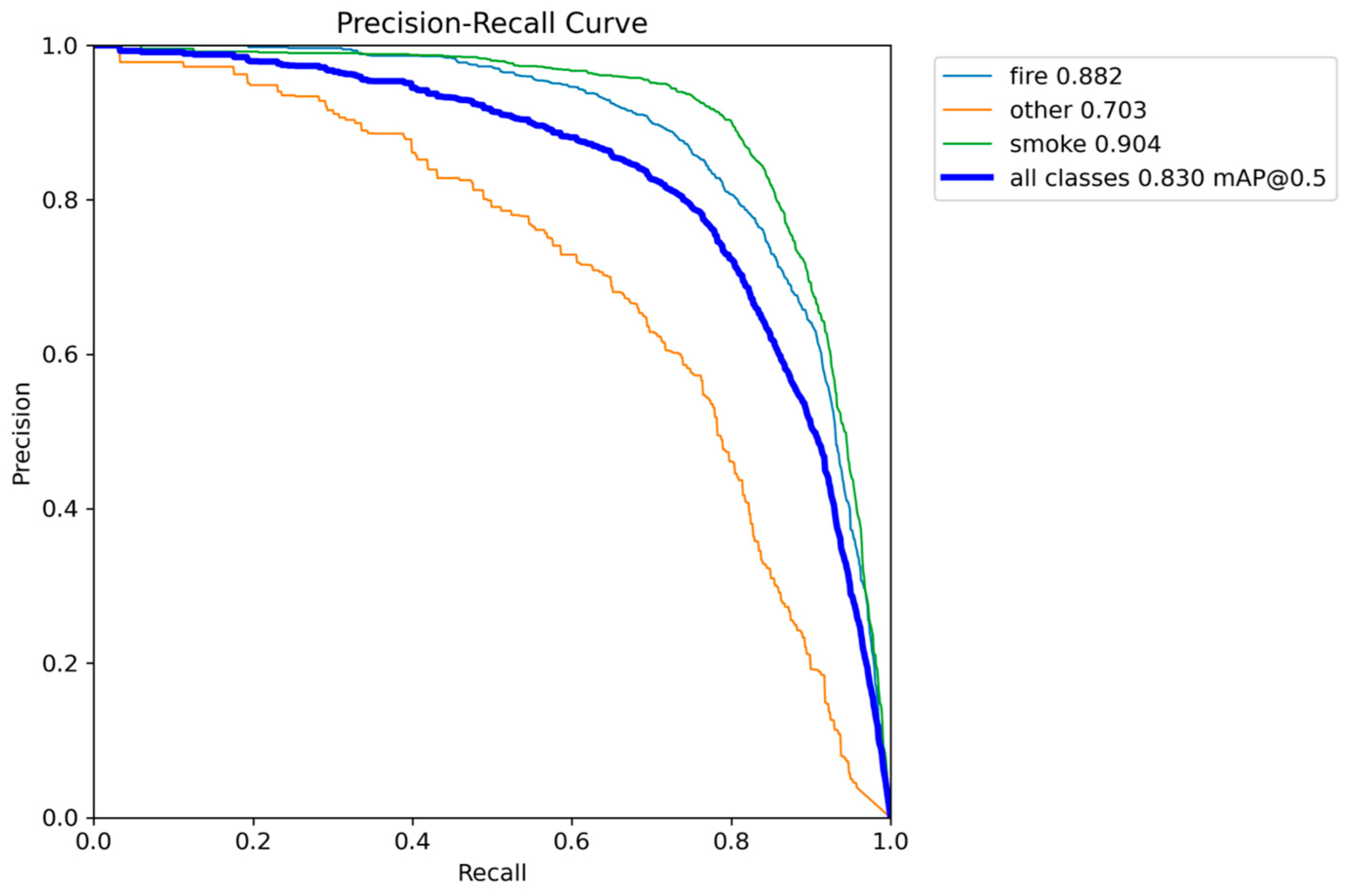
Figure 29.
Different metrics performance results of YOLOv11n.
Below, Figure 30, illustrates the detections of the YOLOv11n model, which can detect from small to larger smoke and fire regions successfully.
4.3.5. YOLOv12n Analysis
The YOLOv12n model demonstrates the highest overall localization accuracy among all nano variants benchmarked, achieving a mAP@0.50-0.95 score of 0.5544 and the second best mAP@0.50 of 0.8306. This high mAP@0.50-0.95 value indicates its superior ability to place highly precise bounding boxes around fire and smoke, even at very strict IoU thresholds. The model maintains a compact structure of 2.6 million parameters, matching YOLOv5n and YOLOv11n in size.
However, YOLOv12n showed the slowest Inference Speed of 6.2 to 7.3 FPS. Since the minimum real-time requirement for the target edge device is 7 FPS, this model is almost unreliable for true real-time deployment on our hardware edge device, as its performance frequently drops below the critical threshold.
The training metrics for YOLOv12n confirm exceptional learning optimization. The final training box loss (approximately 1.05) and validation box loss (approximately 1.09) are extremely low and tightly matched, signifying near-perfect convergence and superb generalization capability. This stability validates the model’s accuracy but confirms that its performance limitation lies strictly in its architectural complexity during inference.
Figure 31.
Normalized confusion matrix of smoke/fire detection using YOLOv12n.
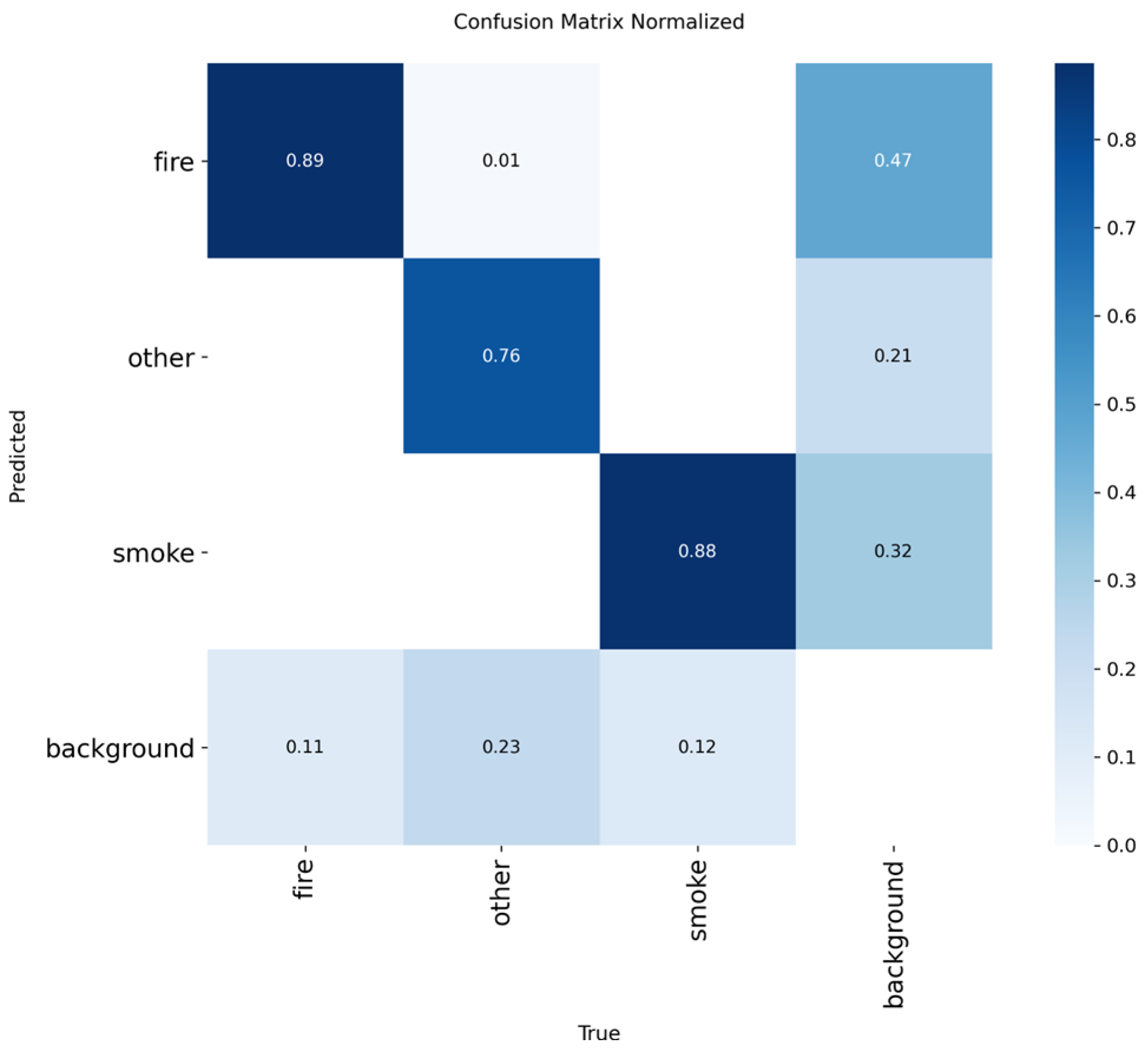
Figure 32.
F1-Confidence performance results of YOLOv12n.
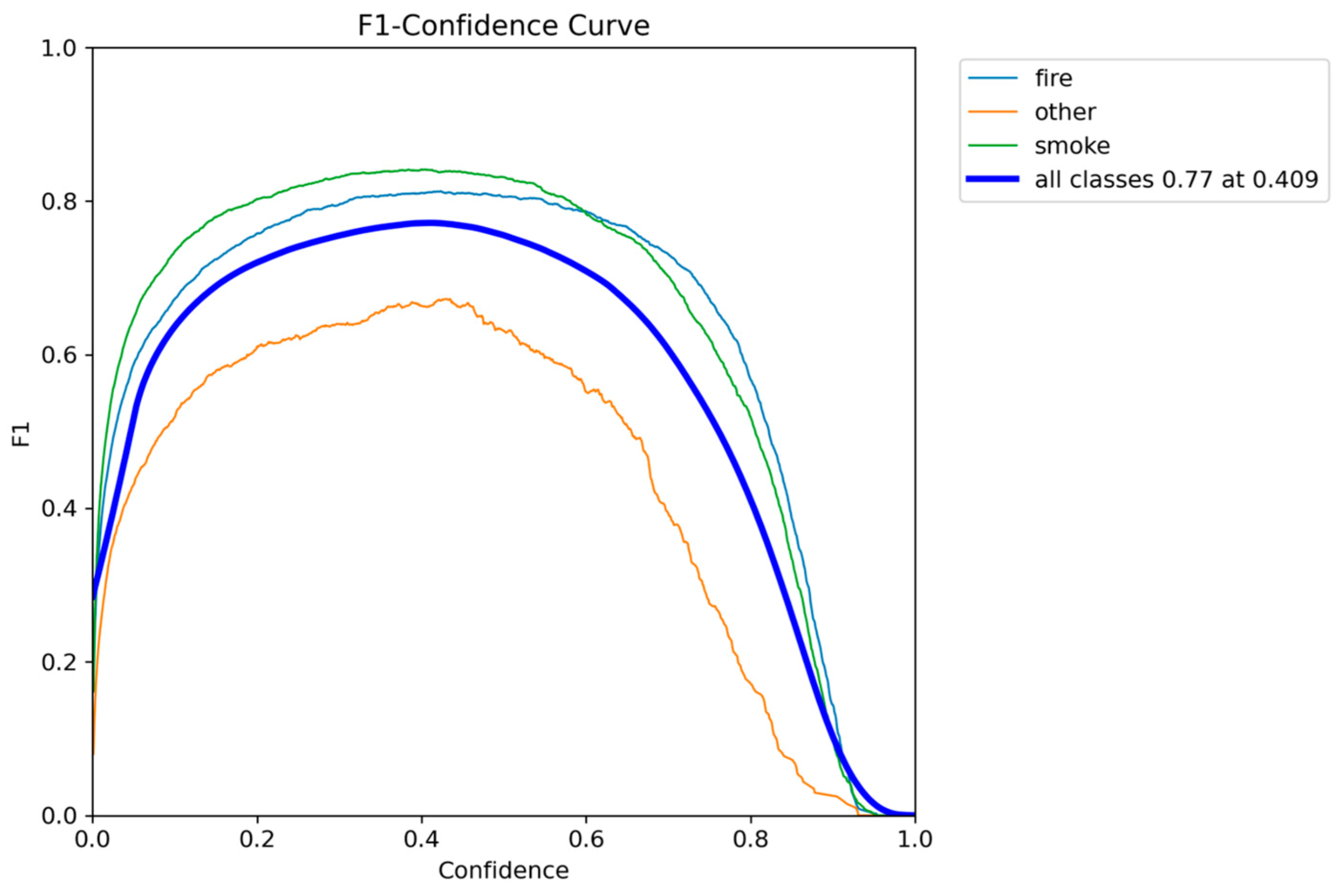
Figure 33.
Precision-Confidence performance results of YOLOv12n.

Figure 34.
Recall-Confidence performance results of YOLOv12n.
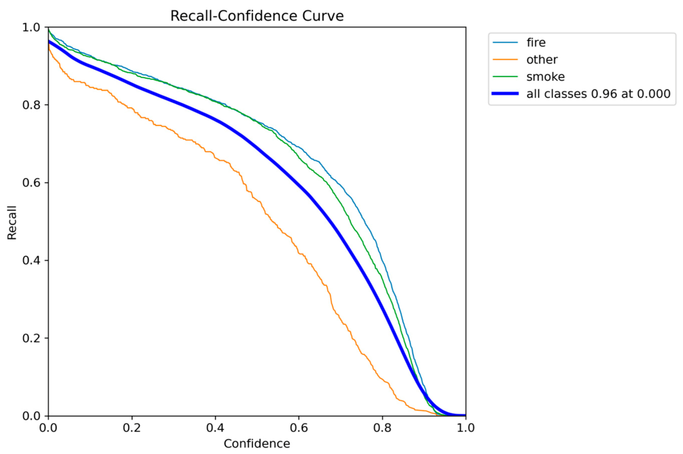
Figure 35.
Precision-Recall performance results of YOLOv12n.

Figure 36.
Different metrics performance results of YOLOv12n.
Below, Figure 37, illustrates the detections of the YOLOv12n model, which can detect from small to larger smoke and fire regions successfully.
4.3.6. Comparative Analysis and Optimal Model Selection
The comparative analysis of the five YOLO nano models reveals a clear trade-off spectrum between accuracy, model size, and real-time inference speed, which is summarized below:

Table 3.
Presenting the final mAP@0.50, mAP@0.50-0.95 and FPS performance results for each YOLO nano model.
Table 3.
Presenting the final mAP@0.50, mAP@0.50-0.95 and FPS performance results for each YOLO nano model.
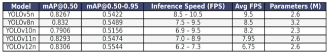 |
Figure 38.
Presenting the final mAP@0.50, mAP@0.50-0.95 and FPS performance results for each YOLO nano model.
Figure 38.
Presenting the final mAP@0.50, mAP@0.50-0.95 and FPS performance results for each YOLO nano model.
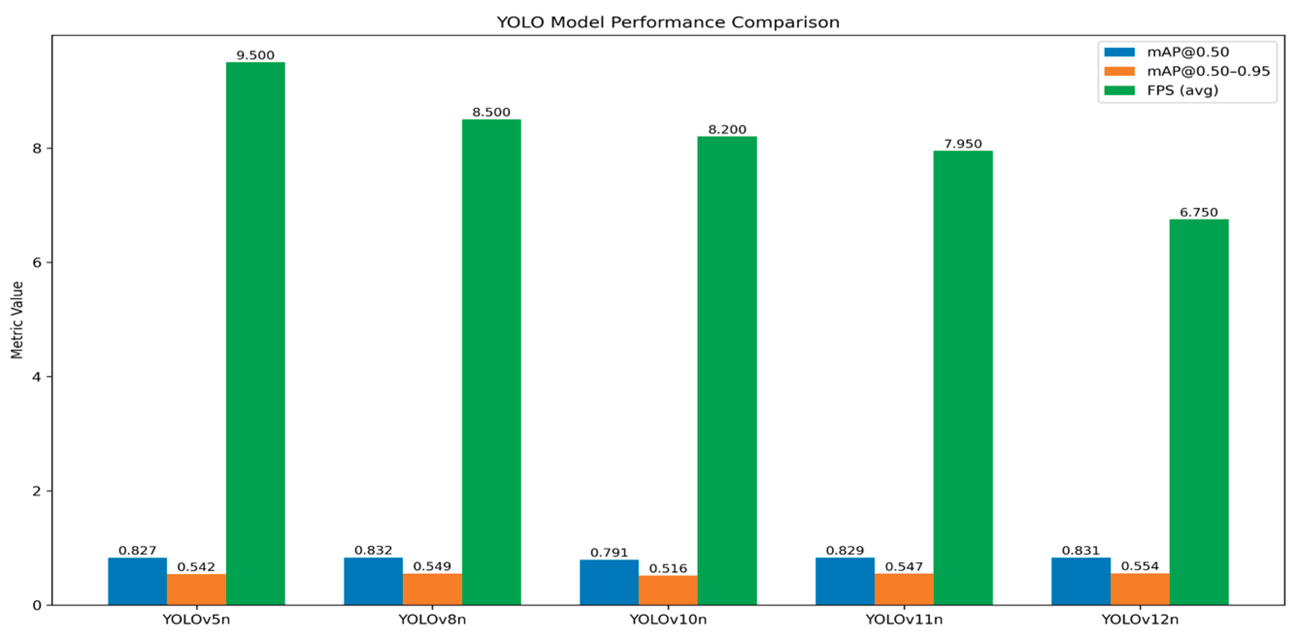
Models like YOLOv12n achieved the highest overall localization accuracy with an mAP@0.50-0.95 of 0.5544, but its slow inference speed (6.2 to 7.3 FPS) makes it unreliable for the target 7 FPS real-time deployment threshold. Conversely, YOLOv10n was the most compact (2.3 million parameters) but compromised too much on accuracy, achieving the lowest mAP@0.50 of 0.7906. YOLOv11n provided a strong balance with high accuracy (0.8293 mAP@0.50) and a compact 2.6 million parameters, but its speed (minimum 7.0 FPS) was too close to the critical limit. Although YOLOv5nu achieved marginally higher inference speed [8.5–10.5 FPS] and decent mAP@0.50 of 0.8267 and mAP@0.50-0.95 of 0.5422, given the necessity for robust, high-speed performance on a lightweight edge device, YOLOv8n was selected as the optimal model, providing the best and excellent detection accuracy (0.8320 mAP@0.50) and the second-best mAP@0.50-0.95 of 0.5489 with a compact size (3.2 million parameters), as well as a decent and stable inference speed (ranging from 7.5 to 9.5 FPS).
4.4. Explainable AI (XAI) Analysis of Detection Models
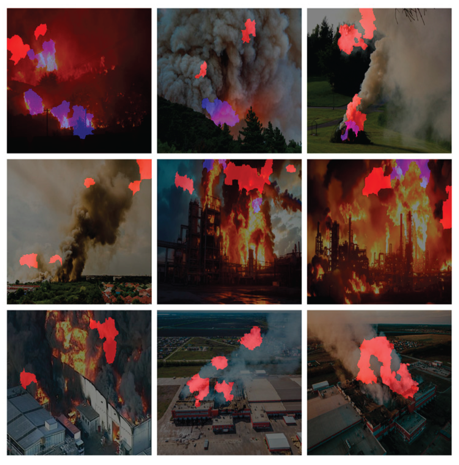
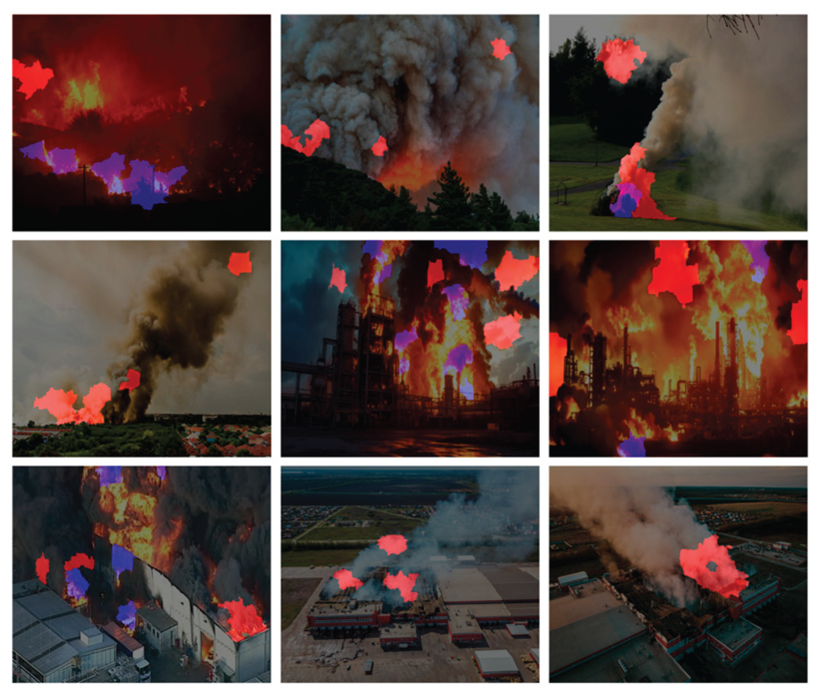
In order to provide insight into the detection mechanism of the chosen models and validate their decision-making process, LIME was employed as the post-hoc eXplainable AI technique, applied on images. This analysis was systematically performed on each YOLO nano variant (YOLOv5n, v8n, v10n, v11n, and v12n), utilizing the exact same set of nine test images [44,45,46,47,48,49,50,51,52] for every model to ensure a fair, direct comparison of interpretability. LIME works by approximating the complex model’s prediction locally, visually isolating the specific input features (pixels) that most contributed to the model’s output. The resulting heatmaps highlight the most contributing area for detection with a distinct color coding applied: areas contributing to the ‘fire’ class (Class 0) were highlighted in blue, and areas contributing to the ‘smoke’ class (Class 2) were highlighted in red.
4.4.1. YOLOv5nu
The analysis of the YOLOv5n LIME superplot reveals a highly focused and efficient feature selection strategy across the nine test images. The LIME heatmaps, which highlight features contributing to the ‘fire’ class in blue and the ‘smoke’ class in red, demonstrate a tight concentration of contributing pixels precisely over the core regions of the detected objects. The model presents minimal diffusion of feature importance into non-relevant background areas, confirming that its architectural design enables it to make reliable detection decisions based only on the most necessary visual evidence.
Figure 39.
Applying LIME XAI for feature/area contribution importance on nine images using YOLOv5nu.
Figure 39.
Applying LIME XAI for feature/area contribution importance on nine images using YOLOv5nu.
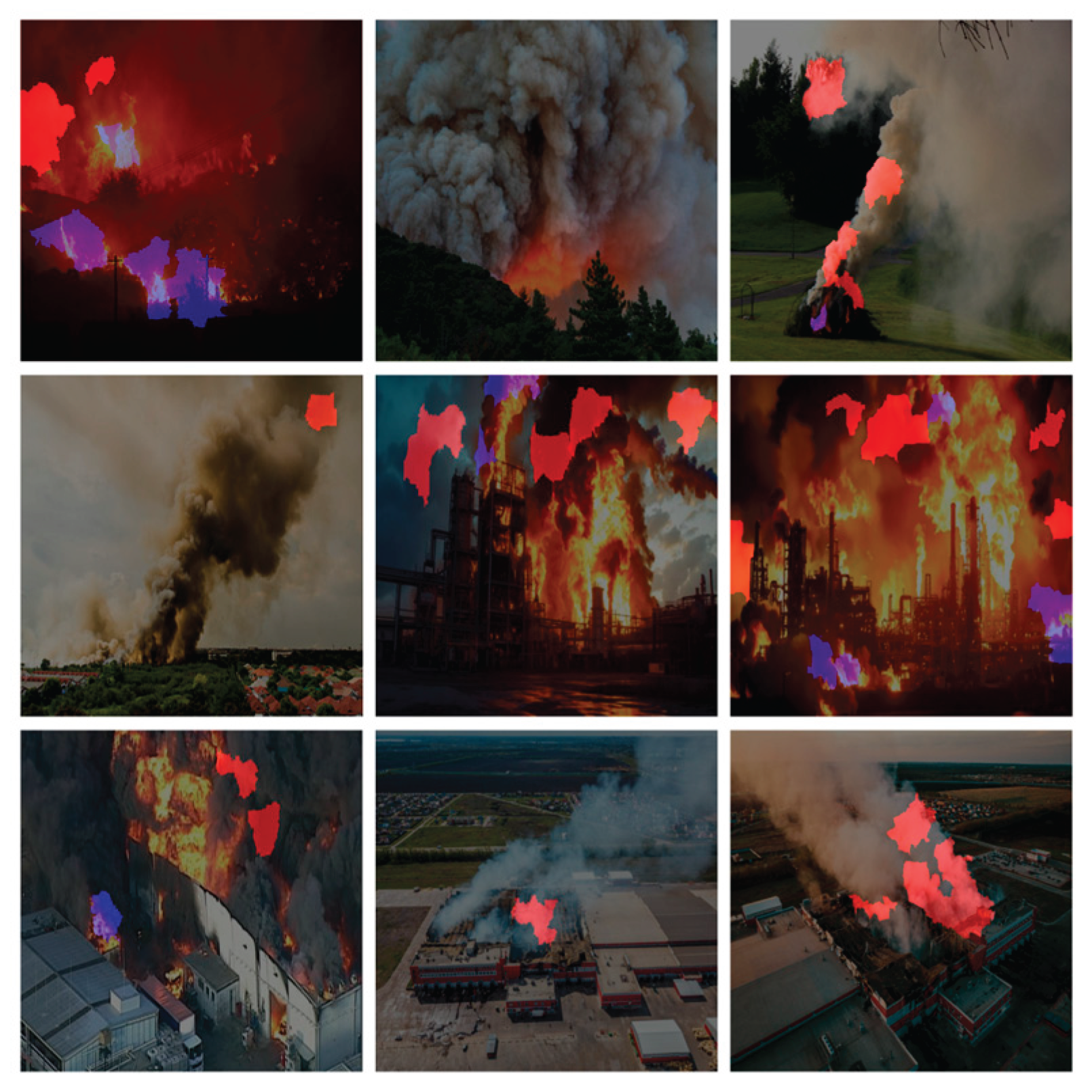
4.4.2. YOLOv8n
In YOLOv8n, while the heatmaps successfully isolate the objects, showing fire in blue and smoke in red concentrated over the correct regions, the explanations are visually denser and slightly more diffused compared to the previous model. YOLOv8n frequently incorporates a wider perimeter of pixels around the fire and smoke plumes and utilizes a slightly more extensive feature set from the immediate background to confirm its highly accurate detections. This reliance on a broader, more context-rich feature map to achieve its high localization quality is visually confirmed by the LIME output.
Figure 40.
Applying LIME XAI for feature/area contribution importance on nine images using YOLOv8n.

4.4.3. YOLOv10n
In YOLOv10n, XAI output presents a significant degree of fragmentation and instability in the model’s feature selection when compared to the other cases. While the contributing features (fire in blue, smoke in red) are broadly positioned over the correct objects, the heatmaps are frequently discontinuous and scattered. In several of the nine test images, the model’s focus is clearly incomplete, failing to incorporate critical features like the base of a flame or the dense center of a smoke cloud. Furthermore, there is an increased tendency for fragmented importance to appear in irrelevant background regions, which is indicative of a less reliable and more confused decision-making process.
Figure 41.
Applying LIME XAI for feature/area contribution importance on nine images using YOLOv10n.
Figure 41.
Applying LIME XAI for feature/area contribution importance on nine images using YOLOv10n.
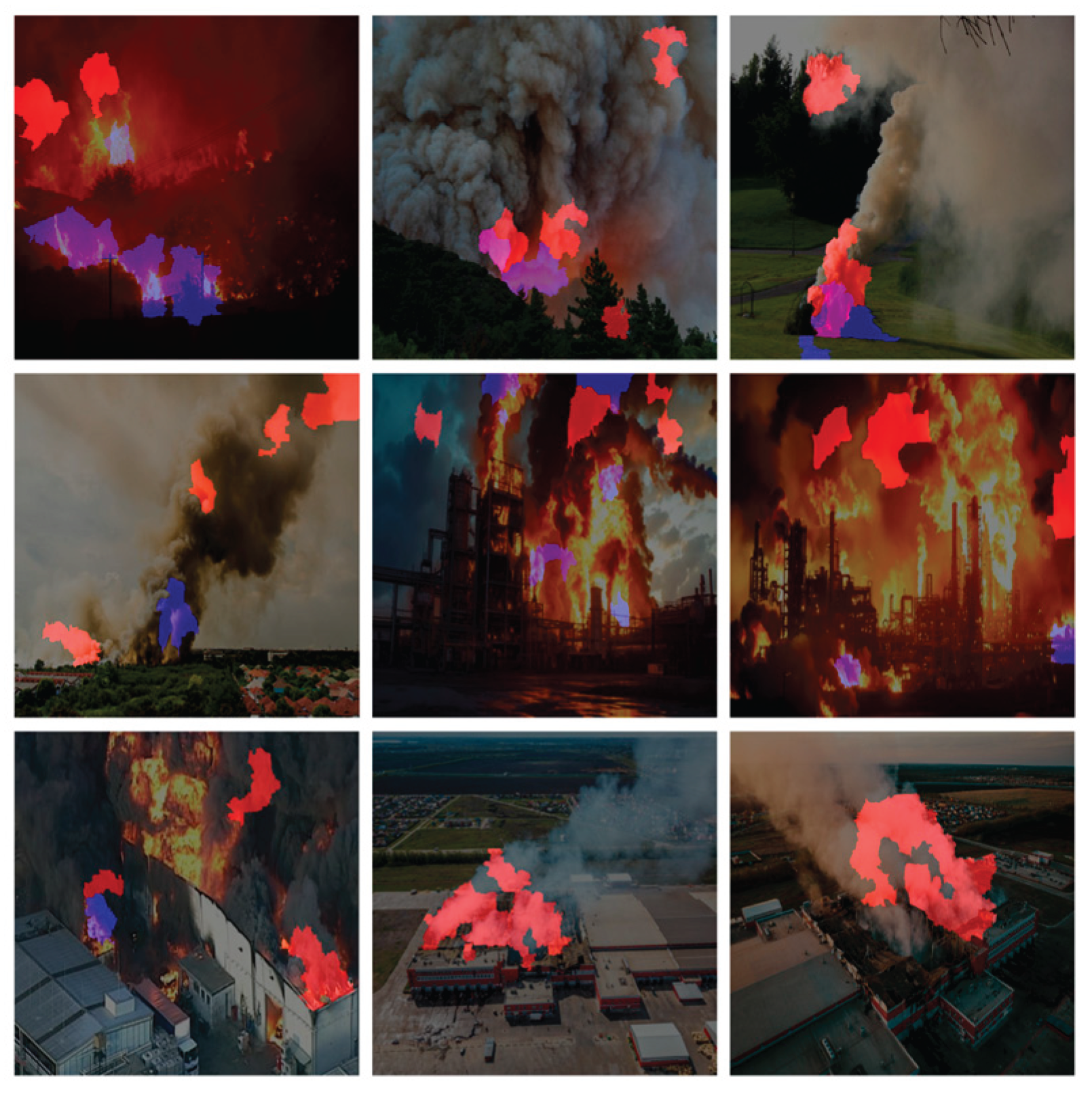
4.4.4. YOLOv11n
In YOLOv11n, a near-optimal balance between focused interpretation and high accuracy is achieved. The heatmaps present and efficient feature selection strategy observed in YOLOv5n, yet the explanations retain the comprehensive object coverage associated with the higher-accuracy variants. Features contributing to ‘fire’ (blue) and ‘smoke’ (red) are sharply localized and highly cohesive, maintaining robust object coverage without the excessive diffusion or background noise seen in YOLOv8n. In the same context, the explanations are highly stable and complete across all nine test images, visually confirming that the model’s compact parameter count (2.6 million) does not compromise its ability to reliably and accurately extract necessary visual information.
Figure 42.
Applying LIME XAI for feature/area contribution importance on nine images using YOLOv11n.
Figure 42.
Applying LIME XAI for feature/area contribution importance on nine images using YOLOv11n.
4.4.5. YOLOv12n
Lastly, the qualitative LIME analysis for YOLOv12n provides a clear visual correlation for its performance extremes—namely, its industry-leading localization accuracy achieved at the expense of speed. Across the nine test images, the heatmaps are visually the most detailed and extensive of all five variants. The features contributing to ‘fire’ (blue) and ‘smoke’ (red) are highly concentrated, and the model has improved performance at incorporating the fringe pixels and boundary regions of the objects. The comprehensive, high-resolution coverage across the object boundaries visually explains the model’s significant computational load and its resultant penalty in inference speed, validating its supreme localization capability at the cost of real-time efficiency.
Figure 43.
Applying LIME XAI for feature/area contribution importance on nine images using YOLOv12n.
Figure 43.
Applying LIME XAI for feature/area contribution importance on nine images using YOLOv12n.
4.4.6. Integrating Quantitative Metrics with Qualitative XAI
While YOLOv12n achieved the highest overall localization accuracy mAP@0.50-0.95 of 0.5544, its LIME heatmaps revealed a highly detailed, boundary-intensive feature inspection process, which is directly associated with its significant performance bottleneck, causing the inference speed to drop below the critical 7 FPS real-time threshold (down to 6.2 FPS). Consequently, the quantitatively weakest model, YOLOv10n mAP@0.50 of 0.7906, was confirmed to be unreliable, showing fragmented and unstable feature selection across some test images.
Models YOLOv5n and YOLOv11n offered a better balance, with v11n demonstrating clean XAI explanations, however their lower detection scores led to a narrower safety margin. Ultimately, YOLOv8n emerged as the optimal solution: it provided the highest detection accuracy mAP@0.50 of 0.8320 and, most critically, delivers the second highest and robust inference speed (ranging from 7.5 to 9.5 FPS). The LIME analysis visually validated this overall balanced advantage, showing YOLOv8n utilizes not the best but decent clean and focused feature extraction strategy.
4.5. Results of the Fused Sensor System
The final system, which used two LightGBM classifiers trained on the fused dataset to predict the definitive FireAlert and SmokeAlert statuses, achieved perfect classification on the test set for both targets. Metrics including Accuracy, Precision, Recall, F1-score, ROC-AUC, Matthews Correlation Coefficient, and Cohen’s Kappa, all registered 1.0000 for both the Fire Alert and Smoke Alert models. Ultimately, this flawless performance, characterized by zero false positives and zero false negatives in the confusion matrices, demonstrates that the fusion strategy successfully leveraged the complementary strengths of the sensor data (rapid, localized environmental context) and the visual detection (precise object confirmation), resulting in a hyper-robust and highly generalized detection system.
Figure 44.
a: Visual flowchart of the Explainable Sensor Fusion Framework Architecture and Functionality; b: Confusion matrix of the sensor fusion system for fire detection.
Figure 44.
a: Visual flowchart of the Explainable Sensor Fusion Framework Architecture and Functionality; b: Confusion matrix of the sensor fusion system for fire detection.

Figure 45.
Confusion matrix of the sensor fusion system for smoke detection.
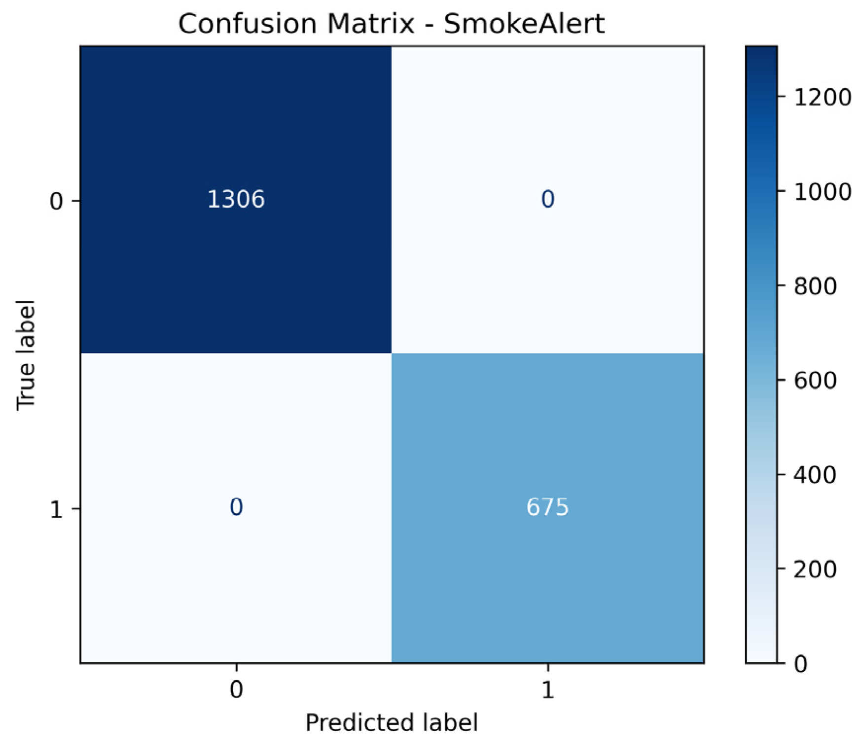
Figure 46.
ROC metric performance results of the sensor fusion system for fire detection.
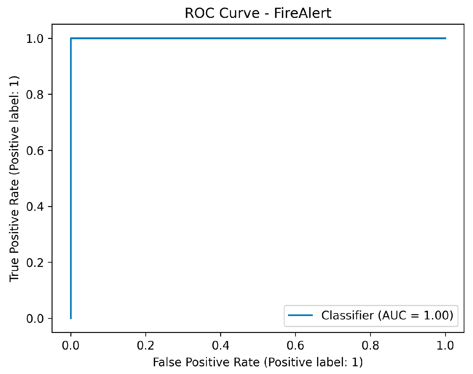
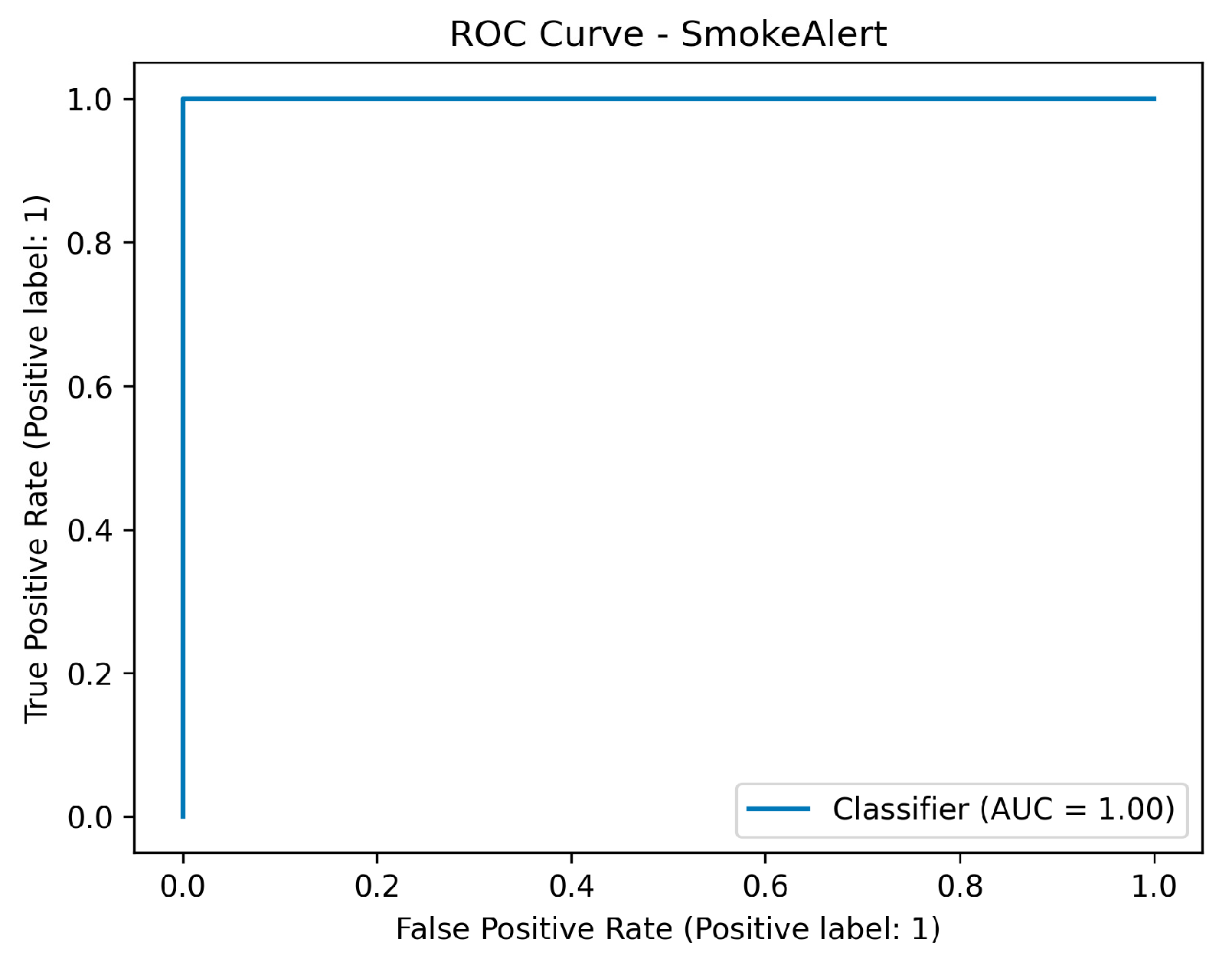
Figure 47.
ROC metric performance results of the sensor fusion system for smoke detection.
4.6. XAI Analysis of the Fused Sensor System
In this step, interpretability analysis was conducted using SHAP The results confirm that the final LightGBM decision-makers place the highest reliance on the derived model probabilities rather than raw sensor inputs alone, validating the strength of the fusion design. For the Fire Alert model, the decision was dominated by Pfire (YOLO’s fire probability), which exhibited a SHAP importance of 0.30, followed by the combined vision probability Pdetection (0.24) and the tabular sensor probability Ptabular (0.14). This hierarchy confirms that visual confirmation is paramount for initiating a fire alarm.
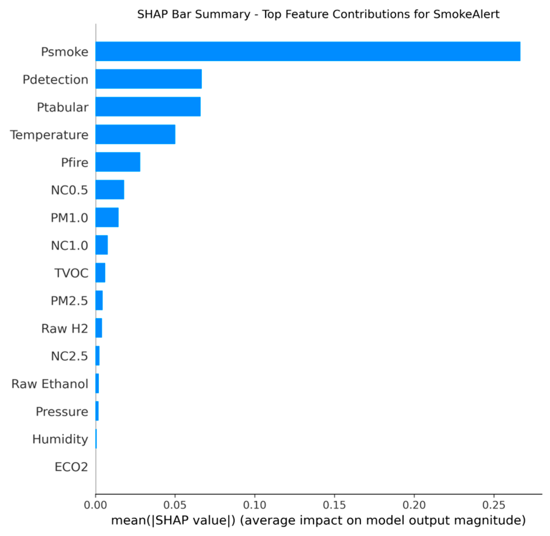
Conversely, the Smoke Alert model was similarly dominated by Psmoke (YOLO’s smoke probability) (0.49), but the relative importance of Ptabular (0.09) closely trailed the general vision probability Pdetection, highlighting the greater necessity of the sensor component for validating the often diffuse and context-sensitive nature of smoke detection. Temperature was the most influential raw sensor feature in both models, providing essential contextual confirmation for thermal events.
Figure 48.
Sensor’s fusion features that contributed the most for fire detection decision-making process.
Figure 48.
Sensor’s fusion features that contributed the most for fire detection decision-making process.

Figure 49.
Sensor’s fusion features that contributed the most for smoke detection decision-making process.
Figure 49.
Sensor’s fusion features that contributed the most for smoke detection decision-making process.
5. Discussion
Taking everything into account, we can conclude that the Explainable Sensor Fusion Framework provided better results than both the Sensor-Only and Vision-Only approaches, in an overall context, because its advantage is that uses the strengths from both worlds, while at the same time addresses their main weaknesses, thus, resulting in a model that provides high robustness and reliability for smoke and fire detection purposes.
More specifically, we noticed that the Sensor-Only System has high numerical accuracy in a controlled environment, but it is quite limited by its lack of spatial generalization, which in turn does not cover all the smoke/fire cases. It is mostly depended on unstable features such as TVOC and Pressure, which makes it unable to confirm the location or presence of a fire event outside its physical range. In contrast, the Vision-Only System (YOLOv8n which achieved the best mAP@0.50 results,) offers excellent spatial coverage and accurate localization of smoke and fire cases, as validated by the application of the LIME XAI method. However, it is still vulnerable to false positives from environmental factors, such as reflections, colored objects, and tiny flames, that could be meaningless or used by machines in the factories or other. Additionally, it operates at a speed that, although it is considered quick, sometimes may risk delays in critical real-time situations (7.5 to 9.5 FPS).
Finally, our designed Fusion System is able to address this trade-off caused by the other two approaches, by using the LightGBM model to efficiently process model confidences, achieving perfect classification (1.0000 Accuracy/F1-score) on the fusion dataset. Then, the conducted SHAP XAI analysis supports this design as well, showing that the final alarm decision depends mainly on the high precision of the visual component (Pfire or Psmoke) for primary detection and then considers the sensor’s readings. On the other hand, the system supports this signal using the Ptabular and temperature features too, to obtain a more robust and essential context.
6. Conclusions
In this work, a robust and interpretable hybrid sensor fusion system for real-time smoke and fire detection was designed and evaluated. To this end, the initial performance analysis of five YOLO nano architectures demonstrated the crucial trade-off in modern object detection: while the latest models like YOLOv12n achieved minimum gains in localization accuracy, their failure to maintain the critical 7 FPS real-time threshold does not make them candidate solutions for immediate deployment. The qualitative XAI analysis using LIME provided the necessary interpretability to justify the final model selection, confirming that YOLOv8n was the optimal choice. Its superior mAP@50 detection accuracy (0.8320) and decent inference-speed (7.5–9.5 FPS) coupled with clean and focused LIME explanations validated its inherent architectural efficiency and minimized the risk of operational latency.
By combining the optimal vision model with a machine learning classifier leveraging environmental sensor data via a weighted product fusion strategy, the integrated system achieved perfect classification (1.0000 for Accuracy, F1-score, and AUC) on the synthesized fusion dataset. This performance proves that the hybrid approach successfully mitigates the single-point failure risks associated with both vision-only systems (vulnerability to visual clutter) and sensor-only systems (zero spatial coverage). Finally, future work includes among others:
- Investigating more sophisticated fusion mechanisms beyond the weighted product approach, such as Attention-based Neural Networks trained end-to-end on the combined sensor and image features, that could potentially yield even higher reliability and resilience to noise.
- The current system’s perfect scores should be validated against a larger, more diverse dataset captured under varying lighting, weather, and obscuration conditions, especially to ensure the model maintains performance against false alarm scenarios (e.g., steam, brightly colored objects, sunsets).
- The YOLO nano models were trained on 20 epochs to test their limits and capabilities. Enriching the models with more epochs and training would lead to even better and promising results.
Author Contributions
Conceptualization, E.D. and P.K.G.; methodology, E.D. and P.K.G.; software, E.D. and P.K.G.; validation, E.D. and P.K.G.; formal analysis, E.D. and P.K.G.; investigation, E.D. and P.K.G.; resources, E.D. and P.K.G.; data curation, E.D. and P.K.G.; writing—original draft preparation, E.D. and P.K.G.; writing—review and editing, E.D. and P.K.G.; visualization, E.D. and P.K.G.; supervision, P.K.G.; project administration, E.D. and P.G.; funding acquisition, P.K.G. All authors have read and agreed to the published version of the manuscript.
Funding
This research received no external funding.
Data Availability Statement
The data presented in this study are available on request from the corresponding author due to privacy and ethical restrictions.
Conflicts of Interest
The authors declare no conflict of interest.
Abbreviations
The following abbreviations are used in this manuscript:
| AI | Artificial Intelligence |
| API | Application Programming Interface |
| DL | Deep Learning |
| NN | Neural Network |
| CNN | Convolutional Neural Network |
| EFB | Exclusive Feature Bundling |
| ESF | Explainable Sensor Fusion |
| FNN | Feedforward Neural Network |
| FPS | Frames per Second |
| HPO | Hyperparameter Optimization |
| IoU | Intersection over Union |
| GOSS | Gradient-based One-Side Sampling |
| GBDT | Gradient Boosting Decision Trees |
| KNC | K-Neighbours Classifier |
| LightGBM | Light Gradient Boosting Machine |
| LIME | Local Interpretable Model-agnostic Explanations |
| mAP | Mean Average Precision |
| ML | Machine Learning |
| MLP | Multilayer Perceptron |
| RNN | Recursive Neural Networks |
| SHAP | SHapley Additive exPlANATIONS |
| SVC | Support Vector Classifier |
| TPE | Tree-structured Parzen Estimator |
| TVOC | Total Volatile Organic Compounds |
| XAI | Explainable Artificial Intelligence |
| XGBoost | eXtreme Gradient Boosting |
| YOLO | You-Only-Look-Once |
References
- Peruzzi, G.; Pozzebon, A.; Van Der Meer, M. Fight Fire with Fire: Detecting Forest Fires with Embedded Machine Learning Models Dealing with Audio and Images on Low Power IoT Devices. Sensors 2023, 23, 783. [Google Scholar] [CrossRef]
- Ali, M.L.; Zhang, Z. The YOLO framework: A comprehensive review of evolution, applications, and benchmarks in object detection. Computers 2024, 13, 336. [Google Scholar] [CrossRef]
- Magdin, M.; Balogh, Z. Comparison classification algorithms and the YOLO method for video analysis and object detection. Sci. Rep. 2025, 15, 25432. [Google Scholar] [CrossRef] [PubMed]
- Hasan, R.H.; Hassoo, R.M.; Aboud, I.S. Yolo versions architecture: Review. Int. J. Adv. Sci. Res. Eng. (IJASRE) 2023, 9, 7. [Google Scholar] [CrossRef]
- Kang, S.; Hu, Z.; Liu, L.; Zhang, K.; Cao, Z. Object detection YOLO algorithms and their industrial applications: Overview and comparative analysis. Electronics 2025, 14, 1104. [Google Scholar] [CrossRef]
- Mela, J.L.; García Sánchez, C. Yolo-based power-efficient object detection on edge devices for USVs. J. Real-Time Image Process. 2025, 22, 108. [Google Scholar] [CrossRef]
- Polenakis, I.; Sarantidis, C.; Karydis, I.; Avlonitis, M. A comparative study of YOLO algorithm variants. Signals 2025, 6, 60. [Google Scholar] [CrossRef]
- Zhou, Y.; Guo, Z.; Dong, Z.; Yang, K. TensorRT implementations of model quantization on edge SoC. In Proceedings of the 2023 IEEE 16th International Symposium on Embedded Multicore/Many-core Systems-on-Chip (MCSoC), Singapore, 18–21 December 2023; pp. 486–493. [Google Scholar] [CrossRef]
- Feng, H.; Mu, G.; Zhong, S.; Zhang, P.; Yuan, T. Benchmark analysis of YOLO performance on edge intelligence devices. Cryptography 2022, 6, 16. [Google Scholar] [CrossRef]
- Han, B.-G.; Lee, J.-G.; Lim, K.-T.; Choi, D.-H. Design of a scalable and fast YOLO for edge-computing devices. Sensors 2020, 20, 6779. [Google Scholar] [CrossRef]
- Humes, E.; Navardi, M.; Mohsenin, T. Squeezed Edge YOLO: Onboard object detection on edge devices. arXiv 2023, arXiv:2312.11716. [Google Scholar] [CrossRef]
- Li, J.; Ye, J. Edge-YOLO: Lightweight infrared object detection method deployed on edge devices. Appl. Sci. 2023, 13, 4402. [Google Scholar] [CrossRef]
- Roshan, K.; Zafar, A. Utilizing XAI technique to improve autoencoder based model for computer network anomaly detection with shapley additive explanation (SHAP). arXiv 2021, arXiv:2112.08442. [Google Scholar] [CrossRef]
- Nguyen, H.T.T.; Cao, H.Q.; Nguyen, K.V.T.; Pham, N.D.K. Evaluation of Explainable Artificial Intelligence: SHAP, LIME, and CAM. In Proceedings of the FPT AI Conference 2021, Ha Noi, Viet Nam, 6–7 May 2021. [Google Scholar]
- Dieber, J.; Kirrane, S. Why model why? Assessing the strengths and limitations of LIME. arXiv 2020, arXiv:2012.00093. [Google Scholar] [CrossRef]
- Abadi, M.; Barham, P.; Chen, J.; Chen, Z.; Davis, A.; Dean, J.; Devin, M.; Ghemawat, S.; Irving, G.; Isard, M.; et al. TensorFlow: A system for large-scale machine learning. arXiv 2016, arXiv:1605.08695. [Google Scholar] [CrossRef]
- Chicho, B.T.; Bibo Sallow, A. A comprehensive survey of deep learning models based on Keras framework. J. Soft Comput. Data Min. 2021, 2, 49–62. [Google Scholar] [CrossRef]
- Pedregosa, F.; Varoquaux, G.; Gramfort, A.; Michel, V.; Thirion, B.; Grisel, O.; Blondel, M.; Prettenhofer, P.; Weiss, R.; Dubourg, V.; et al. Scikit-learn: Machine Learning in Python. J. Mach. Learn. Res. 2011, 12, 2825–2830. [Google Scholar] [CrossRef]
- Stoltzfus, J.C. Logistic regression: A brief primer. Acad. Emerg. Med. 2011, 18, 1099–1104. [Google Scholar] [CrossRef]
- Dhananjay, B.; Sivaraman, J. Analysis and classification of heart rate using CatBoost. Biomed. Signal Process. Control 2021, 68, 102610. [Google Scholar] [CrossRef]
- Suyal, M.; Goyal, P. A review on analysis of K-Nearest Neighbor classification machine learning algorithms based on supervised learning. Int. J. Eng. Trends Technol. 2022, 70, 43–48. [Google Scholar] [CrossRef]
- Valkenborg, D.; Rousseau, A.J.; Geubbelmans, M.; Burzykowski, T. Support vector machines. Am. J. Orthod. Dentofac. Orthop. 2023, 164, 754–757. [Google Scholar] [CrossRef] [PubMed]
- Priyam, A.; Gupta, R.K.; Srivastava, S. Comparative analysis of decision tree classification algorithms. Int. J. Comput. Sci. Eng. 2013, 3, 334–337. [Google Scholar]
- Kulkarni, V.Y.; Sinha, P.K. Random forest classifiers: A survey and future research directions. Int. J. Adv. Comput. 2013, 36, 1144–1153. [Google Scholar]
- Torlay, L.; Perrone-Bertolotti, M.; Thomas, E.; Baciu, M. Machine learning–XGBoost analysis of language networks to classify patients with epilepsy. Brain Inform. 2017, 4, 159–169. [Google Scholar] [CrossRef]
- Gan, M.; Pan, S.; Chen, Y.; Cheng, C.; Pan, H.; Zhu, X. Application of the machine learning LightGBM model to the prediction of the water levels of the lower Columbia River. J. Mar. Sci. Eng. 2021, 9, 496. [Google Scholar] [CrossRef]
- Priyam, A.; Gupta, R.K.; Srivastava, S. Comparison of the CatBoost Classifier with other classification algorithms. Int. J. Comput. Appl. 2017, 11, 738–748. [Google Scholar]
- Cao, Y. An MLP classifier for prediction of HBV-induced liver cirrhosis using routinely available clinical parameters. Dis. Markers 2013, 35, 653–660. [Google Scholar] [CrossRef] [PubMed]
- Mishra, C.; Gupta, D.L. Deep machine learning and neural networks: An overview. IAES Int. J. Artif. Intell. (IJ-AI) 2017, 6, 66–73. [Google Scholar] [CrossRef]
- Singh, M.; Akula, A. A comparative study of YOLO-V5 variants performance for object detection in thermal infrared images. In Proceedings of the 2024 IEEE 5th India Council International Subsections Conference (INDISCON), Virtual, India, 13–15 December 2024; pp. 1–6. [Google Scholar] [CrossRef]
- Wang, J.; Qi, Z.; Wang, Y.; Liu, Y. A lightweight weed detection model for cotton fields based on an improved YOLOv8n. Sci. Rep. 2025, 15, 457. [Google Scholar] [CrossRef]
- Gong, Y.; Ding, W.; Huang, N.; Li, T.; Zhou, J. Improved YOLOv10n model for enhanced cotton recognition. Smart Agric. Technol. 2025, 12, 101209. [Google Scholar] [CrossRef]
- He, J.; Wang, W. Improved YOLOv10 model for small target UAV detection. Ain Shams Eng. J. 2025, 16, 103787. [Google Scholar] [CrossRef]
- Gao, L.; Cao, H.; Zou, H.; Wu, H. DMN-YOLO: A robust YOLOv11 model for detecting apple leaf diseases in complex field conditions. Agriculture 2025, 15, 1138. [Google Scholar] [CrossRef]
- Khanam, R.; Hussain, M. YOLOv11: An overview of the key architectural enhancements. arXiv 2024, arXiv:2410.17725. [Google Scholar] [CrossRef]
- Tian, Y.; Ye, Q.; Doermann, D. YOLOv12: Attention-Centric Real-Time Object Detectors. arXiv 2025, arXiv:2502.12524. [Google Scholar] [CrossRef]
- Bakir, C.; Gezer, A. Real-Time Automatic Detection of Nutrient Deficiency in Lettuce Plants With New YOLOV12 Model. J. Sens. 2025, 2025, 1. [Google Scholar] [CrossRef]
- Lundberg, S.; Lee, S.-I. A unified approach to interpreting model predictions. In Proceedings of the 31st International Conference on Neural Information Processing Systems (NIPS 2017), Long Beach, CA, USA, 4–9 December 2017; pp. 3593–3602. [Google Scholar] [CrossRef]
- Ribeiro, M.T.; Singh, S.; Guestrin, C. “Why should I trust you?”: Explaining the predictions of any classifier. In Proceedings of the 22nd ACM SIGKDD International Conference on Knowledge Discovery and Data Mining (KDD), San Francisco, CA, USA, 13–17 August 2016; pp. 1135–1144. [Google Scholar] [CrossRef]
- Akiba, T.; Sano, S.; Yanase, T.; Ohta, T.; Koyama, M. Optuna: A next-generation hyperparameter optimization framework. In Proceedings of the 25th ACM SIGKDD International Conference on Knowledge Discovery & Data Mining (KDD), Anchorage, AK, USA, 4–8 August 2019; pp. 2623–2631. [Google Scholar] [CrossRef]
- Dibra, E. Explainable Smoke And Fire Detection System [Code Repository]; GitHub. 2025. Available online: https://github.com/EndriDibra/Explainable_Smoke_And_Fire_Detection_System/tree/main (accessed on 1 December 2025).
- Blattmann, S. Smoke Detection Dataset [Dataset]; Kaggle. 2023. Available online: https://www.kaggle.com/datasets/deepcontractor/smoke-detection-dataset (accessed on 1 December 2025).
- Menon, G. Fire and Smoke (Roboflow) [Dataset]; Kaggle. 2023. Available online: https://www.kaggle.com/datasets/gautamrmenon/fire-and-smoke-roboflow (accessed on 1 December 2025).
- Mark, J. Where There’s Fire, There’s Smoke. The New York Times, Opinion. 2017. Available online: https://www.nytimes.com/2017/09/08/opinion/where-theres-fire-theres-smoke.html.
- Egan, C. Wildfire Smoke and Your Health. Steinbach First Aid. 2025. Available online: https://steinbachfirstaid.com/wildfire-smoke-and-your-health/.
- Smoke. Wikipedia, The Free Encyclopedia. Available online: https://en.wikipedia.org/wiki/Smoke (accessed on 1 December 2025).
- iStockphoto. Fire in the City Overview. Getty Images. Available online: https://media.istockphoto.com/id/494853349/photo/fire-in-the-city-overview.jpg?s=612x612&w=0&k=20&c=J9w2-ys_Y79cblBJJgw9Ybtw2QrL4ZiSLf39jE77pW0= (accessed on 1 December 2025).
- ABC News. Campbellfield Factory Fire Sends Smoke Over Melbourne’s North. ABC News. 2019. Available online: https://www.abc.net.au/news/2019-04-05/campbellfield-factory-fire-sends-smoke-over-melbournes-north/10973650.
- Vecteezy. A Large Industrial Plant with a Large Fire in the Background. Vecteezy. Available online: https://www.vecteezy.com/video/50735718-a-large-industrial-plant-with-a-large-fire-in-the-background (accessed on 1 December 2025).
- Vecteezy. A Large Industrial Plant with Lots of Smoke Coming out of it. Vecteezy. Available online: https://www.vecteezy.com/video/50735570-a-large-industrial-plant-with-lots-of-smoke-coming-out-of-it (accessed on 1 December 2025).
- IMEC Technologies. Causes of Fires in Manufacturing Plants. IMEC Technologies. 2020. Available online: https://www.imectechnologies.com/2020/12/15/causes-of-fires-in-manufacturing-plants/.
- Millennium Fire Protection. Most Common Causes of Factory Fires. Millennium Fire Protection. Available online: https://www.m-f-p.co.uk/news/most-common-causes-of-factory-fires/ (accessed on 1 December 2025).
Figure 9.
Detection and Bounding boxing of smoke/fires regions with YOLOv5nu.
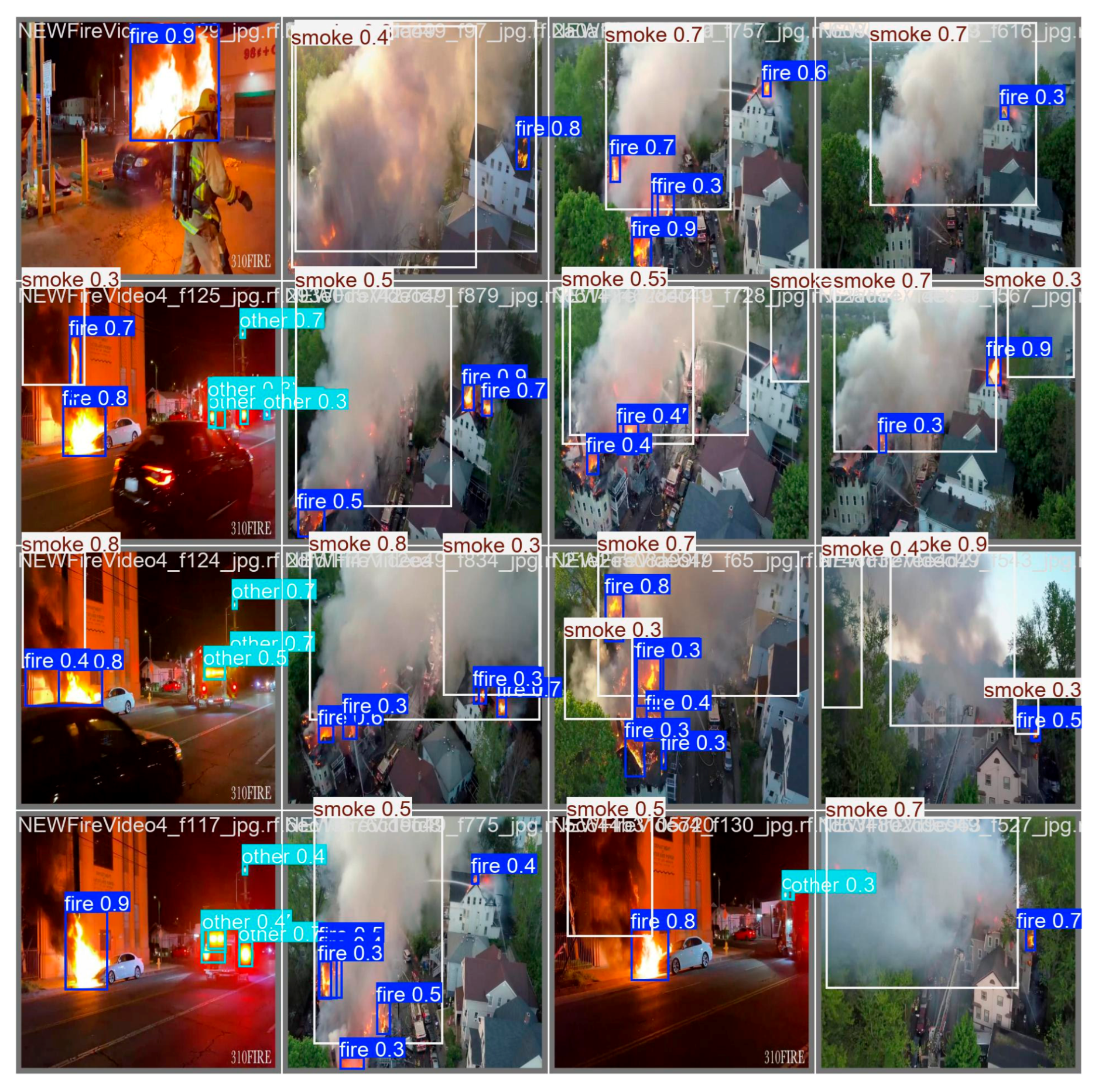
Figure 16.
Detection and Bounding boxing of smoke/fires regions with YOLOv8n.

Figure 23.
Detection and Bounding boxing of smoke/fires regions with YOLOv10n.
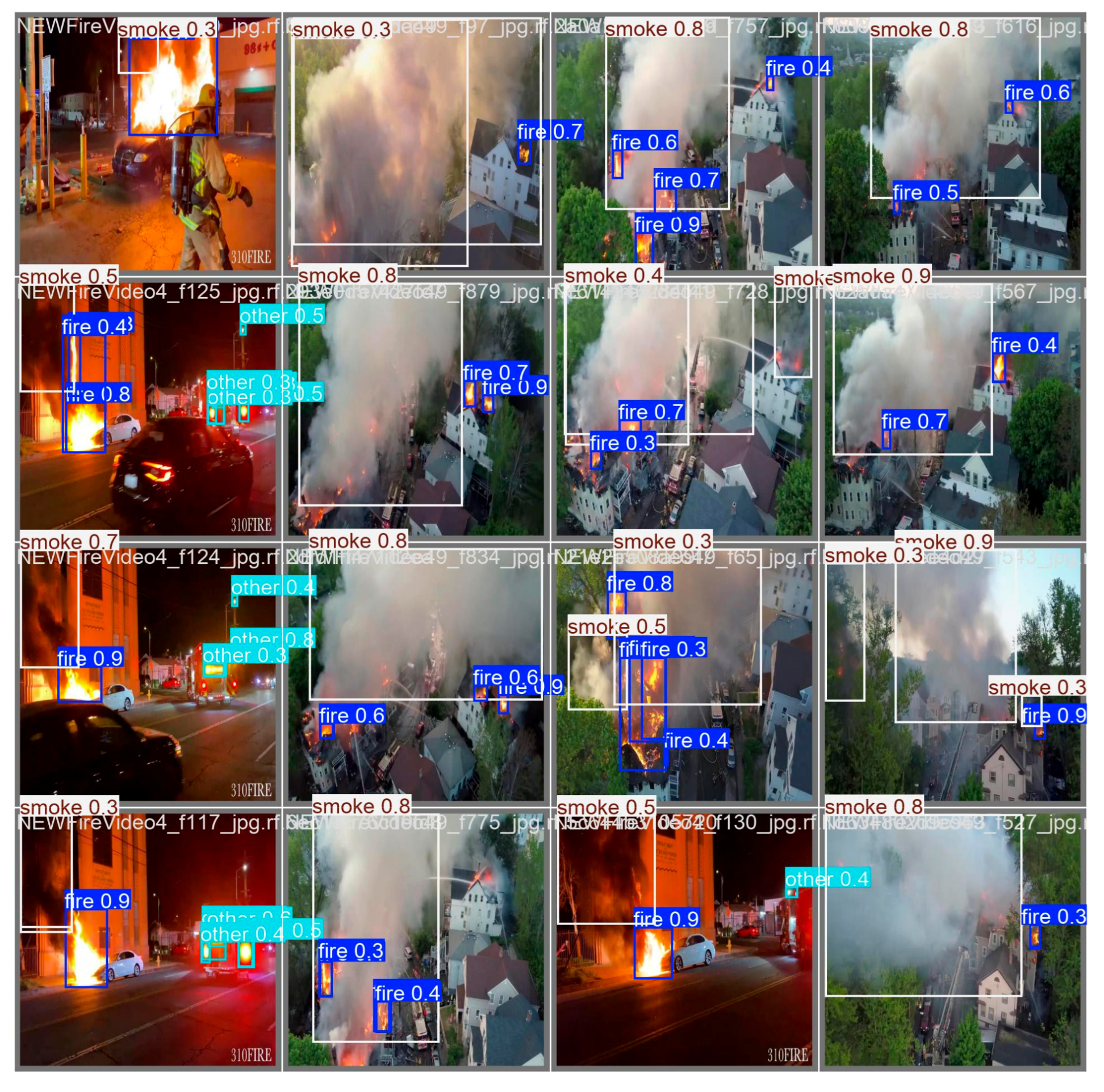
Figure 30.
Detection and Bounding boxing of smoke/fires regions with YOLOv11n.
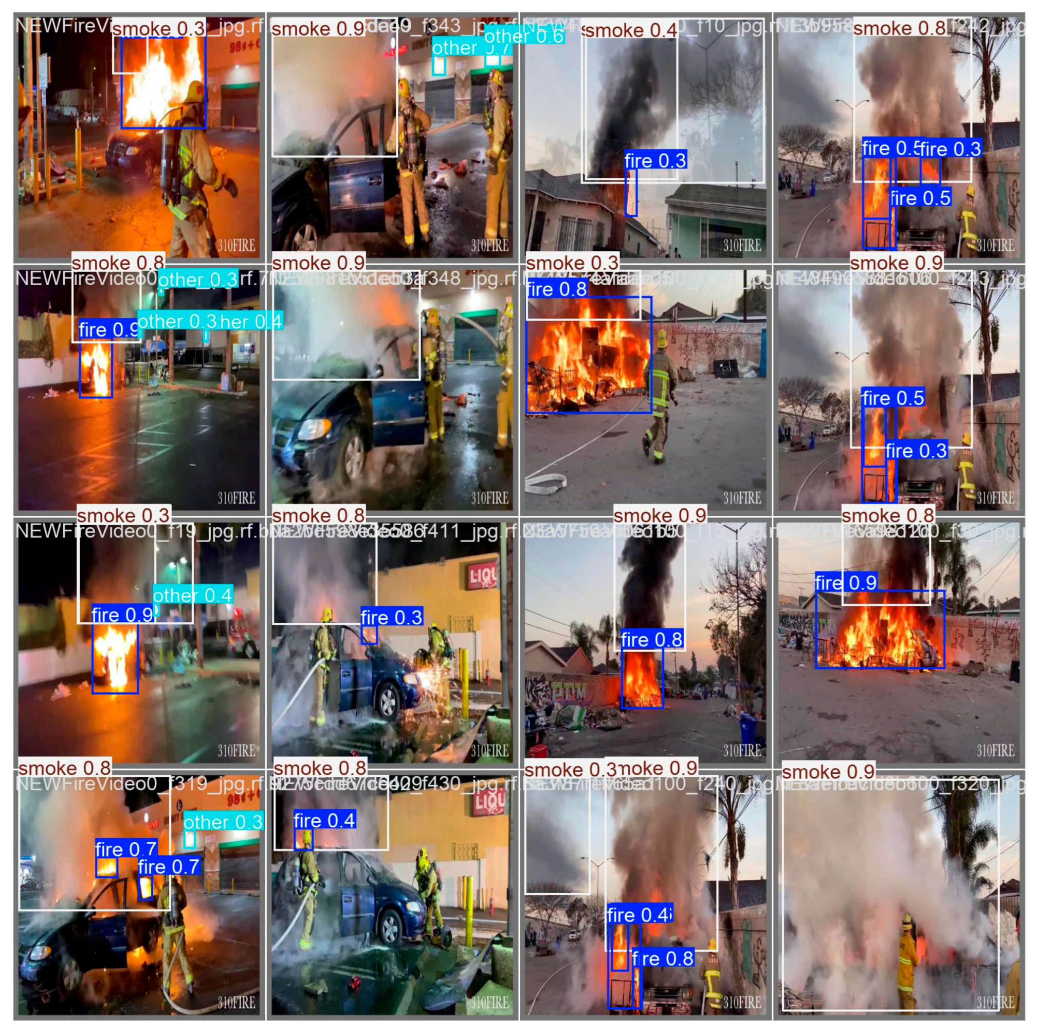
Figure 37.
Detection and Bounding boxing of smoke/fires regions with YOLOv12n.
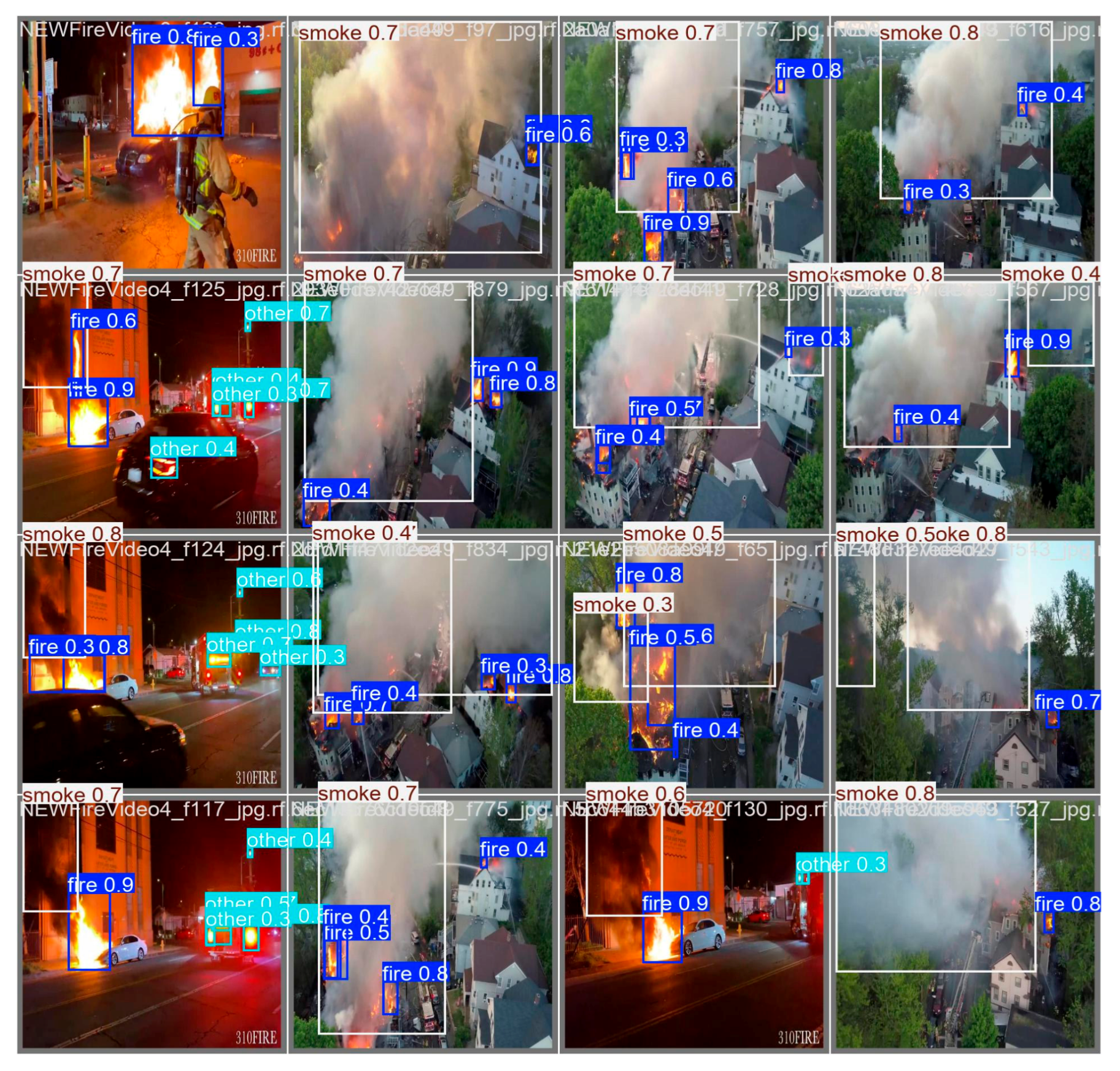
Table 1.
Performance metrics of the ML and DL models.
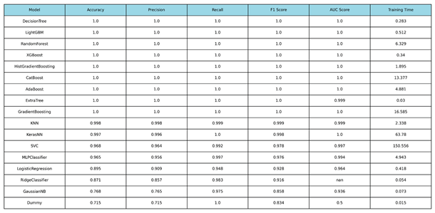 |
Table 2.
Features’ importance contribution on model’s final decision-making process
 |
Disclaimer/Publisher’s Note: The statements, opinions and data contained in all publications are solely those of the individual author(s) and contributor(s) and not of MDPI and/or the editor(s). MDPI and/or the editor(s) disclaim responsibility for any injury to people or property resulting from any ideas, methods, instructions or products referred to in the content. |
© 2025 by the authors. Licensee MDPI, Basel, Switzerland. This article is an open access article distributed under the terms and conditions of the Creative Commons Attribution (CC BY) license (http://creativecommons.org/licenses/by/4.0/).
Copyright: This open access article is published under a Creative Commons CC BY 4.0 license, which permit the free download, distribution, and reuse, provided that the author and preprint are cited in any reuse.


