
Submitted:
17 December 2025
Posted:
18 December 2025
You are already at the latest version
Abstract
Diatoms are key primary producers and sensitive indicators in polar freshwater ecosystems, responding rapidly to environmental change. This study investigates diatom species richness and the influence of environmental variables in fourteen coastal lakes on King George and Horseshoe Islands in the maritime Antarctic. Water and surface sediment samples collected in 2017, 2019, and 2020 were analyzed using light and scanning electron microscopy, revealing 86 diatom species and genera across all lakes except Lake 5. King George Island exhibited higher species richness, with frequent occurrences of Planothidium lanceolatum, Achnanthidium dolomiticum, Fragilaria capucina and Nitzschia homburgiensis. On Horseshoe Island, common taxa included Achnanthes, Achnanthidium, Fragilaria, Nitzschia, Navicula, and Gomphonema. Among the previously measured water chemistry variables, HCO3- (ρ = 0.78, p = 0.005) and K+ (ρ = 0.69, p = 0.019) showed the strongest positive correlations with diatom species richness. Major ions and nutrients exhibited moderate relationships with DO, salinity, and pH. In contrast, temperature and trace metals displayed weak or negligible correlations, suggesting indirect influences on diatom diversity. These findings demonstrate that diatom communities in the Maritime Antarctic lakes are highly diverse and are strongly shaped by variations in water chemistry, underscoring the ecological sensitivity of these freshwater ecosystems.
Keywords:
diatoms
; morphology
; maritime antarctic
; King George Island
; Horseshoe Island
; environmental drivers
; lake
; pond
; light microscopy
; scanning electron microscopy
1. Introduction
Diatoms (Bacillariophyta) are a major group of microalgae in aquatic systems, dominating the water columns in rivers and oceans. As primary producers, diatoms are responsible for approximately 25% of global and 50% of marine primary production, which exceeds the amount of oxygen produced by all rainforests [1]. Through this production, diatoms contribute to carbon fixation, holding around 45% of marine CO₂ [2]. Moreover, diatoms provide the main dietary source for aquatic feeders, thereby representing a major component of aquatic food webs, particularly in the Antarctic polar regions. Considering this key role, the identification of diatoms in Antarctic lakes is important for understanding how these communities will respond to extreme conditions and the multiple impacts of stressors such as warming, climate change and human-caused stressors.
In Antarctica, diatoms are very common and important primary producers in both marine and freshwater systems where they participate in nutrient cycling and food webs. Phytoplankton productivity is also important for regulating atmospheric carbon and methane as the lakes on King George Island were found to be a net carbon dioxide sink on an annual basis [3]. High variability of bacterial communities among different lakes suggested strong spatial differences among lakes in the Maritime Antarctic [4]. Previous studies have documented different diatom species in some regions, especially on King George Island and other South Shetland Islands [5,6,7]. These studies have indicated that environmental factors such as temperature, salinity, pH, nutrients, and even exposure to darkness and glaciers are strong determinants of diatom composition [8,9,10]. Changes in temperature and salinity may affect the biochemical properties of some diatom species such as Nitzschia lecointei [11]. Similarly, metal bioavailability is also important because metals play key roles as cofactors in many metabolic reactions, thereby affecting growth rates [12]. For instance, manganese (Mn) and iron (Fe) are essential for enzymes used in photosynthesis and detoxification mechanisms, while molybdenum (Mo) is a key element in the nitrogen cycle [13,14,15]. Additionally, cobalt (Co), copper (Cu) and zinc (Zn+2) affect growth of the marine diatoms, highlighting how metal co-limitation is crucial for enzyme catalysis, protein structure and metabolism, especially in high-nutrient low-chlorophyll (HNLC) regions as Fe is a limiting-factor [16,17]. In addition to metal requirements, macronutrients, micronutrients, and ions are essential for algal growth [18]. For instance, diatoms require silica (Si) for cell wall formation, nitrogen (N) and phosphorus (P) for biochemical synthesis, sodium (Na+) for cell division, and calcium (Ca+2), magnesium (Mg+2), sulfate (SO₄-2), nitrate (NO3-), potassium (K+), and bicarbonate (HCO₃⁻) for other physiological processes [19]. A recent study showed that chlorophyll-a (Chl-a) concentrations have a strong correlation with ammonium (NH₄⁺) and NO3- in the Maritime Antarctic, suggesting that nutrients, as well as key cations and anions, play an important role in phytoplankton growth [18].
On the other hand, it has been shown that six benthic diatom species from the Antarctic Peninsula can acclimate to fluctuating temperature, salinity and light levels broader than their actual conditions, suggesting high flexibility in coping with environmental change [10]. Together, these studies emphasize that Antarctic diatoms are strongly influenced by changing of environmental conditions, yet they also exhibit some plasticity to cope with ongoing and possible future stressors.
Despite all these previous studies, our knowledge of Antarctic freshwater diatom diversity remains incomplete. Many lakes and ponds across the Antarctic region have yet to be studied systematically. Although some new diatom species have been identified over the past few decades through morphological or molecular approaches [5,6,20,21], most available records are still limited. While molecular methods such as metabarcoding are increasingly applied to samples to improve taxonomic knowledge [4], there are still some debates regarding the preservation of deoxyribonucleic acid (DNA) and Ribonucleic acid (RNA) in remote field expeditions and ongoing isolation and sequencing procedures. Consequently, morphological identification by light microscopy (LM) and scanning electron microscopy (SEM) seems to be more reliable and applicable approach for characterization of diatom communities in these harsh environments. Therefore, to contribute to our current knowledge gaps about diatom diversity, we examined the diatom species of lakes and ponds from King George Island (62°S) in the South Shetland Islands and Horseshoe Island (67°S) further south on the Antarctic Peninsula. Using light and scanning electron microscopy, we examined diatom distribution and richness and discussed how physicochemical parameters and key nutrients, metals and ions can affect diatom variability across sampling sites, also considering possible future climate effects.
2. Materials and Methods
2.1. Study Site
Sampling of water, filters and sediments from lakes and ponds in the Maritime Antarctic was performed in three field campaigns; first in February-March 2017, second in January 2019 on King George Island and third in February 2020 on Horseshoe Island (Table 1).
Samples were collected from nine lakes (L1-L6, HS1, HS2, SK), three ponds (P1-P3) and two organic ponds (OP1, OP2) (Figure 1, Table 1). Only OP2 was located on Ardley Island section of King George, while the others were from the Fildes Peninsula (Figure 1a,f). The sampling locations were studied previously to understand methane and carbon dioxide cycles and also lithological controls on lake water chemistry (Olgun et al., 2024; Thalasso et al., 2022). In the second campaign, water and filter samples were taken from five of these lakes including Uruguay (L1), Kitiesh (L2), L4, P1, OP2 (Table 1), while no sediment samples were taken in 2019. The third campaign in 2020 on Horseshoe Island (Figure 1b,) was done as part of the Turkish Antarctic Expedition (TAE) and water, filter and sediment samples were collected from Horseshoe-1 (HS1), Horseshoe-2 (HS2) and Skua Lake (SK) (Figure 1e,h,g,i).
2.2. Sampling
Samples from L2 on King George Island were collected from a single location at the center of the lake (-12 m water depth) using a small boat (Figure 1c). The L2 water sample was collected with a 2.2 L Van Dorn water sampler and the sediment sample with a sediment grab (Figure 1d). Due to harsh weather conditions, samples from other lakes were collected from a single sampling location in the littoral zone of the lakes and ponds. No sediment sample was taken from L1 in either 2017 or 2019. All sediment samples were stored in plastic bags and kept cool at a temperature of +4ºC.
100 mL of water samples were used for morphological species identification. To preserve the samples, 0.5 mL of Merck® Lugol's iodine solution was added per 50 mL of sample. The samples were then covered with aluminum foil to protect from sunlight and were stored in the refrigerator +4ºC.
Filter samples were collected by filtering 2370 mL of surface water from L1, 4870 mL from L2, 1500 mL from OP2, 200 mL from HS1 and HS2 and 150 mL of SK through Whatman® polycarbonate (PC) filters with 0.22 µm pore size and 47 mm diameter. Filter sample of L1 was used for phytoplankton species determination in SEM analyses as there were no sediment samples from L1. After the filtration process, the filters were carefully folded and placed in an aluminum foil and then stored at a temperature of -20ºC.
Water parameters including pH, dissolved oxygen (DO), temperature, conductivity, salinity and total dissolved solids (TDS) were measured in six lakes and five ponds on King George Island in 2017 using a multiparameter probe (HI 9828, Hanna Instruments, Mexico) (Table 2). Chl-a concentrations were measured using an Ultraviolet–visible (UV-Vis) spectrophotometry in the Chilean Escudero Station (Table 2) (Thalasso et al., 2022). Oxidation-reduction potentials (ORP) of five of these lakes on King George were measured in 2019 (Table 2). The measured parameters were not identical in each lake or each year, as the samplings were done in different campaigns. Indicated metal, nutrient and ion concentrations in Table 2 are based on ion chromatography and inductively coupled plasma mass spectrometer (ICP-MS) data obtained in a previous study (Olgun et al., 2024).
2.3. Morphological Analyses with LM and SEM
Each diatom group was assigned to one of the diatom taxa based on its valve symmetry, septa, striae, raphe system, and valve shapes. The presence or absence of raphe and its position was the first step for distinguishing between different diatom species. Further identification of raphid diatoms was performed by examining the characteristics of the raphe itself, such as its form, curvature, and number of striae. The position of the raphe on the valve can also vary from species to species. For example, it may occur at the edges, on the side or offset from the center of the valve. In cases where a raphe was not visible, the septa were used for identification. However, a morphology-based identification approach alone may be insufficient for some species because of high morphological similarities and some blurred microscopic images.
For LM analysis, both water and sediment samples were used. For the sediment samples, one gram of bulk wet sediment was diluted in 50 ml of distilled water and vortexed for 45 seconds at 1600 rpm. No acid digestion using hydrogen peroxide or hydrochloric acid was applied to samples in order to avoid the loss of additional information belonging to other microorganisms such as coccolithophorids, if present. The slides were covered with Merck® immersion oil and examined under 100x objective lens. An Ivymen System light microscope equipped with a Zeiss Plan-Apochromat 100x immersion lens was used. The images were generated with a Canon EOS 500D digital camera equipped with Canon EOS Utility software (Canon Inc., Tokyo, Japan).
SEM image analyses of diatom frustules were conducted with sediment samples, as the number of frustules in the water samples was insufficient and diatom abundance was very low. For L1, the filter collected in 2019 was used, since there were no available sediment samples from this lake. For SEM analysis, one gram of bulk sediment was diluted in 50 mL distilled water and vortexed at 1600 rpm for 45 seconds. The sediment suspension was then filtered through a Whatman® polycarbonate filter (0.22 µm pore size). Filters were placed in Petri dishes and dried for five hours in an incubator at 70 ºC before SEM examination. A small portion of each filter (approximately one centimeter square) was cut, mounted on aluminum stubs, and coated with gold. SEM analyses were conducted using a Zeiss EVO 10 scanning electron microscope. The relative abundance of each diatom taxa observed in the sediment samples (except for L1) was categorized as follows: very rare (vr): 1-5 shells, rare (r): 5-10 shells, frequent (f): 10-30 shells, and common (c) >30 shells (Table S1).
3. Results
This A total of 86 diatom species and genera were recorded from King George and Horseshoe Islands. A summary of the diatom species encountered in each lake is listed with their relative abundances in Supplementary Table (Table S1). Representative LM and SEM images showing the morphology of the recorded diatoms are presented in Figure 3. The most frequently observed species across the studied lakes were Planothidium lanceolatum, Achnanthidium dolomiticum, Fragilaria capucina, Nitzschia homburgiensis, Planothidium delicatulum, Pinnularia brebissonii and Craticula pseudocitrus (Figure 2).
Figure 2.
The ten most widespread diatom species identified in lakes and ponds of King George and Horseshoe Islands in the Maritime Antarctic.
Figure 2.
The ten most widespread diatom species identified in lakes and ponds of King George and Horseshoe Islands in the Maritime Antarctic.
The sizes of diatom valves varied, ranging from approximately 10 μm to 40 μm in length and from 2 μm to 15 μm in width. Pinnularia divergens and Achnanthes sp. were the largest species encountered, with approximately 10-15 μm in length (Figure 3, pic. 1, 43). In contrast, Achnanthidium cf. dolomiticum and Diadesmis sp. species were the smallest, ranging from 10 μm in length (Figure 3, pic. 19, 39). Most identified taxa were pennate diatoms, except for a few centric diatoms found in L1 and L6 in Fildes Peninsula, and in OP2 on Ardley Island (Figure 3, pic. 84).
Figure 3.
Examples of diatom species in King George and Horseshoe Islands. 1. Pinnularia divergens in L4 2. Pinnularia subcapitata var. subrostrata in OP2 3. Pinnularia cf. rhombarea in OP1 4. Pinnularia microstauron var. elongata in P3 5. Pinnularia subsolaris in OP1 6. Pinnularia brebissonii in LM in OP1 and SEM in L6 7. Pinnularia cf. quadratarea in P2 8. Pinnularia sp. in P2 9. Fragilaria cf. capucina in P1 10. Fragilaria sp. in OP2 11. Pinnularia borealis in OP1 12. Pinnularia cf. subantarctica in OP2 13. Fragilaria cf. nanana in P1 14. Fragilaria cf. rumpens in OP1 15. Fragilaria cf. fragilarioides in P2 16. Fragilaria cochabambina in P3 17. Fragilaria capucina in OP2 18. Fragilaria sp. in L3 19. Achnanthidium cf. dolomiticum in OP2 20. Achnanthidium cf. minutissimum in P2 21. Achnanthidium nanum in L2 22. Achnanthidium cf. australexiguum in L2 23. Achnanthidium spp. in P1 24. Achnanthidium cf. reimeri in L6 25. Achnanthidium sp. in OP2 26. Humidophilia sp. in OP2 27. Humidophilia arcuata var. parallela in P2 and P3 28. Planothidium lanceolatum in P2 29. Planothidium cf. frequentissimum in L4 30. Planothidium delicatulum in L4 31. Planothidium cf. subantarcticum in L3 32. Planothidium biporomum in L3 33. Planothidium cryptolanceolatum in P3 34. Planothidium victorii in L4 35. Planothidium incuriatum in L4 36. Planothidium sp. in L6 37. Diadesmis tabellariaeformis in P3 38. Diadesmis cf. faurei in P3 39. Diadesmis sp. in P1 40. Craticula spp. in OP2 41. Craticula pseudocitrus in L6 42. Achnanthes cf. sinaensis in P1 43. Achnanthes sp. in L4.
Figure 3.
Continue: 44. Achnanthes taylorensis in OP1 45. Nitzschia spp. in OP1 46. Nitzschia homburgiensis in OP1 47. Nitzschia capitellata in L3 48. Gomphonema micropus in OP2 49. Gomphonema cf. sarcophagus in OP2 50. Gomphonema angustatum in OP2 51. Gomphonema sp. in L2 52. Gomphonema gracile in L4 53. Gomphonema duplipunctatum in L4 54. Gomphonema subclavatum in L4 55. Gomphonella sp. in L2 56. Navicula cf. rhynchotella in P2 57. Navicula libonensis in L6 58. Navicula sp. in L6 59. Navicula gregaria in L6 60. Navicula cf. slesvicensis in L6 61. Navicula cf. trilatera in L4 62. Navicula cf. veneta in P1 63. Diatomella balforiana in L2 64. Eunotia sp. in L4 65. and 80. Placoneis explanata in OP1 and OP2 66. Placoneis paraelginensis in L6 67. Sellaphora sp. in L2 68. Staurosirella sp. in L4 69. Luticola cf. muticopsis in OP2 70. Frustulia sp. in P3 71. Luticola cf. permuticopsis in P3 72. Luticola sp. in L2 73. Eunotia sp. in P3 74. Psammothidium lacustre in P3 75. Psammothidium helveticum in L3 76. Psammothidium cf. acidoclinatum in L6 77. Psammothidium cf. confusoneglectum in L2 78. Psammothidium sp. in P2 79. Stauroneis subgracilis in P1 81. Tabellaria flocculosa in OP2 82. Halamphora sp. in L4 83. Adlafia sp. in P1 84. Unidentified centric diatoms in OP2, L1, P1 respectively 85. Thalassionema nitzschioides in P1 86. Halamphora coraensis in L4 87. Stauroforma inermis in P3 88. Chamaepinnularia hassiaca in P2 89. Chamaepinnularia cf. frisca in OP2 90. Planothidium sp. and Psammothidium cf. confusoneglectum in L2 91. Planothidium delicatulum, Fragilaria sp. and Gomphonema sp. (From left to right) in OP2 92. Unidentified centric and pennate diatoms in L6 93. Fragilaria sp. and Planothidium sp. in P2.
Figure 3.
Continue: 94. Diatom species, unidentified genus 95. Diatom species, unidentified genus, frustules in girdle view 96. Coccolithophoride sp. (non-diatom) in L2 97. Non-phytoplankton species, unidentified genus in L1 and L6 98. Abnormal forms of diatoms in the water and sediment samples respectively Fragilaria capucina in OP2 (the first three figures), Planothidium victorii in L4, Craticula pseudocitrus in L3.
The relative abundance of each diatom species in the samples was generally very rare (1-5 frustules) or rare (5-15 frustules) (Table S1). The most diatom-rich sites were L4 (31 species), OP2 (28 species), and L6 (26 species) in King George Island. Only a few diatoms were found in L1 (four species) in the Fildes Peninsula due to a lack of sediment samples for this lake. Horseshoe Island lakes also showed limited diatom species richness, with a maximum of four species in HS2. Interestingly, no diatoms could be detected in the L5 (West Lake) in Fildes Peninsula on King George Island, both in water and the sediment samples.
The correlations between diatom species richness and environmental parameters exhibited weak to strong positive relationships. HCO₃⁻ (Spearman ρ = 0.78, p = 0.005) and K+ (Spearman ρ = 0.69, p = 0.019) had strong positive and significant correlations with diatom species richness, while DO (Spearman ρ = 0.56, p = 0.039) exhibited a moderate but significant positive relationship (Figure 4). Most parameters such as salinity, Na+, Ca+2, Mg+2, SO₄-2, NO3-, and Si showed moderate positive but non-significant correlations (Figure 4). Conversely, temperature, Fe, Co, and Zi+2 represented weak or negligible correlations (Figure 4).
4. Discussion
Authors All of the studied maritime Antarctic lakes contained diatoms, except for Lake L5 on King George Island (Table S1). Most of the identified species matched to those previously reported from King George Island, including Pinnularia subantarctica, Pinnularia borealis, Planothidium lanceolatum, Fragilaria capucina, and Nitzschia capitellata [22,23]. Microscopic analyses revealed that the lakes on King George Island included higher numbers of diatom species than those on Horseshoe Island, which lies about 600 km farther south (Table S1). The difference between the diatom species richness across the two studied islands may be related to the considerably lower temperatures in Horseshoe Island samples, which reached a maximum of only 2.8oC (Table 2). In addition, factors such as lithology of the lake catchment area, sea spray inputs, and ornithogenic activity appear to impact water biogeochemistry, and consequently, the diatom species richness observed in the lakes on King George Island [18].
Only a few diatoms were detected in HS1, HS2, SK samples from Horseshoe Island (Table S1). The diatom genera identified in Skua Lake were Gomphonema, Navicula, and Nitzschia (Table S1). These results are consistent with a previous study on sediment cores from Skua Lake, except for the absence of Pleurosigma/Gyrosigma [24]. The lack of Pleurosigma/Gyrosigma in our samples may be related either to the extinction of these species or limited number of sampling sites, as only one location was considered in each lake. Horseshoe Island is characterized by abundant glacial and periglacial landforms [25] and the diatom stratigraphy in Skua Lake showed a marine-brackish-freshwater transition over the past 10,000 years [24]. Pigment concentrations, including Chl-a, in Skua Lake were previously associated with the intensity of marine influence and being located at lower latitudes, as well as potential effect of nutrient transport via faunal activity [26].
Interestingly, diatom species richness varied significantly across the lakes within a very close distance (Figure 1, Table S1). For example, only four diatom species were recorded in Lake Uruguay (L1), whereas Lake Langer (L4), Lake Yanou (L6), and the organic pond OP2 contained 31, 26, and 28 species, respectively (Table S1). Less species numbers were observed in the ponds P1, P2, P3 and OP1, with 19, 22, 25 and 18 species, respectively (Table S1). Lake Kitiesh (L2) and L3 also had similar diversity, with 19 and 14 species, respectively (Table S1).
Sediment samples showed better results compared to the analyses conducted on lake water samples, suggesting accumulation and preservation diatom frustules after deposition. In most cases, only a few diatom species were found in the water samples, whereas the sediment samples from the same lakes were richer in diatom communities. Therefore, sediment material was primarily used to identify diatom species in the lakes. In the sediment sample from Lake Kitiesh (L2), an unidentified species with globular features, consisting of layers of circles was recognized (Figure 3, pic. 96). This organism resembled a Coccolithophore sp. but lacked the characteristic diagnostic features such as the central area and surrounding rim typical of Coccolithopore sp. [27]. Similarly, non-phytoplankton forms with an elliptical shape, a mouth-like aperture, and globular features identical to those of the unidentified species were found in samples from Lakes Uruguay (L1) and Yanou (L6) on King George Island (Figure 3, pic. 97). These findings suggest that acid treatments could influence microstructural characteristics, and therefore alternative preparation methods might be beneficial for samples collected from such remote parts of the world.
The relationship between diatom species richness and key physicochemical parameters was explored to identify potential environmental drivers of community structure (Figure 4). Among the measured variables, HCO₃⁻ (Spearman ρ = 0.78, p = 0.005) and K+ (Spearman ρ = 0.69, p = 0.019) exhibited the strongest and statistically significant correlation with species richness, suggesting that carbonate chemistry and ionic balance play a significant role in shaping diatom communities. HCO₃⁻ bioavailability enhances the carbon supply for photosynthetic activity and supports the physiological efficiency of diatoms under low-pH or limited carbon dioxide conditions. This highlight HCO₃⁻ as an important environmental driver in Antarctic freshwater systems. Similarly, DO exhibited positive and statistically significant correlation with diatom species richness (Figure 4). Lakes with higher DO, such as L4, P1, P2, and OP2, included more diatom species. In contrast, lakes L1, L5, and HS2 had lower DO levels and species diversity.
Chl-a is commonly used as a proxy for primary productivity; however, its relationship with diatom species richness was moderate in our samples (Figure 4). Similarly, major ions (Na+, Ca+2, Mg+2, and SO₄-2), nutrients (NO3-, Si, and P), Mn, salinity and pH also exhibited moderate but non-significant correlations (Figure 4), implying that these factors may contribute to diatom variability but were not dominant factors in the studied lakes. This outcome may be related to the small sample size, narrow range of variation, multiple interacting factors, or non-linear relationships. For instance, Si is essential for diatom frustules, but its concentrations were likely sufficient across all sites; therefore, it was not a limiting factor. Similarly, pH and Mn may be controlled by oxygen and HCO₃⁻ availabilities; hence, these interactions could obscure direct correlations.
In contrast, most trace metals (Zn+2, Co, and Fe) displayed weak or negligible relationships (Figure 4), even though these parameters are biologically important for several enzymes and photosynthesis. It can be explained by the dual effect of metals as essential micronutrients and potential toxins at higher levels, as well as by their redox properties and indirect or secondary influence. Temperature also showed a weak correlation (Figure 4), suggesting a broader tolerance within the observed temperature range.
In conclusion, diatom species richness exhibited varying degrees of correlation with the measured environmental variables in the studied Antarctic lakes (Figure 4). Among these, the strongest positive relationship was observed with HCO₃⁻ concentrations, suggesting a potential link between alkalinity and diatom diversity in these polar freshwater systems. Additionally, lakes with higher alkalinity may provide a buffering effect that stabilizes pH fluctuations. This buffering capacity could enhance the resilience of diatom communities to environmental stress in Antarctic lakes. The influence of moderate and low correlations on diatom diversity in the studied lakes was secondary to the effect of HCO₃⁻ and K+.
5. Conclusions
This study documents 86 diatom taxa in lakes and ponds on King George and Horseshoe Islands in the Maritime Antarctic, most likely shaped by the distinct limnological characteristics of each lake. The most common species were Planothidium lanceolatum, Achnanthidium dolomiticum, Fragilaria capucina, and Nitzschia homburgiensis. Species richness showed strong positive links with HCO₃⁻ and K⁺, suggesting that carbonate availability and ionic composition play important roles in structuring these communities. Other variables exhibited moderate/weaker or non-significant correlations, indicating more indirect influences. Overall, these results provide a valuable baseline and highlight a key water-chemistry parameters that could be important for future climate-related assessments in the Maritime Antarctic freshwater environments.
Supplementary Materials
The following supporting information can be downloaded at the website of this paper posted on Preprints.org, Table S1: Relative abundance of diatoms in sediments collected from littoral zone of lakes and ponds on King George and Horseshoe Islands, based on the light microscopy. The relative abundance of taxa in all sampling sites was shown; very rare (vr) 1-5 shells, rare (r) 5-10 shells, frequent (f) 10-30 shells, common (c) >30 shells.
Author Contributions
Conceptualization, Hilal Cura and Nazlı Olgun; methodology, Hilal Cura and Nazlı Olgun; investigation, Hilal Cura and Nazlı Olgun; laboratory work, Hilal Cura; sampling, Nazlı Olgun; writing—original draft preparation, Hilal Cura and Nazlı Olgun; resources, Nazlı Olgun, writing—review and editing, Hilal Cura and Nazlı Olgun; visualization, Hilal Cura; supervision, Nazlı Olgun; project administration, Nazlı Olgun; funding acquisition, Nazlı Olgun. All authors have read and agreed to the published version of the manuscript.
Funding
This study was funded by the Scientific and Technological Research Council of Türkiye (TÜBİTAK) Project #118Y372, Istanbul Technical University (ITU) Projects #42035 and #40265. The study was conducted under the auspices of the Presidency of the Republic of Türkiye, supported by the Ministry of Industry and Technology and coordinated by the Polar Research Institute of TÜBİTAK.
Acknowledgments
We thank Dr. Frederic Thalasso, Dr. Maria Soledad Astorga Espana and Dr. Lea Cabrol for their support in the field in King George in 2017. We thank Dr. Celine Lavergne for sampling on King George Island in 2019 and Dr. Atilla Yılmaz for sampling on Horseshoe Island in 2020. We thank Dr. Mehmet Baki Yokeş for his guidance and Dr. Ümmühan Sancar for her guidance in the identification of diatom species. We also thank Prof. Dr. Jose Retamales, the Chilean Antarctic Institute (INACH), Prof. Dr. Burcu Özsoy and the ITU Polar Research Center (POLREC) for the logistical support.
Conflicts of Interest
The authors declare no conflicts of interest. The funders had no role in the design of the study; in the collection, analyses, or interpretation of data; in the writing of the manuscript; or in the decision to publish the results.
Abbreviations
The following abbreviations are used in this manuscript:
| Mn | Manganese |
| Fe | Iron |
| Mo | Molybdenum |
| Co | Cobalt |
| Cu | Copper |
| Zn+2 | Zinc |
| N | Nitrogen |
| Na | Sodium |
| Mg+2 | Magnesium |
| Si | Silica |
| P | Phosphorus |
| Ca+2 | Calcium |
| K+ | Potassium |
| HCO3- | Bicarbonate |
| NO3- | Nitrate |
| NH₄⁺ | Ammonium |
| Chl-a | Chlorophyll-a |
| HNLC | High-nutrient low-chlorophyll |
| OP1, OP2 | Organic Pond |
| P1, P2, P3 | Ponds |
| HS1, HS2 | Horseshoe-1, Horseshoe-2 |
| SK | Skua Lake |
| TAE | Turkish Antarctic Expedition |
| PC | Polycarbonate |
| DO | Dissolved oxygen |
| TDS | Total dissolved solids |
| ORP | Oxidation-reduction potentials |
| Temp. | Temperature |
| Salin. | Salinity |
| Con. | Conductivity |
| ICP-MS | Inductively coupled plasma mass spectrometer |
| LM | Light microscopy |
| SEM | Scanning electron microscope |
| UV-Vis | Ultraviolet–visible |
| DNA | Deoxyribonucleic acid |
| RNA | Ribonucleic acid |
| vr | Very rare |
| r | Rare |
| f | Frequent |
| c | Common |
| NA | Not available |
References
- Field, C.B.; Behrenfeld, M.J.; Randerson, J.T.; Falkowski, P. Primary Production of the Biosphere: Integrating Terrestrial and Oceanic Components. Science 1998, 281, 237–240. [Google Scholar] [CrossRef] [PubMed]
- Mann, D.G. The Species Concept in Diatoms. Phycologia 1999, 38, 437–495. [Google Scholar] [CrossRef]
- Thalasso, F.; Sepulveda-Jauregui, A.; Cabrol, L.; Lavergne, C.; Olgun, N.; Martinez-Cruz, K.; Aguilar-Muñoz, P.; Calle, N.; Mansilla, A.; Astorga-España, M.S. Methane and Carbon Dioxide Cycles in Lakes of the King George Island, Maritime Antarctica. Science of The Total Environment 2022, 848, 157485. [Google Scholar] [CrossRef] [PubMed]
- Ahumada, D.; Schwob, G.; Osorio, M.; Astorga, M.S.; Lavergne, C.; Olgun, N.; Thalasso, F.; Poulin, E.; Orlando, J.; Cabrol, L. Higher Variability of Bacterial Communities across Space than over Time in Antarctic Lakes, and Contrasting Assembly Processes. Appl Environ Microbiol 2025, e01079-25. [Google Scholar] [CrossRef]
- Al-Handal, A.; Sullivan, M.J.; Frankovich, T.A.; Wulf, A.K. Two New Species of Pseudogomphonema (Bacillariophyceae: Naviculales) from King George Island, Antarctica. bms 2025. [Google Scholar] [CrossRef]
- Schimani, K.; Abarca, N.; Skibbe, O.; Mohamad, H.; Jahn, R.; Kusber, W.-H.; Campana, G.L.; Zimmermann, J. Exploring Benthic Diatom Diversity in the West Antarctic Peninsula: Insights from a Morphological and Molecular Approach. MBMG 2023, 7, e110194. [Google Scholar] [CrossRef]
- Al-Handal, A.Y.; Torstensson, A.; Wulff, A. Revisiting Potter Cove, King George Island, Antarctica, 12 Years Later: New Observations of Marine Benthic Diatoms. Botanica Marina 2022, 65, 81–103. [Google Scholar] [CrossRef]
- Handy, J.; Juchem, D.; Wang, Q.; Schimani, K.; Skibbe, O.; Zimmermann, J.; Karsten, U.; Herburger, K. Antarctic Benthic Diatoms after 10 Months of Dark Exposure: Consequences for Photosynthesis and Cellular Integrity. Front. Plant Sci. 2024, 15, 1326375. [Google Scholar] [CrossRef]
- Medina Marcos, K.; Loarte, E.; Rodriguez-Venturo, S.; Baylón Coritoma, M.; Tapia, P.M. Influencia Glaciar En La Composición y Diversidad de La Comunidad Del Fitoplancton Marino En La Bahía Almirantazgo, Isla Rey Jorge, Antártida. Cienc. Mar. 2024, 50. [Google Scholar] [CrossRef]
- Prelle, L.R.; Schmidt, I.; Schimani, K.; Zimmermann, J.; Abarca, N.; Skibbe, O.; Juchem, D.; Karsten, U. Photosynthetic, Respirational, and Growth Responses of Six Benthic Diatoms from the Antarctic Peninsula as Functions of Salinity and Temperature Variations. Genes 2022, 13, 1264. [Google Scholar] [CrossRef]
- Torstensson, A.; Jiménez, C.; Nilsson, A.K.; Wulff, A. Elevated Temperature and Decreased Salinity Both Affect the Biochemical Composition of the Antarctic Sea-Ice Diatom Nitzschia Lecointei, but Not Increased pCO2. Polar Biol 2019, 42, 2149–2164. [Google Scholar] [CrossRef]
- Yücel, M.; Alımlı, N.; Demir, N.Y.; Cura, H. Plume Particle Ejecta Can Trace Habitat-Forming Gradients in Ocean Worlds: Insights from Planet Earth Geochemistry. Planet. Sci. J. 2025, 6, 104. [Google Scholar] [CrossRef]
- Osterholz, H.; Simon, H.; Beck, M.; Maerz, J.; Rackebrandt, S.; Brumsack, H.-J.; Feudel, U.; Simon, M. Impact of Diatom Growth on Trace Metal Dynamics (Mn, Mo, V, U). Journal of Sea Research 2014, 87, 35–45. [Google Scholar] [CrossRef]
- Pankowski, A.; McMinn, A. Iron Availability Regulates Growth, Photosynthesis, and Production of Ferredoxin and Flavodoxin in Antarctic Sea Ice Diatoms. Aquat. Biol. 2009, 4, 273–288. [Google Scholar] [CrossRef]
- Wolfe-Simon, F.; Starovoytov, V.; Reinfelder, J.R.; Schofield, O.; Falkowski, P.G. Localization and Role of Manganese Superoxide Dismutase in a Marine Diatom. Plant Physiol. 2006, 142, 1701–1709. [Google Scholar] [CrossRef]
- Glibert, P.M. Iron and the Anemic High-Nutrient-Low-Chlorophyll Oceanic Regions. In Phytoplankton Whispering: An Introduction to the Physiology and Ecology of Microalgae; Springer International Publishing: Cham, 2024; pp. 359–381. ISBN 978-3-031-53896-4. [Google Scholar]
- Rosko, J.J.; Rachlin, J.W. The Effect of Copper, Zinc, Cobalt and Manganese on the Growth of the Marine Diatom Nitzschia Closterium. Bulletin of the Torrey Botanical Club 1975, 102, 100. [Google Scholar] [CrossRef]
- Olgun, N.; Tarı, U.; Balcı, N.; Altunkaynak, Ş.; Gürarslan, I.; Yakan, S.D.; Thalasso, F.; Astorga-España, M.S.; Cabrol, L.; Lavergne, C.; et al. Lithological Controls on Lake Water Biogeochemistry in Maritime Antarctica. Science of The Total Environment 2024, 912, 168562. [Google Scholar] [CrossRef]
- Giri, T.; Goutam, U.; Arya, A.; Gautam, S. Effect of Nutrients on Diatom Growth: A Review. Trends Sci 2022, 19, 1752. [Google Scholar] [CrossRef]
- Kopalová, K.; Kociolek, J.P.; Lowe, R.L.; Zidarova, R.; Van De Vijver, B. Five New Species of the Genus Humidophila (Bacillariophyta) from the Maritime Antarctic Region. Diatom Research 2015, 30, 117–131. [Google Scholar] [CrossRef]
- Kopalová, K.; Zidarova, R.; Van De Vijver, B. Four New Monoraphid Diatom Species (Bacillariophyta, Achnanthaceae) from the Maritime Antarctic Region. EJT 2016. [Google Scholar] [CrossRef]
- Vinocur, A.; Maidana, N.I. Spatial and Temporal Variations in Moss-Inhabiting Summer Diatom Communities from Potter Peninsula (King George Island, Antarctica). Polar Biol 2010, 33, 443–455. [Google Scholar] [CrossRef]
- Al-Handal, A.Y.; Wulff, A. Marine Benthic Diatoms from Potter Cove, King George Island, Antarctica. botm 2008, 51, 51–68. [Google Scholar] [CrossRef]
- Wasell, A.; Håkansson, H. Diatom stratigraphy in a lake on Horseshoe Island, Antarctica: a marine-brackish-fresh water transition with comments on the systematics and ecology of the most common diatoms. Diatom Research 1992, 7, 157–194. [Google Scholar] [CrossRef]
- Yıldırım, C. Geomorphology of Horseshoe Island, Marguerite Bay, Antarctica. Journal of Maps 2020, 16, 56–67. [Google Scholar] [CrossRef]
- Özkan, K. Water Chemistry and Pigment Composition of 13 Lakes and Ponds in Maritime Antarctica. Turkish Journal of Earth Sciences 2023, 32, 989–998. [Google Scholar] [CrossRef]
- Young, J.; Geisen, M.; Cros, L.; Kleijne, A.; Sprengel, C.; Probert, I.; Østergaard, J. A Guide to Extant Coccolithophore Taxonomy. 2003.
Figure 1.
Representative map showing the locations of studied lakes and ponds in the (a) Fildes Peninsula and Ardley Islands on King George Island and (b) Horseshoe Island in the Maritime Antarctic in the western coastal region on Antarctic Peninsula. Field photographs showing (c) sampling with a small boat in Kitiesh Lake (L2), (d) sediment sampling from littoral zone of Kitiesh Lake, (e) and (h) sampling and a view of Horseshoe Lake 1 (HS1) (f) Organic Pond OP2 in Ardley Island in King George with a thin ice cover and the hole opened for sampling, and (g) and (i) view and sampling of Skua Lake (SK) in Horseshoe Island. .
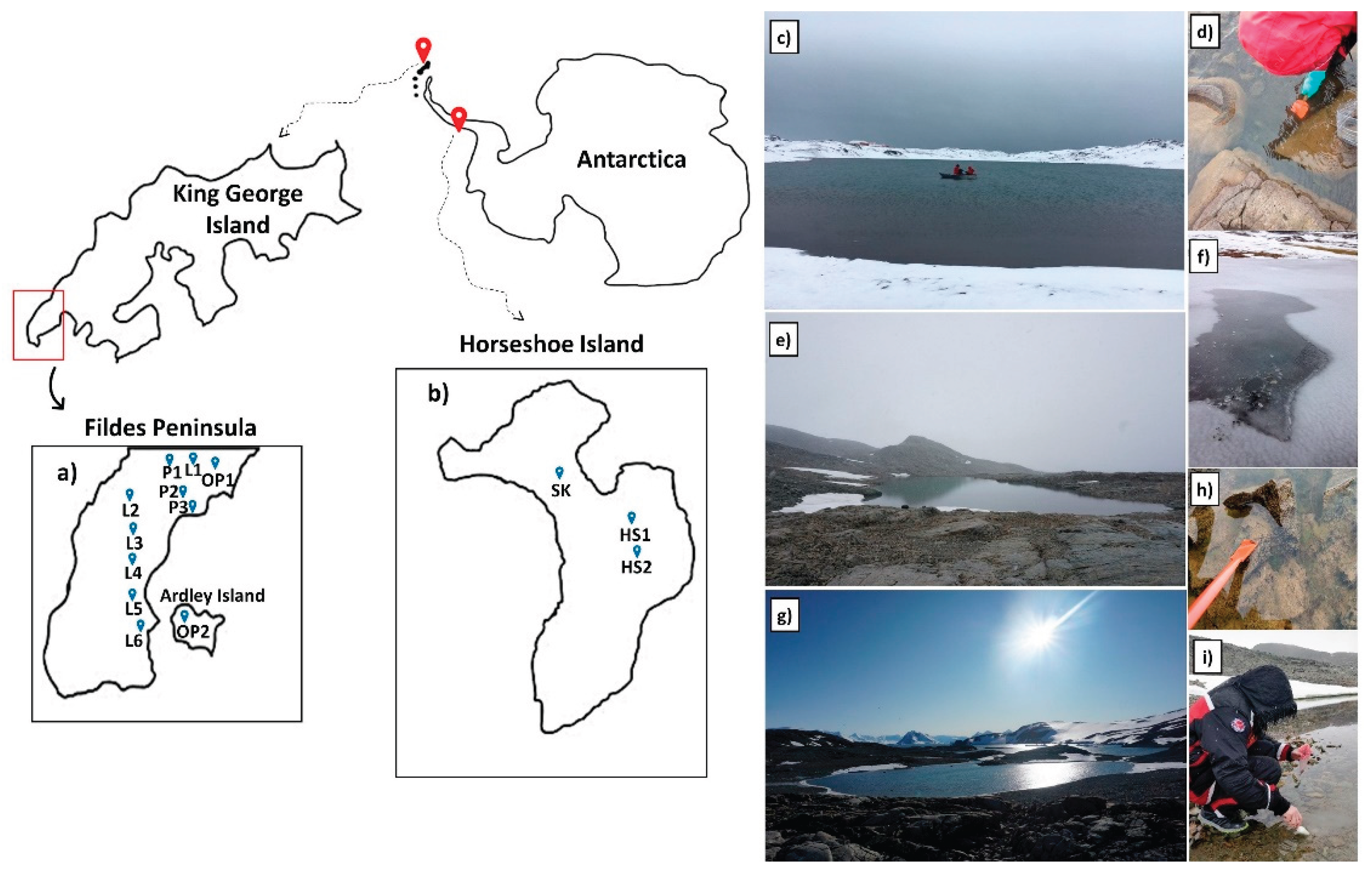
Figure 4.
Correlations between diatom richness and key environmental parameters.
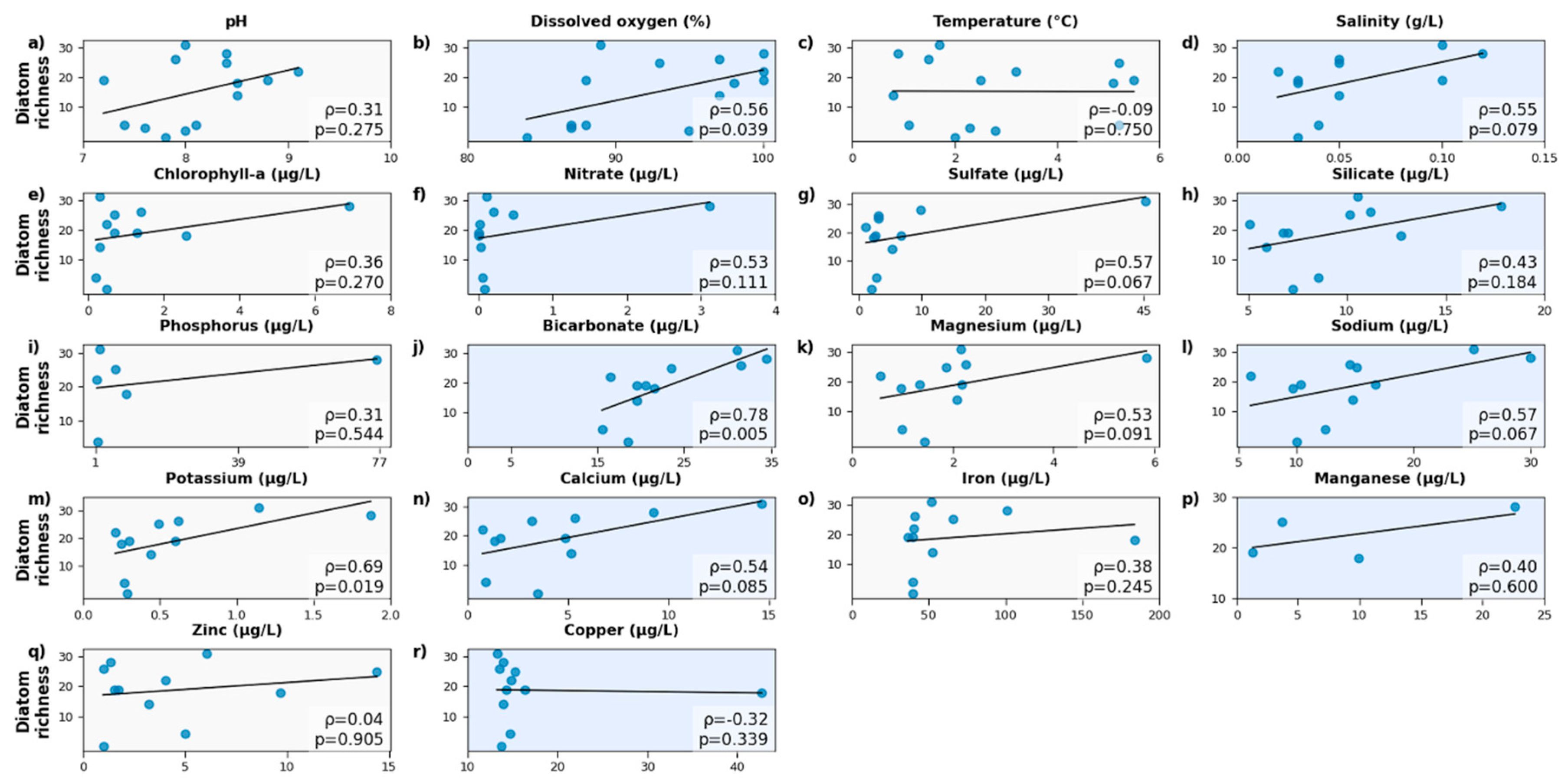

Table 1.
The studied lakes and ponds from King George and Horseshoe Islands with geographic information.
Table 1.
The studied lakes and ponds from King George and Horseshoe Islands with geographic information.
| Sites | Other Name | Abbreviation | Latitude | Longitude | Sampling Date | Sample Type |
|---|---|---|---|---|---|---|
| King George Island - Fildes Peninsula | ||||||
| Lake 1 | Uruguay | L1 | -62.1853 | -58.9118 | 25 Feb 2017 | Water, filter |
| 14 Jan 2019 | ||||||
| Lake 2 | Kitiesh | L2 | -62.1936 | -58.9664 | 19 Feb 2017 | Water, sediment, |
| 17 Jan 2019 | filter | |||||
| Lake 3 | - | L3 | -62.2010 | -58.9729 | 02 Mar 2017 | Water, sediment |
| Lake 4 | Langer | L4 | -62.2050 | -58.9665 | 02 Mar 2017 | Water, sediment |
| 09 Jan 2019 | ||||||
| Lake 5 | West | L5 | -62.2172 | -58.9660 | 02 Mar 2017 | Water, sediment |
| Lake 6 | - | L6 | -62.2210 | -58.9590 | 02 Mar 2017 | Water, sediment |
| Pond 1 | - | P1 | -62.1893 | -58.9295 | 25 Feb 2017 | Water, sediment |
| Pond 2 | - | P2 | -62.1920 | -58.9417 | 25 Feb 2017 | Water, sediment |
| - | -62.2210 | -58.9590 | 09 Jan 2019 | |||
| Pond 3 | - | P3 | -62.1944 | -58.9486 | 25 Feb 2017 | Water, sediment |
| Organic Pond 1 | - | OP1 | -62.1887 | -58.9242 | 25 Feb 2017 | Water, sediment |
| King George Island – Ardley Island | ||||||
| Organic Pond 2 | - | OP2 | -62.2104 | -58.9410 | 02 Mar 2017 | Water, sediment, |
| -62.2104 | -58.9410 | 16 Jan 2019 | filter | |||
| Horseshoe Island | ||||||
| Horseshoe 1 | - | HS1 | -67.22486 | -67.82847 | 21 Feb 2020 | Water, sediment, filter |
| Horseshoe 2 | - | HS2 | -67.22252 | -67.82569 | 21 Feb 2020 | Water, sediment, filter |
| Skua Lake | - | SK | -67.18066 | -67.48444 | 27 Feb 2020 | Water, sediment, filter |
Table 2.
Physicochemical parameters of lakes and ponds in King George and Horseshoe Islands. Water parameters for 2017 sampling were based on [3] and key nutrient, ions and metals concentrations were based on ion chromatography and ICP-MS measurements conducted in [18]. DO: Dissolved Oxygen, Temp.: Temperature, Con.: Conductivity, Salin.: Salinity, TDS: Total Dissolved Solids, Chl-a: Chlorophyll a, ORP: Oxidation Reduction Potential. NA: not available.
| Sites | pH | DO (%) |
Tem. (°C) | Con. (μS cm-1) | Salin. (g/l) | TDS (mg L-1) |
Chl-a (µg L-1) |
ORP (mV) | Key Nutriens (µg/L) | Key Ions (µg/L) | Key Metals (µg/L) | Diatom Species Richness |
|---|---|---|---|---|---|---|---|---|---|---|---|---|
|
L1 (2017) (2019) |
7.4 | 87 | 5.2 | 95 | 0.04 | 48 | 0.2 | NA | NO₃⁻:0.06 PO₄³⁻: <0.001 SO₄²⁻: 2.77 Si: 8.57 P: 1.53 |
HCO₃⁻:15.50 Mg: 1.00 Na: 12.44 K: 0.27 Ca: 0.90 |
Fe: 39.54 Mn: <1 Zn: 5.02 Cu: 14.76 Ni: <1 |
4 |
| 9.2 | 100 | 4.8 | 122 | 0.06 | 61 | NA | 121 | NA | NA | NA | ||
|
L2 (2017) (2019) |
7.2 | 88 | 2.5 | 208 | 0.10 | 104 | 1.3 | NA | NO₃⁻: 0.01 PO₄³⁻: <0.001 SO₄²⁻: 6.61 Si: 6.76 P: <1 |
HCO₃⁻: 20.50 Mg: 2.17 Na: 16.73 K:0.60 Ca: 4.88 |
Fe: 36.20 Mn: <1 Zn: 1.71 Cu: 14.31 Ni: <1 |
19 |
| 11.6 | 101 | 5.1 | 176 | 0.08 | NA | NA | NA | NA | NA | NA | ||
| L3 | 8.5 | 97 | 0.8 | 115 | 0.05 | 58 | 0.3 | NA | NO₃⁻: 0.03 PO₄³⁻: <0.001 SO₄²⁻: 5.27 Si: 5.93 P: <1 |
HCO₃⁻: 19.50 Mg: 2.08 Na:14.78 K: 0.44 Ca: 5.15 |
Fe: 52.50 Mn: <1 Zn: 3.24 Cu: 13.98 Ni: <1 |
14 |
|
L4 (2017) (2019) |
8.0 | 89 | 1.7 | 206 | 0.10 | 103 | 0.3 | NA | NO₃⁻: 0.11 PO₄³⁻: <0.001 SO₄²⁻: 45.35 Si: 10.56 P: 2.21 |
HCO₃⁻: 31.00 Mg: 2.15 Na: 25.12 K: 1.14 Ca: 14.61 |
Fe: 51.62 Mn: <1 Zn: 6.06 Cu: 13.27 Ni: 1.85 |
31 |
| 9.4 | 112 | 8.9 | 313 | 0.15 | 156 | NA | 141 | NA | NA | NA | ||
| L5 | 7.8 | 84 | 2.0 | 75 | 0.03 | 38 | 0.5 | NA | NO₃⁻: 0.08 PO₄³⁻: <0.001 SO₄²⁻: 2.03 Si: 7.25 P: <1 |
HCO₃⁻: 18.50 Mg: 1.43 Na: 9.97 K: 0.29 Ca: 3.47 |
Fe: 39.23 Mn: <1 Zn: 1.02 Cu: 13.72 Ni: <1 |
0 |
| L6 | 7.9 | 97 | 1.5 | 111 | 0.05 | 56 | 1.4 | NA | NO₃⁻: 0.21 PO₄³⁻: <0.001 SO₄²⁻: 3.19 Si: 11.21 P: <1 |
HCO₃⁻: 31.50 Mg: 2.25 Na: 14.55 K: 0.62 Ca: 5.36 |
Fe: 40.82 Mn: <1 Zn: 0.99 Cu: 13.52 Ni: <1 |
26 |
| P1 | 8.8 | 100 | 5.5 | 68 | 0.03 | 34 | 0.7 | NA | NO₃⁻: <0.001 PO₄³⁻: <0.001 SO₄²⁻: 2.58 Si: 7.00 P: <1 |
HCO₃⁻: 19.50 Mg: 1.34 Na: 10.33 K: 0.30 Ca: 1.62 |
Fe: 39.39 Mn: 1.33 Zn: 1.52 Cu: 16.37 Ni: <1 |
19 |
|
P2 (2017) (2019) |
9.1 | 100 | 3.2 | 37 | 0.02 | 18 | 0.5 | NA | NO₃⁻: 0.02 PO₄³⁻: <0.001 SO₄²⁻: 1.16 Si: 5.05 P: 1.38 |
HCO₃⁻: 16.50 Mg: 0.57 Na: 6.04 K: 0.21 Ca: 0.75 |
Fe: 40.22 Mn: <1 Zn: 4.02 Cu: 14.86 Ni: <1 |
22 |
| 9.1 | 99 | 7.1 | 103 | 0.05 | 51 | NA | 145 | NA | NA | NA | ||
| P3 | 8.4 | 93 | 5.2 | 100 | 0.05 | 50 | 0.7 | NA | NO₃⁻: 0.47 PO₄³⁻: <0.001 SO₄²⁻: 3.11 Si: 10.15 P: 6.34 |
HCO₃⁻: 23.50 Mg: 1.86 Na: 15.11 K: 0.49 Ca: 3.22 |
Fe: 65.96 Mn: 3.69 Zn: 14.41 Cu: 15.34 Ni: <1 |
25 |
| OP1 | 8.5 | 98 | 5.1 | 57 | 0.03 | 28 | 2.6 | NA | NO₃⁻: 0.01 PO₄³⁻: <0.001 SO₄²⁻: 2.27 Si: 12.76 P: 9.08 |
HCO₃⁻: 21.50 Mg: 0.97 Na: 9.62 K: 0.25 Ca: 1.36 |
Fe: 183.60 Mn: 9.88 Zn: 9.70 Cu: 42.74 Ni: <1 |
18 |
|
OP2 (2017) (2019) |
8.4 | 100 | 0.9 | 256 | 0.12 | 128 | 6.9 | NA | NO₃⁻: 3.12 PO₄³⁻: <0.001 SO₄²⁻: 9.86 Si: 17.80 P: 76.15 |
HCO₃⁻: 34.50 Mg: 5.84 Na: 29.97 K: 1.87 Ca: 9.25 |
Fe: 100.88 Mn: 22.62 Zn: 1.37 Cu: 13.96 Ni: 1.29 |
28 |
| 9.3 | 108 | 9.2 | 112 | 0.05 | 56 | NA | 103 | NA | NA | NA | ||
| HS1 | 8.0 | 95 | 2.8 | 108 | NA | NA | NA | NA | NA | NA | NA | 2 |
| HS2 | 8.1 | 88 | 1.1 | 122 | NA | NA | NA | NA | NA | NA | NA | 4 |
| SK | 7.6 | 87 | 2.3 | 158 | NA | NA | NA | NA | NA | NA | NA | 3 |
Disclaimer/Publisher’s Note: The statements, opinions and data contained in all publications are solely those of the individual author(s) and contributor(s) and not of MDPI and/or the editor(s). MDPI and/or the editor(s) disclaim responsibility for any injury to people or property resulting from any ideas, methods, instructions or products referred to in the content. |
© 2025 by the authors. Licensee MDPI, Basel, Switzerland. This article is an open access article distributed under the terms and conditions of the Creative Commons Attribution (CC BY) license (http://creativecommons.org/licenses/by/4.0/).
Copyright: This open access article is published under a Creative Commons CC BY 4.0 license, which permit the free download, distribution, and reuse, provided that the author and preprint are cited in any reuse.


