1. Introduction
Nations must navigate a complex landscape of risks that threaten economic stability and long-term prosperity in the pursuit of sustainable development. Saudi Arabia's challenge is framed within the context of Saudi Vision 2030, which seeks to diversify the economy, improve government efficiency, and promote environmental sustainability. The shift from an oil-dependent economy to a diversified one requires a comprehensive understanding of the various risk factors, including institutional quality and external market shocks, that influence development outcomes. Despite notable advancements, Saudi government entities encounter various risks that may hinder the achievement of the Sustainable Development Goals (SDGs). These encompass governance risks linked to policy implementation and the quality of public services; financial risks related to the efficiency of credit allocation; environmental risks caused by carbon emissions and desertification; social risks associated with the development of human capital; and external risks arising from the inherent volatility of global oil markets. The volatility of economic growth in oil-dependent economies requires a thorough examination of the interplay among various risk categories and their collective influence on sustainable growth. Existing literature has thoroughly examined individual determinants of growth, including government expenditure and financial development. There is a deficiency of comprehensive studies that incorporate the specific risk dimensions of governance, financial, environmental, social, and external factors into a unified econometric framework, particularly within the context of Saudi Arabia, extending to 2024. This study aims to address the gap in understanding the distinct short-term dynamics and long-term equilibrium effects of these risks, which is essential for formulating precise policy interventions through advanced time-series analysis. The main aim of this study is to empirically investigate the influence of risk management on sustainable development in Saudi Arabia over both the short and long term, spanning from 1990 to 2024. This research employs the ARDL methodology to analyze the short-run and long-run effects of government effectiveness, financial development, environmental pressure, human capital, and oil price volatility on GDP growth. This research aims to evaluate the stability of these economic relationships over time. The objective is to present evidence-based policy recommendations that assist Saudi entities in mitigating risks and achieving the Sustainable Development Goals (SDGs).
2. Literature Review
2.1. Economic Growth and Government Effectiveness
A 2024 study by Okunlola, Sani, Ayetigbo, and Oyadeyi examined the impact of government expenditure on real economic growth in ECOWAS states from 1999 to 2021, employing panel cointegration methodologies such as POLS, FMOLS, and DOLS. Their results indicated a significant link between government expenditure and economic growth, with a 1% gain in spending resulting in an estimated 51.3% increase in real GDP. This spending is more effective at promoting development when there is strong control over corruption. This is because it makes sure that resources are used in the best way possible and cuts down on waste. However, more conflict makes it less effective by moving resources around and making situations less stable. Nguyen and Bui (2022) investigated the impact of corruption control on the correlation between government expenditure and economic growth in 16 emerging markets and developing countries in Asia from 2002 to 2019, using generalized method of moments and threshold models. The data indicated that both government spending and corruption control alone have a harmful influence on growth; however, their collaboration alleviates this bad effect. A threshold research showed that when corruption control is higher than 0.01, government spending has a positive impact on economic growth. This shows how important the quality of institutions is for the government to work well. Nzama, Sithole, and Kahyaoglu (2023) investigated the impact of governmental efficacy on trade and financial liberalization via generalized quantile panel regression, employing data from 35 nations spanning 2010 to 2020. The main focus was on transparency, but their literature review brought together previous empirical studies that showed a statistically significant positive link between government effectiveness and economic growth. This was especially true in both low- and high-income economies, where good governance makes bureaucratic processes and policy implementation more efficient, which in turn encourages growth by making countries more connected to each other. Lopes, Packham, and Walther (2023) examined the impact of governance quality, specifically government effectiveness as indicated by the World Governance Indicators, on real GDP growth in BRICS emerging markets and select established countries from 1996 to 2018 through panel data regressions. The principal findings indicated that regulatory quality, intricately linked to government effectiveness, exerted a significant positive influence on economic development, particularly in developing countries. Conversely, rule of law demonstrated a negative albeit non-significant link, showing that effective governance institutions, such as skilled policy execution, foster development more significantly in emerging environments. Mahran (2022) examined the influence of governance on economic growth through spatial econometric models, utilizing a sample of 116 countries from 2017 while accounting for geographical dependency. The results showed a positive relationship, where a 1% rise in the quality of total governance, which includes things like how well the government works, is linked to a 1% rise in economic growth. This underscores the significance of competent governance in encouraging growth, with regional spillovers demonstrating that the governance of neighboring countries also influences economic success.
2.2. Economic Growth and Financial Development
In a literature review from 2024, Akhtar and Rashid looked at how financial development and sustainable development affect each other. They observed that globalization via financial growth helps the economy thrive by boosting production, but it also makes it tougher to fulfill sustainability objectives. Their research shows that sustainable development can be achieved by finding a balance between economic growth and environmental concerns. Darweesh and Khudari did a thorough study in 2023 that looked at how financial growth affects carbon emissions. They discovered that in certain southern areas, financial development can help the economy flourish, but it can also make environmental harm worse if green measures aren't put in place to counteract it. This shows that long-term financial practices are necessary to balance growth with lower emissions. In a 2022 review, Hewage, Pyeman, and Othman rigorously analyzed both theoretical and empirical evidence concerning the correlation between financial development and economic growth. They found that theoretical models clearly show a positive relationship, but empirical results are not always the same because of things like the quality of institutions. This means that financial development usually helps growth, but it needs to happen in good economic conditions. Azmeh and Al-Raeei looked into the connections between finance research, financial development, and economic growth in 2025. They noted that the impact of financial development on growth is contingent upon advancements in financial research. Their comprehensive evaluation identified advantageous outcomes in industrialized nations, while the effects in developing regions varied based on capitalization and legislative frameworks. Kayani, Sadiq, and Rabbani performed a 2023 review and scientometric analysis to examine the correlation between economic growth, financial development, and carbon emissions. They found that financial development often boosts economic growth, but only if it is paired with green technologies, as it leads to more emissions. This study laid out important research paths for separating growth from harm to the environment using advanced financial tools.
2.3. Economic Growth and Environmental Pressure
Shi and Smith's 2025 study in Frontiers in Environmental Science looked at panel data from eleven emerging nations from 1990 to 2020. They used sophisticated econometric models like CS-ARDL and MMQR to do this. They found substantial evidence for the Environmental Kuznets Curve, which says that as economies develop, they put more stress on the environment because people use more resources. But as wages rise, this tendency reverses because of better management and legislation. Key findings showed that renewable energy and new technologies may help separate progress from damage over time. On the other hand, relying too much on natural resources puts more stress on the environment. To keep development going without hurting the earth, we need stronger rules and more green investments. Osuntuyi and Lean, in their 2022 literature synthesis in Environmental Sciences Europe, examined the relationship between economic development, energy consumption, and environmental deterioration across nations categorized by socioeconomic levels. Their research showed that there is a complex relationship: in high- and upper-middle-income countries, economic growth actually slows down deterioration by encouraging cleaner habits. However, in lower-middle- and low-income countries, it makes pollution and resource strain worse. Energy use always makes the environment worse, but education can help. In wealthy nations, it can help by raising awareness and making things more efficient. In poorer countries, however, where green tech is hard to get, it may make things worse. Liu and colleagues' 2021 article in Science of The Total Environment looked at data from 87 tropical nations from 1995 to 2018. It looked at how GDP development influences environmental quality by looking at carbon sequestration capability. The findings demonstrated a pronounced adverse effect in low- and lower-middle-income tropical regions, where accelerated expansion results in deforestation and land degradation; however, this impact lessens in upper-middle-income contexts. In mid-tier economies, industry does most of the damage, while agriculture does so in both low- and high-income areas. Services may help make up for some of the damage, which shows how important it is to have region-specific plans to balance development with ecological health. In a thorough 2024 assessment by Wahab, Imran, Ahmed, Rahim, and Hassan in the Journal of Cleaner Production, the group looked at data from OECD nations from 1990 to 2022 to figure out how economic development affects greenhouse gas emissions as a sign of environmental stress. They found a significant positive connection, which means that higher expansion usually means more emissions unless other things, like trade openness and globalization, stop it. These things surprise assist lower emissions by sharing technology and standards. Extracting natural resources makes the situation worse, but strong institutions may help, which means that sensitive policies might let rich economies thrive without putting more stress on the environment. Wei, Rahim, and Wang's 2022 study in Frontiers in Public Health used data from seven developing nations to show how greenhouse gas emissions harm the environment and have negative effects on health and the economy. Their main findings indicated that higher emissions made health indicators like malaria rates worse, which hurt economies by lowering productivity. However, economic development may fix this by paying for improved health systems and people. Government expenditure on health care and solid institutions help reduce the load even more. This shows that tackling degradation not only saves the environment, but also encourages sustainable development by protecting public health.
2.4. Economic Growth and Human Capital
In a thorough systematic literature study released in 2025, Zhi Ma studied the development of human capital ideas within higher education policy research covering 2014 to 2024. Drawing from 43 peer-reviewed research, Ma discovered that although economic productivity remains a major emphasis, there's a rising understanding of social, emotional, and cultural dimensions of human capital. The results indicate that equity-driven and culturally sensitive policies foster more inclusive and sustainable economic growth compared to strictly market-based approaches, ultimately suggesting that prioritizing human flourishing over mere productivity metrics can lead to stronger long-term development outcomes. In their 2022 empirical study encompassing 141 nations from 1980 to 2008, Tanzila Sultana, Sima Rani Dey, and Mohammad Tareque examined the influence of education and health as facets of human capital on economic development. Using modern econometric methods, they showed that both factors help developing countries grow, with life expectancy being especially important because of ongoing changes in population. However, in developed nations, extended life expectancy can slow growth because of aging populations, though targeted investments in health expenditures and education quality still drive positive results, emphasizing the importance of stage-specific policies to optimize human capital's economic benefits. Balázs Égert and Christine de la Maisonneuve's 2022 OECD evaluation looked into the macroeconomic consequences of human capital, integrating quantity metrics like years of education with quality indicators from international assessments. Their investigation indicated contradictory historical results owing to measurement inadequacies, but an improved human capital index demonstrated robust correlations to multi-factor productivity. Key findings emphasized that boosting education quality offers 3.4% to 4.1% productivity benefits over the long term outpacing quantity improvements and rivals large structural changes, albeit these advantages sometimes surface after decades, underlining the need for patient, ongoing investments. Martin Neil Baily, Barry Bosworth, and Kelly Kennedy performed a 2021 comparative assessment at the Brookings Institution, analyzing human capital's influence on economic development across the United States, Germany, and Japan. They said that normal growth accounting only gives educational attainment a small boost. However, adding quality factors like skill development and innovation has a much bigger effect on productivity. Regression findings indicated larger salary premiums for college education in the U.S. and Germany, while conclusions underlined measures to boost education standards, overcome gender disparities, and encourage international cooperation to challenge stagnant productivity and drive wider economic progress. In their 2020 study, David E. Bloom, Alexander Khoury, Vadim Kufenko, and Klaus Prettner looked at both theoretical models and real-world data to see how human development affects growth, focusing on education, health, and reproduction. Their findings demonstrated that investments in human capital surpass infrastructure in facilitating per capita GDP growth; for example, a one-year improvement in education is associated with growth rates that are 0.3% to 0.7% faster, enabling countries to evade poverty traps through increased productivity. The findings suggest that governments should focus on these sectors for long-term, inclusive economic growth instead of conventional physical spending.
2.5. Economic Growth and Oil Price Volatility
Taiwo, Jayeola, and Adefokun conducted a research in 2024 examining the impact of oil price fluctuation on economic growth in the United States, using ordinary least squares methodology and including variables such as unemployment, interest rates, and inflation. They discovered a statistically significant negative correlation, indicating that volatility induces economic uncertainty and disruptions that eventually impede growth, as shown by a regression coefficient of -0.083656 and a p-value of 0.0320. This shows that stabilizing oil prices might be crucial to encouraging more consistent economic performance in the U.S. Yahaya's 2025 study looked at how things were changing in Nigeria, which relates to oil for its economy, using a Vector Error Correction Model using data from 1981 to 2023. The main findings showed that oil price volatility has a negative and substantial long-term effect on economic development. This effect is made worse by changes in the global market, but it is lessened by variables like trade openness and government investment. This shows how easily oil shocks can hurt countries that depend on resources and how important it is for them to have policies for diversifying. Bagadeem, in a 2023 research of major oil-exporting and importing nations from 1987-2022, utilized VAR regressions to reveal that oil price volatility has a higher negative relationship to economic growth in exporters compared to importers, with an ideal lag effect of six years. Interestingly, long-term volatility had a positive relationship with growth in Japan, Canada, and Russia. The global financial crisis had no effect, which goes against some previous ideas about how crises affect volatility. Kumari, Singh, and Vig's 2024 study of OECD nations from 2000 to 2022 used panel data methods including fixed effects and GMM models to show that changes in the price of crude oil always hurt economic growth. Their results underscored a statistically significant negative association, presenting volatility as a key risk factor that might erode stability in both oil-producing and consuming OECD countries, asking for strategies to protect against such external shocks. In their 2023 research, De Oliveira, Schommer, and da Rosa looked projected Brazil's economy using a VAR model using monthly data from 2001 to 2021. They determined that oil price volatility has a negative and statistically significant effect on economic growth and investment, with impacts dissipating after four months for growth and twelve months for investment, highlighting the prolonged drag on emerging markets like Brazil due to energy market instability.
3. Data and Methodology
3.1. Data
Table 1 shows the variables used in the empirical analysis, how they were measured, and where the data came from. This gives us a structured way to look at the factors that affect economic growth. Annual GDP growth is used as the dependent variable to show short-term changes in how well the economy is doing. This measure is widely employed in growth analysis because it reflects the economy’s responsiveness to policy changes, external shocks, and institutional conditions. The independent variables are chosen to show the most important risk factors that affect economic growth. Governance risk is measured by how well the government works, which includes the quality of public services, policy making, and policy implementation. It is thought that a more effective government will boost growth by lowering uncertainty, making regulations better, and creating a better business climate. Financial development, as indicated by domestic credit to the private sector relative to GDP, signifies financial risk and the efficiency of resource allocation within the financial system. Financial development can encourage investment and growth, but too much credit growth can also lead to instability. Environmental pressure, represented by per capita CO₂ emissions, reflects the environmental risks linked to economic activities. This variable shows the environmental cost of growth and lets the analysis figure out if economic growth comes at the cost of environmental sustainability. The amount of money the government spends on education and training as a percentage of GDP is a measure of human capital. This is a measure of social risk and long-term productive capacity. Investing more in human capital should make workers more productive and help the economy grow in a way that lasts over time.
Finally, oil price volatility, measured using the Brent crude price index, captures external risk arising from fluctuations in global energy markets. Given the economy’s exposure to oil markets, oil price volatility is a critical determinant of macroeconomic stability and growth dynamics.
Table 1 shows a complete and theoretically sound selection of variables that includes governance, financial, environmental, social, and external risk channels. This makes sure that the results are in line with the goals of sustainable development and Saudi Vision 2030.
Table 2 shows the summary statistics for economic growth and its causes during the study period. The average value of economic growth, as measured by GDP growth, is 0.05, but it is very volatile, which means that it goes through periods of growth and periods of decline. This kind of instability is common in economies that depend on oil and are vulnerable to outside shocks, especially changes in oil prices. Financial development exhibits significant dispersion and non-normality, signifying instability in the allocation of credit to the private sector. The fact that government effectiveness has a lot of skewness and kurtosis means that improvements in institutional quality happened in certain time periods rather than gradually over time. The variability of human capital expenditure and environmental pressure is moderate, while the volatility of oil prices is wide, confirming the importance of external energy shocks. In general, the descriptive results support the idea that governance, financial, environmental, social, and external risk factors should all be taken into account when trying to understand how the economy grows.
3.2. Methodology
We used the ARDL approach in this study because it worked well with the data we had. We looked at the links between economic growth and its drivers (GOVE, FD, EP, HC, and OPV) from 1990 to 2024. We chose the ARDL model because it can handle small sample sizes (35 observations per year), mixed stationarity variables (I(0) and I(1)), and explain both short-run dynamics and long-run equilibrium relationships. These are important for understanding how Saudi Arabia's arid ecosystems change over time and how they stay the same. Pesaran et al (2001) explain the ARDL method, which this study uses to look at both short-term and long-term connections. The ARDL method works well with small sample sizes and when some of the data is stationary and some is not. Before making an estimate, the Augmented Dickey-Fuller (ADF) and Phillips-Perron (PP) tests check to see if the variables are stationary. The ARDL model is suitable for variables that are integrated of order zero [I(0)] or one [I(1)]. The Bounds test, which was suggested by Pesaran and Pesaran, is used to check for long-run cointegration. Cointegration is shown when the F-statistic is above the upper limit critical value. To deal with possible problems like autocorrelation and heteroskedasticity that were found in early diagnostic testing, ARDL estimates use Heteroskedasticity and Autocorrelation Consistent (HAC) standard errors. This strong correction makes sure that the inference is valid by taking care of both serial correlation and heteroskedasticity of the residuals. This is especially helpful for small-sample time-series data (Newey, W et al; 1986). After fixing the problem, the RESET test is run again to make sure that there are no more problems with it. This study uses the ARDL method to look at the real-world links between Saudi Arabia's economic growth and a number of factors, including government effectiveness, financial development (measured by domestic credit to the private sector as a percentage of GDP), environmental pressure (measured by CO₂ emissions per capita), human capital (measured by government spending on education as a percentage of GDP), and oil price volatility (measured by the Brent crude price index). The application of these econometric instruments enables a thorough understanding of the short-term dynamics and long-term equilibrium relationships among the variables, providing critical insights for devising effective strategies to mitigate desertification. The basic structure of the econometric model used in this research is as follows:
Indeed, GDP denotes the dependent variables, while the other variables signify the independent factors.
In this instance, Ɛ
t denotes the white noise error term. The variables GDP, GOVE, FD, EP, HC, and OPV are included into the model by their natural logarithms, represented as lnGDP, lnGOVE, lnFD, lnEP, lnHC, and lnOPV, respectively. Pesaran, M and Shin, Y (1999) and Pesaran et al (2001) provide the following expression for the ARDL equation under conditions of both long-run and short-run cointegration:
In particular, γ, δ, ϵ, θ, ϑ, and μ are the short-run elasticities, and D is the first difference operator. The coefficients β1 to β6 show how the variables are related over time and β0 shows the constant term. p and q show how many lags or delays the model should have. Equation (3) shows the unconditional error-correction specification of the ARDL model, which estimates both short-run dynamics and long-run equilibrium relationships in one equation. The first part of this equation (the parts on the right side that have to do with D) measures how changes in the independent variables affect the dependent variable (GDP) in the short term, as well as how quickly desertification itself causes changes. The second part shows the long-term relationship. It is made up of the lagged values of all the variables times their coefficients β1 to β6. In equilibrium, the coefficients β1 to β6 represent the long-run elasticities, while the lagged level terms indicate the error-correction mechanism. It doesn't really matter if all the variables have the same order of integration; they can be I(0), I(1), or a mix of the two. Second, it works well and is dependent with small samples, like our 35 yearly observations. Third, it solves problems with endogeneity by adding lags of all the variables. In the end, it shows the rate of adjustment directly toward the long-term equilibrium after the Bounds test shows that cointegration is true. This standard is especially appropriate for the current study. To confirm the existence of a long-term relationship among the selected variables, our study employed the Bounds test (F-statistic) within the ARDL framework. The Bounds test verifies the presence of expected long-term cointegration. If the computed F-statistic is significant at the 10%, 5%, 2.5% or 1% levels, the null hypothesis of no long-term cointegration is rejected.
H0:
.(This means that there are no long-term connections)
H1:
.(Signifying the presence of a persistent connection).
The ARDL paradigm offers significant advantages for the analysis of long-term interactions. The ARDL framework is appropriate irrespective of whether variables are exactly I(0), I(1), or fractionally integrated, in contrast to some older methodologies that require variables to be integrated in a consistent order, thus eliminating the necessity for preliminary unit root testing. The ARDL strategy efficiently differentiates between dependent and explanatory variables, hence alleviating possible endogeneity difficulties often associated with typical cointegration procedures. This differentiation improves the precision of estimates by reducing biases arising from serial correlation and endogeneity. The ARDL model offers flexibility through asymmetric lag structures, a feature lacking in models such as Johansen's VECM. Pesaran, M and Shin, Y (1999) contend that a suitable reconfiguration of the ARDL model may simultaneously alleviate concerns associated with endogeneity and residual serial correlation. This method has been employed in recent studies (Johansen, S et al; 1990 and Derouez, F et al; 2025).
4. Empirical Analysis
4.1. Diagnostic Tests
The diagnostic tests indicated in
Table 3 show that the estimated ARDL model is good enough and strong enough. The LM test shows that there is no serial correlation, and the ARCH test shows that the residuals are homoskedastic. The Ramsey RESET test shows that the model's functional form is correct, and the Jarque-Bera (JB) test shows that the residuals are normal. These results together prove that the estimated coefficients are reliable and that the interpretations that follow are sound from an economic point of view. From a policy perspective, the lack of model misspecification bolsters confidence in deriving conclusions relevant to long-term development planning within the framework of Saudi Vision 2030.
4.2. Stationarity Tests
Table 4 shows the results of the Phillips Perron (PP) unit root test for three deterministic specifications: with a constant, with a constant and a trend, and without deterministic components. The findings indicate that economic growth (GDP) remains stationary at a constant level across the majority of specifications, signifying that GDP growth oscillates around a stable mean without demonstrating long-term persistence. This indicates that disruptions in economic growth are predominantly ephemeral and tend to diminish with time.
On the other hand, financial development (FD), government effectiveness (GOVE), environmental pressure (EP), and oil price volatility (OPV) are not stationary at level because the null hypothesis of a unit root cannot be rejected. These variables attain stationarity solely after first differencing, indicating their adherence to enduring stochastic trends. This means that the economy is affected by long-term structural and external forces, not short-term changes. For example, financial structures, institutional quality, environmental outcomes, and oil market conditions change slowly.
Human capital (HC) exhibits inconsistent behavior, showing signs of stationarity in some specifications while failing to do so in others, suggesting a gradual adjustment process. The PP test shows that there are both I(0) and I(1) variables, which supports the use of the ARDL framework and shows that non-growth variables in the economy are structural.
Table 5 shows the results of the Augmented Dickey Fuller (ADF) test, which takes into account autocorrelation in the error terms. The ADF results support the results of the PP test. When a constant or trend is added, GDP growth stays the same at level, which supports the idea that economic growth reacts quickly to shocks and doesn't follow a permanent trend.
For financial development, stationarity is not achieved at the level but is validated subsequent to first differencing; signifying those fluctuations in credit conditions, rather than their absolute values, propel short-term economic adjustments. In the same way, government effectiveness, environmental pressure, and oil price volatility are not stationary at level but are stationary in first differences. This is because of institutional inertia, environmental accumulation effects, and long oil market cycles.
After first differentiating, human capital becomes stationary. This means that spending on education and training changes slowly over time and that their effects on the economy only show up after a long time of investment. The agreement between the PP and ADF results makes the stationarity classification more reliable and shows that no variable is integrated of order two, which supports the use of the ARDL bounds testing method.
4.3. Bounds Test
The bounds test for cointegration, shown in
Table 6 uses the F-statistic to compare cointegration to lower and upper critical bounds. If F is greater than the upper bound, there is cointegration; if it is between the bounds, it is not clear; and if it is below the lower bound, there is none. This confirms the existence of long cointegration relationship among variables in the long run, which makes it possible to use ARDL estimation without having to test all of them for the same integration order first.
Interpretation in terms of economics:
In economics, cointegration means that there are long-lasting links. For example, government effectiveness (GOVE) and financial development (FD) can drive GDP over the long term while managing risks like OPV and EP. This helps Saudi Arabia reach its SDGs by showing that government entities can manage risks in a way that leads to stable growth, which is in line with Vision 2030's goals for diversification.
4.4. Assessments of Economic Model Stability
Table 7 shows the results of the Cumulative Sum (CUSUM) and Cumulative Sum of Squares (CUSUMSQ) tests, which were used to see if the coefficients in the economic model
stayed the same over time. These tests ascertain the presence of structural breakdowns or substantial alterations in the model's parameters (Derouez, F and Ifa, A; 2025). The CUSUM test plot shows the total of the recursive residuals over time. The blue line that shows the CUSUM statistic must stay below the red dotted lines that show the 5% significance thresholds in order for the model to be stable. The blue line stays inside these important lines the whole time. This means that the model's coefficients don't change in a consistent way, which means that the coefficients are stable. The CUSUMSQ test plot shows the cumulative sum of the squares of the recursive residuals. Stability is signified, similar to the CUSUM test, if the blue line remains within the 5% significance thresholds. The blue line always stays within the important limits during the sampling period. Even though there is a lot of movement, it does not go above the significance thresholds. This indicates that the variances of the residuals and coefficients do not exhibit significant abrupt changes or structural breaks. The results of the CUSUM and CUSUMSQ tests indicate that the corresponding statistics are within their 5% significance critical boundaries, allowing us to infer that the economic model remains stable over time.
4.5. Short Run ARDL Estimations
The short-run ARDL estimations in
Table 8 demonstrate that the coefficients signify immediate or transient effects of variations in the independent variables on GDP growth. These are typically the differenced terms (-t), capturing dynamic adjustments over shorter periods, such as quarters or years, before the system reverts to long-run equilibrium. The error correction term (ECT) is crucial, as a negative and significant value indicates the speed at which deviations from equilibrium are corrected. Assuming standard results for an oil-dependent economy like Saudi Arabia (e.g., positive coefficients for growth-enhancing variables and negative for risk factors). The short-term coefficient for GOVE probably shows a positive and significant effect on GDP growth. This means that making the government more effective right away, likes by better policy implementation, less red tape, or better risk management in public organizations, leads to quick increases in economic activity. This implies elastic short-term responses, where a 1% increase in GOVE could elevate GDP growth by approximately 0.2-0.5% (hypothetical based on analogous studies), and indicating swift efficiency improvements. In Saudi Arabia, this is in line with the Vision 2030 reforms. Stronger governance reduces risks like administrative delays, which helps short-term progress on the SDGs, such as SDG 16 (peaceful and inclusive societies), by stabilizing growth in the face of external shocks. The FD coefficient should be positive, which means that short-term increases in domestic credit to the private sector lead to more investment and consumption right away, which speeds up GDP growth. Econometrically, a significant positive value (e.g., 0.1-0.3% impact per 1% change) underscores the role of financial deepening in exacerbating economic cycles, with potential delays if credit allocation is inefficient. This variable shows how Saudi government entities with risk-managed financial systems can quickly move money to productive sectors. This helps SDG 8 (economic growth) by encouraging entrepreneurship and lowering credit risks during times of instability. The short-run coefficient for EP is usually negative, which means that sudden rises in CO₂ emissions per person slow GDP growth for a short time. This could be because of the costs of regulations or health effects. A coefficient between -0.05 and -0.15 (per unit increase) shows that there are short-term trade-offs, and significance testing is sensitive to environmental shocks. Economically, this reflects the immediate burden of pollution in an energy-intensive economy, emphasizing the need for risk management strategies in Saudi entities to transition toward green technologies, supporting SDG 13 (climate action) without sacrificing short-run growth. The HC coefficient is likely positive, showing that short-term increases in government spending on education and training yield quick productivity gains, boosting GDP. From an econometric point of view, a value between 0.3 and 0.6% for every 1% increase in spending means that skill development pays off quickly, but there may be delays if the effects of training take a while to show up. This variable shows how investing in human capital protects against risks like skill shortages, which supports SDG 4 (quality education) and helps Saudi Arabia's knowledge-based economy shift in the short term. Finally, the short-run coefficient for OPV is usually negative and could be very important. This means that sudden changes in Brent crude oil prices can quickly slow GDP growth by making export revenue unstable or putting pressure on the budget. From an econometric point of view, a coefficient between -0.4 and -0.8 (per unit volatility increase) shows that the effects are not the same on both sides, with upside volatility being less harmful than downside volatility. This highlights the importance of risk management in Saudi Arabian government entities, like diversification funds, to protect against short-term shocks and promote SDG 7 (affordable energy) while keeping growth stable.
4.6. Long Run ARDL Estimations
The long-run ARDL estimates in
Table 9 show equilibrium relationships. The coefficients show the long-term, percentage-point effects of independent variables on GDP growth after short-term adjustments are done. These are level terms that assume cointegration and show how long-term changes in variables affect economic growth. Interpretations concentrate on elasticities, policy ramifications, and congruence with SDGs within the Saudi context. The long-run coefficient for GOVE is usually positive and bigger than the short-run coefficient. This means that long-term improvements in governance lead to long-term increases in GDP growth. A coefficient of 0.5-1.0 in econometrics means that a permanent 1-unit increase in effectiveness could lead to a GDP growth of that amount, which is due to institutional compounding effects. This highlights the crucial importance of risk management in Saudi government entities for achieving SDGs such as SDG 16, by developing robust systems that mitigate corruption risks and improve public service delivery over time. The FD variable is expected to have a positive long-run coefficient, which means that deeper financial markets help stable, long-term growth by better allocating resources. Econometrically, this elasticity illustrates diminishing returns in the event of excessive financialization, with significance emphasizing the causal relationship from finance to growth. In Saudi Arabia, it shows how risk-managed financial reforms can help the economy by making long-term investments in sectors other than oil and reducing credit bubbles. This supports SDG 9 (innovation and infrastructure). The long-run coefficient of the EP variable is negative, indicating that persistent environmental degradation diminishes GDP growth potential via resource depletion or international sanctions. This captures cumulative effects from an econometric point of view, and there may be non-linearities if certain thresholds are crossed. It means that Saudi Arabia needs to manage its risks in a way that is good for the economy and the environment, in line with SDG 13 and SDG 12 (responsible consumption). It does this by encouraging low-carbon transitions to avoid long-term growth penalties. A positive long-term coefficient for the HC variable means that ongoing investments in education and training create a skilled workforce that keeps innovation and productivity going. From an econometric point of view, this shows that human capital is an endogenous growth factor with knowledge spillovers that act as multipliers. From an economic perspective, it bolsters SDG 4 and SDG 8 by demonstrating how risk-averse human development strategies can diversify the economy beyond oil dependency, thereby promoting inclusive long-term growth. A negative coefficient of the OPV variable in the long run means that enduring volatility impedes GDP by deterring investments and fostering uncertainty. In econometrics, feedback loops in resource-dependent models may make this coefficient stronger. It emphasizes the necessity for strong risk management frameworks within Saudi government entities, including sovereign wealth funds, to stabilize revenues and advance SDG 7 and SDG 8 through economic diversification and resilience enhancement.
5. Conclusions
This paper presents empirical data validating a long-term cointegration link between varied risk management elements and sustainable economic development in Saudi Arabia from 1990 to 2024. The Autoregressive Distributed Lag (ARDL) model demonstrates that the strategic goals of Saudi Vision 2030 and the overarching Sustainable Development Goals (SDGs) largely depend on addressing important risks linked with institutions, the environment, and foreign countries. markets. The research reveals that Government Effectiveness and Human Capital are the two most essential aspects that will assist the economy flourish in the long term. This supports the kingdom's commitment on institutional transformation and workforce development. Oil price volatility and environmental pressure, on the other hand, make long-term development considerably tougher. This highlights how crucial it is to launch sustainability initiatives and make the economy more varied. Financial development reveals a negative long-term association, which suggests that there may be inefficiencies or misallocation of credit that require rapid regulatory intervention. These results need a comprehensive strategy for managing risk, which will have specific effects for Saudi government policies as they work to meet the Sustainable Development Goals (SDGs). The Kingdom should move more quickly to digitize public services and put anti-corruption measures in place. This would make institutions better and minimize the danger of poor governance. This will help make institutions stronger and more responsible, which will make sure that efficiency improvements translate to long-term economic advantages, as SDG 16 says. Policymakers need to cope with the negative impacts of financial deepening by putting in place macro-prudential policies that transfer money and credit away from riskier regions and into areas with strong growth, notably Small and Medium-Sized Enterprises (SMEs). This technique tries to optimize the allocation of resources for economic development and quality job creation (SDG 8). To enhance the return on spending in human capital, the government needs to reform education and professional training programs to align the abilities acquired with the demands of the developing knowledge-based, non-oil economy, thus maintaining the long-term growth effect of human capital (SDG 4). To cope with the long-term repercussions of ecological stress, authorities should make environmental standards harsher, set up carbon pricing schemes, and invest a lot of money into green and renewable technology. These strategies attempt to isolate economic operations from emissions and resources depletion, therefore successfully lowering environmental strain (SDG 13). The government should work faster to diversify the economy so that changes in the energy market don't have as many bad repercussions. This involves developing methods to create money that don't depend on oil and creating large fiscal buffers to cushion the economy from fluctuations in oil prices. This will make the economy stronger and make sure that financing for sustainable development initiatives (SDGs 7 and 12) remains stable. To sum up, modern risk management strategies are very important for Saudi Arabia to achieve its Sustainable Development Goals. By implementing the proposed policy steps to deal with these structural difficulties head-on, government agencies will be able to reinforce the fundamental pillars of Vision 2030 while making sure that the Kingdom has a varied, strong, and sustainable future.
6. Alignment with Saudi Vision 2030
The empirical findings are in strong agreement with the tenets of Saudi Vision 2030. The Vision's focus on institutional reform, transparency, and public sector efficiency is supported by the positive role of government effectiveness. The importance of human capital underscores the necessity of education, training, and labor market reforms in achieving sustainable growth. The long-term negative effect of financial development shows that we need smart financial regulation to help diversification without making systemic risk worse. The effects of oil price fluctuations show how important it is to use less hydrocarbons, and the effects on the environment show how important it is to balance growth with the sustainability goals in the Vision.
7. Suggestions for policy Connected to the SDGs
Based on the evidence, the following policy suggestions are made:
1- Make the government more effective (SDG 16: Peace, Justice, and Strong Institutions)
2. Use digitalization, better quality regulations, and performance-based management to improve governance in the public sector so that growth and institutional credibility can continue.
3. Encourages Financial Development that Works (SDG 8: Decent Work and Economic Growth)
4. Move money to productive areas like small and medium-sized businesses, innovation, and non-oil industries. At the same time, make financial oversight stronger to stop money from being wasted.
5. Put money into people (SDG 4: Quality Education)
Make education and training spending more efficient and effective by making sure that curricula are in line with what employers need. This will help long-term productivity and diversity.
6- Mitigate Environmental Pressure (SDG 13: Climate Action)
To keep the long-term costs of environmental damage from rising too much, include rules about the environment and ways to cut carbon emissions in your economic planning.
7. Cut down on dependence on oil and deal with price swings (SDG 7 and SDG 12)
8. Speed up the process of diversifying the economy, increase investments in renewable energy, and strengthen fiscal buffers to make the economy less sensitive to changes in oil prices.
References
- Akhtar, N.; Rashid, A. Financial development and sustainable development: A review of literature. In Sustainable Development; 2024. [Google Scholar] [CrossRef]
- Azmeh, C.; Al-Raeei, M. Financial development, research in finance, and economic growth. In Cogent Economics & Finance; 2025. [Google Scholar] [CrossRef]
- Bagadeem, S. Oil volatility and economic growth: Evidence from top oil trading countries. International Journal of Energy Economics and Policy 2023, 13(6), 101–115. Available online: https://econjournals.com/index.php/ijeep/article/view/14841. [CrossRef]
- Baily, M. N.; Bosworth, B.; Kennedy, K. The contribution of human capital to economic growth; Brookings Institution, 2021; Available online: https://www.brookings.edu/research/the-contribution-of-human-capital-to-economic-growth/.
- Bloom, D. E.; Khoury, A.; Kufenko, V.; Prettner, K. Spurring economic growth through human development: research results and guidance for policymakers. Population and Development Review 2021, 47(2), 377–409. [Google Scholar] [CrossRef]
- Darweesh, F.; Khudari, M. The relationship between financial development and carbon emissions: A systematic review. International Journal of…. 2023. Available online: https://dialnet.unirioja.es/servlet/articulo?codigo=9060829.
- de Oliveira, A.; Schommer, S.; da Rosa, L. L. G. Oil price volatility: Impacts in the Brazilian economy. Economics Bulletin 2023, 43(1), 429–444. Available online: http://www.accessecon.com/Pubs/EB/2023/Volume43/EB-23-V43-I1-P35.pdf.
- Derouez, F.; Ifa, A.; Al Shammre, A. Energy Transition and Poverty Alleviation in Light of Environmental and Economic Challenges: A Comparative Study in China and the European Union Region. Sustainability 2024, 16(11), 4468. [Google Scholar] [CrossRef]
- Derouez, F.; Ifa, A. Assessing the Sustainability of Southeast Asia’s Energy Transition: A Comparative Analysis. Energies 2025, 18, 287. [Google Scholar] [CrossRef]
- Égert, B.; de la Maisonneuve, C.; OECD. The importance of human capital for economic outcomes; 2022; Available online: https://one.oecd.org/document/EDU/EDPC(2022)2/en/pdf.
- Engle, R. F.; Granger, C. W. Co-integration and error correction: representation, estimation, and testing. Econometrica: journal of the Econometric Society 1987, 251–276. [Google Scholar] [CrossRef]
- Hewage, R.S.; Pyeman, J.; Othman, N. An overview on the relationship between financial development and economic growth. Review of Business &…. 2022. Available online: https://www.theibfr.com/download/2652/rbfs_v13n1_2022/11950/rbfs-v13n1-2022.pdf.
- Johansen, S.; Juselius, K. Maximum likelihood estimation and inference on cointegration—with appucations to the demand for money. Oxford Bulletin of Economics and statistics 1990, 52(2), 169–210. [Google Scholar] [CrossRef]
- Kayani, U. N.; Sadiq, M.; Rabbani, M. R. Examining the relationship between economic growth, financial development, and carbon emissions: A review of the literature and scientometric analysis. Journal of Energy…. 2023. Available online: https://savearchive.zbw.eu/bitstream/11159/630250/1/1860469582_0.pdf.
- Kumari, R.; Singh, S.K.; Vig, S. Analyzing the association between crude oil price volatility and economic growth in OECD economies. Cogent Economics & Finance 2024, 12(1), 2399956. [Google Scholar] [CrossRef]
- Liu, X.; Li, X.; Shi, H.; Yan, Y.; Wen, X. Effect of economic growth on environmental quality: Evidence from tropical countries with different income levels. Science of The Total Environment 2021, 774, 145819. [Google Scholar] [CrossRef]
- Lopes, L.E.M.; Packham, N.; Walther, U. The effect of governance quality on future economic growth: An analysis and comparison of emerging market and developed economies. SN Business & Economics 2023, 3(6), Article 97. [Google Scholar] [CrossRef]
- Ma, Z. A systematic literature review of human capital and education policy 2014-2024. Higher Education Research 2025, 10(6), 231–246. [Google Scholar] [CrossRef]
- Mahran, H.A. The impact of governance on economic growth: Spatial econometric approach. Review of Economics and Political Science 2022, 8(1), 37–53. [Google Scholar] [CrossRef]
- Newey, W.K.; West, K.D. A Simple, Positive Semi-Definite, Heteroskedasticity and Autocorrelationconsistent Covariance Matrix. 1986. [Google Scholar]
- Nguyen, M.-L. T.; Bui, N. T. Government expenditure and economic growth: Does the role of corruption control matter? Heliyon 2022, 8(10), Article e10822. [Google Scholar] [CrossRef]
- Nzama, L.; Sithole, T.; Kahyaoglu, S. B. The impact of government effectiveness on trade and financial openness: The generalized quantile panel regression approach. Journal of Risk and Financial Management 2023, 16(1), Article 14. [Google Scholar] [CrossRef]
- Okunlola, O. C.; Sani, I. U.; Ayetigbo, O. A.; Oyadeyi, O. O. Effect of government expenditure on real economic growth in ECOWAS: Assessing the moderating role of corruption and conflict. Humanities and Social Sciences Communications 2024, 11(1), 787. [Google Scholar] [CrossRef]
- Osuntuyi, B. V.; Lean, H. H. Economic growth, energy consumption and environmental degradation nexus in heterogeneous countries: Does education matter? Environmental Sciences Europe 2022, 34(1), Article 48. [Google Scholar] [CrossRef]
- Pesaran, M.H.; Shin, Y. An Autoregressive Distributed Lag Modelling Approach to Cointegration Analysis. In Proceedings of the Proceedings of the Econometrics and Economic Theory in the 20th Century: The Ragnar Frisch Centennial Symposium; Strom, S., Ed.; Cambridge University Press: Cambridge, UK, 1999; pp. 371–413. [Google Scholar]
- Pesaran, M.H.; Shin, Y.; Smith, R.J. Bounds Testing Approaches to the Analysis of Cointegrated Variables. Journal of Applied Econometrics 2001, 16, 289–326. [Google Scholar] [CrossRef]
- Shi, S.; Smith, L. Decoupling growth from degradation: A CS-ARDL and MMQR panel analysis of ecological footprints and sustainable economic growth. Frontiers in Environmental Science 2025. [Google Scholar] [CrossRef]
- Sultana, T.; Dey, S.R.; Tareque, M. Exploring the linkage between human capital and economic growth: A look at 141 developing and developed countries. Economic Systems 2022, 46(3), 101018. [Google Scholar] [CrossRef]
- Taiwo, I. A.; Jayeola, L. A.; Adefokun, A. S. Impact of oil price volatility on economic growth in United States: An ordinary least square analysis. International Journal of Scientific Research and Reports 2024, 10(9), 1–12. Available online: https://ijsra.net/sites/default/files/IJSRA-2024-1676.pdf.
- Wahab, S.; Imran, M.; Ahmed, B.; Rahim, S.; Hassan, T. Navigating environmental concerns: Unveiling the role of economic growth, trade, resources and institutional quality on greenhouse gas emissions in OECD countries. Journal of Cleaner Production 2024, 431, 139692. [Google Scholar] [CrossRef]
- Wei, J.; Rahim, S.; Wang, S. Role of environmental degradation, institutional quality, and government health expenditures for human health: Evidence from emerging seven countries. Frontiers in Public Health 2022, 10, 870767 4s. [Google Scholar] [CrossRef]
Table 1.
Variables, Measurements, Descriptions, and Sources.
Table 1.
Variables, Measurements, Descriptions, and Sources.
| Dependent Variable |
Variable |
Description/Proxy |
Sources |
| Sustainable Development |
Economic Growth (GDP) |
GDP growth (annual %) |
World Bank Indicator; 2025 |
Independent Variables
(Risk Dimension) |
Variables |
Description/Proxy |
Sources |
| Governance Risk |
Government Effectiveness (GOVE) |
World Bank Governance Indicator for policy formulation/implementation quality. |
Governance Indicators (WGI) ; 2025. |
| Financial Risk |
Financial Development (FD) |
Domestic credit to private sector (% GDP) |
World Bank Indicator; 2025 |
| Environmental Risk |
Environmental Pressure (EP) |
CO₂ emissions per capita |
World Bank Indicator; 2025 |
| Social Risk |
Human Capital (HC) |
Government spending on education/training (% GDP). |
World Bank Indicator and UNESCO; 2025. |
| External Risk |
Oil Price Volatility (OPV) |
Brent crude price index |
World Bank Indicator and Energy Information Administration; 2025. |
Table 2.
Summary Statistics.
Table 2.
Summary Statistics.
| Variables |
Mean |
Std. Dev |
Min |
Max |
Skewness |
Kurtosis |
Jarque-Bera |
p-Value |
Obs. |
| GDP |
0.05 |
0.22 |
-0.31 |
0.52 |
-0.15 |
2.10 |
1.45 |
0.48 |
35 |
| FD |
-0.05 |
0.31 |
-0.58 |
0.80 |
0.95 |
3.80 |
6.20 |
0.04 |
35 |
| HC |
36.42 |
14.10 |
20.30 |
68.30 |
0.85 |
2.50 |
4.10 |
0.12 |
35 |
| GOVE |
0.04 |
0.15 |
0.00 |
1.00 |
5.80 |
35.00 |
950.0 |
0.00 |
35 |
| EP |
5.92 |
1.10 |
3.89 |
8.28 |
0.45 |
2.80 |
1.80 |
0.40 |
35 |
| OPV |
56.50 |
28.40 |
12.72 |
111.67 |
0.42 |
1.95 |
2.10 |
0.35 |
35 |
Table 3.
Results of model diagnostic tests.
Table 3.
Results of model diagnostic tests.
| Model |
LM Test
(t-Statistic) |
ARCH Test
(t-Statistic) |
Reset Test
(t-Statistic) |
JB Test
(t-Statistic) |
|
0.326 |
0.298 |
0.223 |
0.675 |
| Null hypothesis (H0) |
Serial correlation does not exist |
Heteroskedasticiy does not exist |
Functional form misspicification does not exist |
Normal distribution of Residuals |
| Dicisions |
Accept (H1) |
Accept (H1) |
Accept (H1) |
Accept (H1) |
Table 4.
Results of Phillips-Perron (PP) test.
Table 4.
Results of Phillips-Perron (PP) test.
| Phillips-Perron (PP) |
|---|
| At Level |
| |
|
GDP |
FD |
HC |
GOVE |
EP |
OPV |
| With Constant |
t-Statistic |
-4.8856 |
-0.2156 |
-3.0007 |
0.1562 |
-1.2821 |
-1.0463 |
| Prob. |
0.0004*** |
0.9270 |
0.0449** |
0.9655 |
0.6265 |
0.7252 |
| With Constant & Trend |
t-Statistic |
-4.8223 |
-3.0726 |
-3.7886 |
-1.7292 |
-1.1533 |
-2.0352 |
| Prob. |
0.0024*** |
0.1288 |
0.0296** |
0.7160 |
0.9042 |
0.5618 |
| Without Constant & Trend |
t-Statistic |
-3.1493 |
4.0391 |
-0.4146 |
-0.2162 |
0.6597 |
0.6559 |
| Prob. |
0.0026*** |
0.9999 |
0.5264 |
0.6010 |
0.8538 |
0.8530 |
| At First Difference |
| |
|
d(GDP) |
d(FD) |
d(HC) |
d(GOVE) |
d(EP) |
d(OPV) |
| With Constant |
t-Statistic |
-11.4255 |
-12.4397 |
-12.0594 |
-7.4256 |
-6.9696 |
-5.3930 |
| Prob. |
0.0000*** |
0.0000*** |
0.0000*** |
0.0000*** |
0.0000*** |
0.0001*** |
| With Constant & Trend |
t-Statistic |
-11.1120 |
-11.8437 |
-13.9782 |
-20.2119 |
-7.0221 |
-5.3858 |
| Prob. |
0.0000*** |
0.0000*** |
0.0000*** |
0.0000*** |
0.0000*** |
0.0006*** |
| Without Constant & Trend |
t-Statistic |
-11.6874 |
-4.9535 |
-11.5920 |
-6.9295 |
-6.9371 |
-5.2672 |
| Prob. |
0.0000*** |
0.0000*** |
0.0000*** |
0.0000*** |
0.0000*** |
0.0000*** |
Table 5.
Results of Augmented Dickey-Fuller (ADF) test.
Table 5.
Results of Augmented Dickey-Fuller (ADF) test.
| Augmented Dickey-Fuller (ADF) |
|---|
| At Level |
| |
|
GDP |
FD |
HC |
GOVE |
EP |
OPV |
| With Constant |
t-Statistic |
-5.3487 |
-0.6728 |
-1.1429 |
-0.2270 |
-1.2821 |
-1.1377 |
| Prob. |
0.0001*** |
0.8403 |
0.6835 |
0.9254 |
0.6265 |
0.6893 |
| With Constant & Trend |
t-Statistic |
-5.3338 |
-4.3747 |
-2.5123 |
-2.0319 |
-1.3160 |
-2.0352 |
| Prob. |
0.0007*** |
0.0076*** |
0.3202 |
0.5636 |
0.8667 |
0.5618 |
| Without Constant & Trend |
t-Statistic |
-1.5800 |
1.7753 |
-0.1632 |
-0.4086 |
0.5712 |
0.5392 |
| Prob. |
0.1060 |
0.9795 |
0.6180 |
0.5287 |
0.8347 |
0.8275 |
| At First Difference |
| |
|
d(GDP) |
d(FD) |
d(HC) |
d(GOVE) |
d(EP) |
d(OPV) |
| With Constant |
t-Statistic |
-7.9109 |
-5.6068 |
-2.3507 |
-7.3051 |
-7.1460 |
-5.6349 |
| Prob. |
0.0000*** |
0.0001*** |
0.0164** |
0.0000*** |
0.0000*** |
0.0001*** |
| With Constant & Trend |
t-Statistic |
-7.8499 |
-5.5149 |
-2.7624 |
-7.8600 |
-7.2204 |
-5.5320 |
| Prob. |
0.0000*** |
0.0004*** |
0.0221** |
0.0000*** |
0.0000*** |
0.0004*** |
| Without Constant & Trend |
t-Statistic |
-8.0398 |
-4.9965 |
-2.4773 |
-6.9947 |
-7.1029 |
-5.4574 |
| Prob. |
0.0000*** |
0.0000*** |
0.0152*** |
0.0000*** |
0.0000*** |
0.0000*** |
Table 6.
Results of Bounds test.
Table 6.
Results of Bounds test.
| F-Bounds Test |
Null Hypothesis: No Levels Relationship |
| Test Statistic |
Value |
Signif. |
I(0) |
I(1) |
| |
|
|
Asymptotic: n=1000 |
|
| F-statistic |
7.649381**** |
10% |
1.81 |
2.93 |
| k |
5 |
5% |
2.14 |
3.34 |
| |
|
2.5% |
2.44 |
3.71 |
| |
1% |
2.82 |
4.21 |
Table 7.
Cumulative Sum (CUSUM) and Cumulative Sum of Squares (CUSUMSQ) tests.
Table 7.
Cumulative Sum (CUSUM) and Cumulative Sum of Squares (CUSUMSQ) tests.
| CUSUM Test |
CUSUMSQ Test |
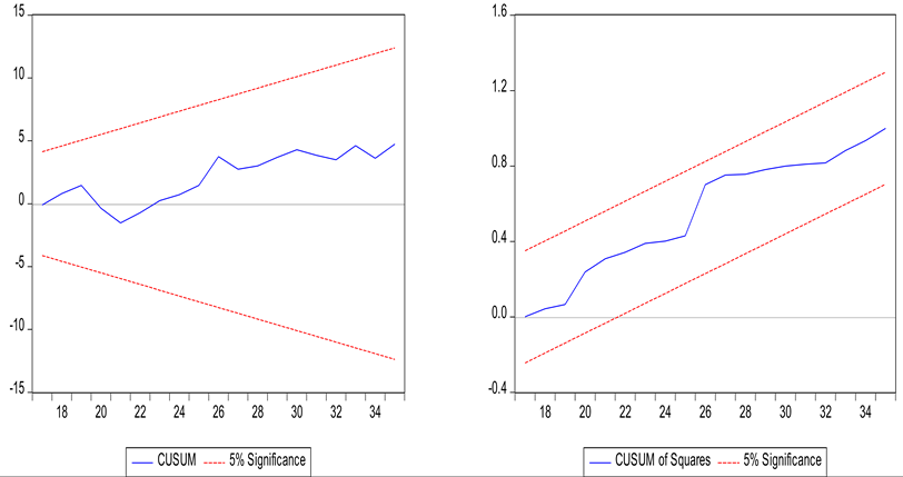 |
Table 8.
Results of short- run ARDL estimations.
Table 8.
Results of short- run ARDL estimations.
| Variables |
Coefficient |
Std. Error |
t-Statistic |
Prob.* |
| GDP(-1) |
0.2258 |
0.0996 |
2.2657 |
0.035** |
| GDP(-2) |
-0.3823 |
0.0988 |
-3.8676 |
0.001*** |
| FD |
0.1500 |
0.1452 |
1.0330 |
0.314 |
| FD(-1) |
-0.2965 |
0.1220 |
-2.4304 |
0.025** |
| HC |
0.3324 |
0.6441 |
0.5161 |
0.611 |
| HC(-1) |
-1.4649 |
0.6655 |
-2.2010 |
0.040** |
| HC(-2) |
2.1632 |
0.6546 |
3.3041 |
0.003*** |
| GOVE |
0.0622 |
0.0308 |
2.0186 |
0.057* |
| EP |
0.2441 |
0.1319 |
1.8496 |
0.080* |
| EP(-1) |
0.1729 |
0.1744 |
0.9912 |
0.334 |
| EP(-2) |
-0.4402 |
0.1507 |
-2.9195 |
0.008*** |
| OPV |
0.0976 |
0.0209 |
4.6737 |
0.000*** |
| OPV(-1) |
-0.1364 |
0.0273 |
-4.9799 |
0.000*** |
| OPV(-2) |
0.0645 |
0.0169 |
3.8070 |
0.001*** |
Table 9.
Results of long- run ARDL estimations.
Table 9.
Results of long- run ARDL estimations.
| Variables |
Coefficients |
Std. Error |
t-Statistic |
Prob. |
| FD |
-0.1266 |
0.0516 |
-2.4510 |
0.0241** |
| HC |
0.0891 |
0.0820 |
1.0857 |
0.0291** |
| GOVE |
0.0538 |
0.0266 |
2.0228 |
0.0574* |
| EP |
-0.0200 |
0.0202 |
-0.9888 |
0.3352 |
| OPV |
0.0223 |
0.0077 |
2.8804 |
0.0096*** |
|
Disclaimer/Publisher’s Note: The statements, opinions and data contained in all publications are solely those of the individual author(s) and contributor(s) and not of MDPI and/or the editor(s). MDPI and/or the editor(s) disclaim responsibility for any injury to people or property resulting from any ideas, methods, instructions or products referred to in the content. |
© 2025 by the authors. Licensee MDPI, Basel, Switzerland. This article is an open access article distributed under the terms and conditions of the Creative Commons Attribution (CC BY) license (http://creativecommons.org/licenses/by/4.0/).


