Fast Computation for Square Matrix Factorization

1. Introduction

The factorization of a matrix $A$ by an orthogonal (or unitary) matrix $Q$ and a triangular matrix $R$, which is known as the QR-factorization, or the QR-decomposition, is a fundamental technique which is widely used in various applications in computing and data analysis. This factorization is computationally effective in solving a large linear system $Ax=y$ (as $x=A^{-1}y$), to solve least squares problems [1]-[6], in signal and image processing [7,8], in image watermarking [9,10], in improving air traffic control radar [11], to analyze the stability of linear systems in control theory [12,13], in solving linear regression problems in machine learning [14,15], for linear programming algorithms [16], in quantum computing to build effective methods of calculation muti-qubit operations [17]-[20]. The matrix $A$ is presented as the product of two matrices, $A=QR$. The inverse matrix $A^{-1}$ is calculated as $A^{-1}=R^{-1}{Q}^{-1}=R^{-1}{Q}^{*}$. Here, $Q^{*}$ is the conjugate transpose to $Q$, and the inverse matrix $R^{-1}$ can be easily calculated, by using an iterative process called back substitution. The QR factorization is a well-known method in linear algebra, but how to implement this in the most efficient way for big data in computing is still a question.

Many methods of QR-factorization have been introduced for real matrices $A$, and then were modified for complex matrices. We mention the Gram-Schmidt process [21]-[23], the method of Householder reflections (or Householder transformations) [24]-[27], and the Givens rotations [28]-[31]. We consider the QR-factorization with an upper triangular matrix $R$ and will dwell on the factorization which is calculated by the discrete signal-induced heap transformations (DsiHT) [32]. For a real matrix, the DsiHT can be composed by the elementary rotations. Together with these 2×2 basic operations, the DsiHT is determined by the path, or order, of processing the signal components. The description of these transformations for two particular cases which are called the DsiHT with the weak and strong 2-wheel carriages has been given in [32,33]. These DsiHT are called the weak and strong DsiHT, respectively. The first transformation operates on the signal $\mathit{x}=(x_0,x_1,x_2,\dots ,x_{N-1})$ in the usual way, that is, the 2×2 rotations operate in the order $x_0$ and $x_1$, then the renewed $x_0$ and $x_2$, and so on. The strong DsiHT processes the signal components in the order $x_{N-2}$ and $x_{N-1}$, then $x_{N-3}$with the renewed $x_{N-2},$ and continuing in this manner, all the signal-generator energy is transferred to the first component of the transform. Every second output of the rotations is zeroed.

The present work is a continuation of the research in the QR-factorization of square matrices. From very beginning much attention was given to the path of the $N$-point DsiHT, especially for large $N$. Many paths can be chosen for the transformation and among them we are looking for paths which lead to effective calculation of the DsiHT-based QR-factorization. Each path of the transformation determines the structure of its matrix and the number of zero coefficients in it. Therefore, we are looking for paths that determines sparse matrices of the transformation. Such paths exist and they can be used instead of the paths in the above mentioned weak and strong DsiHTs. We present two such paths, which are call fast paths #3 and #4. The paths for the weak and strong DsiHT are referred to as paths #1 and #2, respectively. The DsiHTs with fast paths are defined by unitary matrices that are sparser than the matrices of the original two DsiHTs. For instance, the 256-point DsiHTs by the fast paths have 63,232 zero coefficients out of 65,536, whereas when using path #1 or #2, the number of zero coefficients is 32,325. It means that less operations are required to perform the transformation $H:\mathit{x}\to (‖\mathit{x}‖,0,\dots 0)$ and therefore, less operations to calculate the QR-factorization.

The main contributions of this work are the following:

• Description of the fast paths for the $N$-point DsiHT with a sparse matrix. For instance, when $N=2^r,r>2$, the matrix of the transformation has $N^2-N({\log }_{2}N+1)$ zero coefficients.
• The concept of the DsiHT with new 2$\times$2 complex matrices for the ‘complex Givens rotations.’
• The reduced number of multiplications in the QR-factorization.
• Algorithms with fast paths that allow us to perform all real and complex rotation in the QR-factorization only on the adjacent bit planes.
• Encoded tables with $N\left(N-1\right)/2$ angles for the real unitary matrix $Q$. Such tables can be used to generate random unitary $N\times N$ matrices.
• Illustrative examples that show advantage of using the DsiHT with fast paths when comparing with the Housholder reflection-based QR-factorization.

The rest of the paper is organized in the following way. In Section II, the concept of the $N$-point DsiHT is described with examples of different paths for the $N=4$ case. The comparison with the method of the Housholder reflections is also given. Section 3 describes all $N$-points DsiHTs with fast paths for $N\le 8.$ The matrices of the DsiHTs with five different paths are given and compared with the 8-point Housholder reflection. The algorithm for the $N$-points DsiHT with fast path #4 is also presented in the general case, when $N>2$. In Section 4, the DsiHT-based QR-factorization is described with the example for a 5$\times$5 real matrix. The concept of the complex DsiHT with the fast paths and different 2$\times$2 basic operations is presented in Section 5. Examples with 5$\times$5 and 256$\times$256 complex matrices are described and compared with the Housholder reflection-based QR-factorization calculated in MATLAB.

2. QR-Factorization

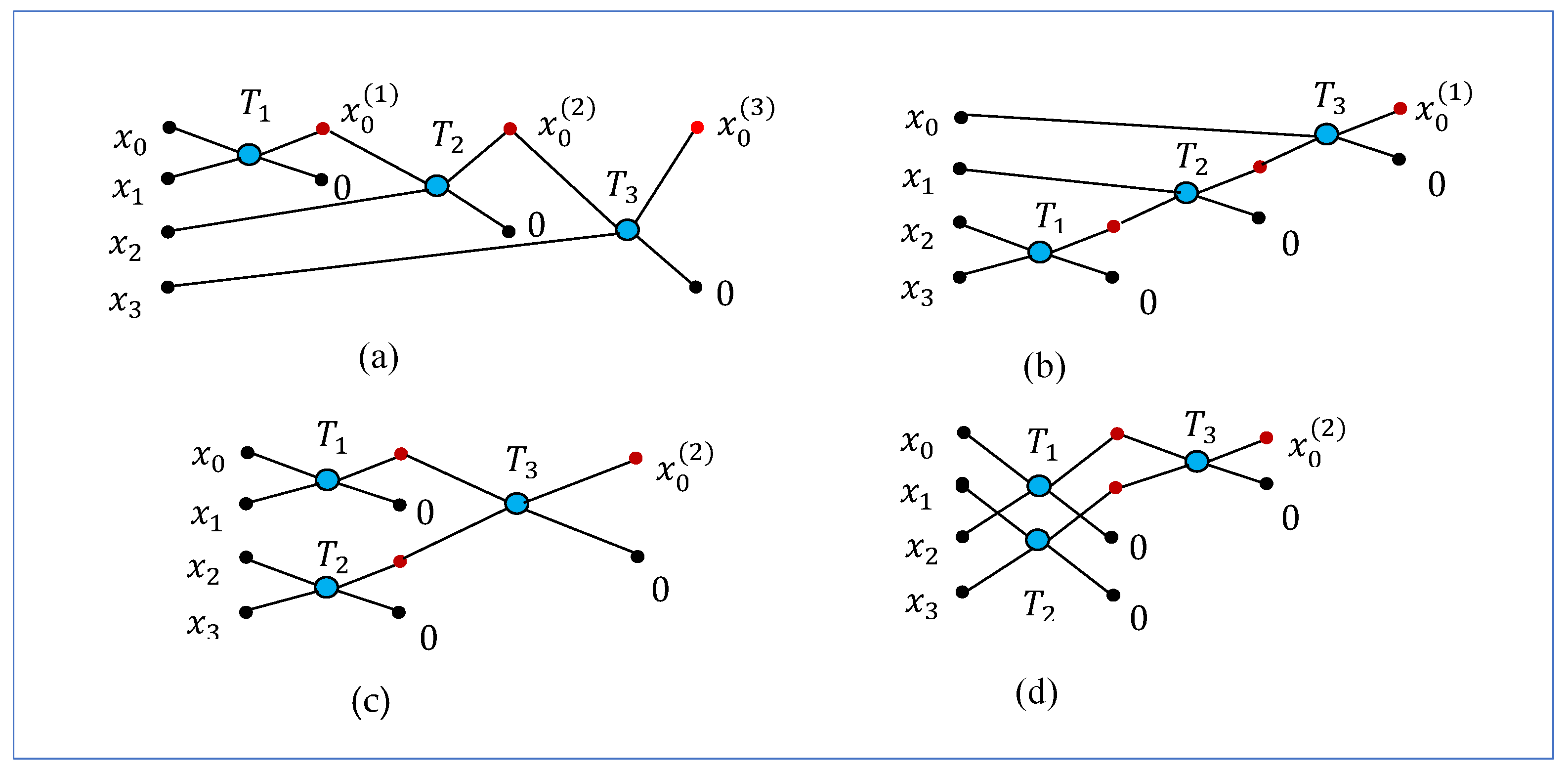
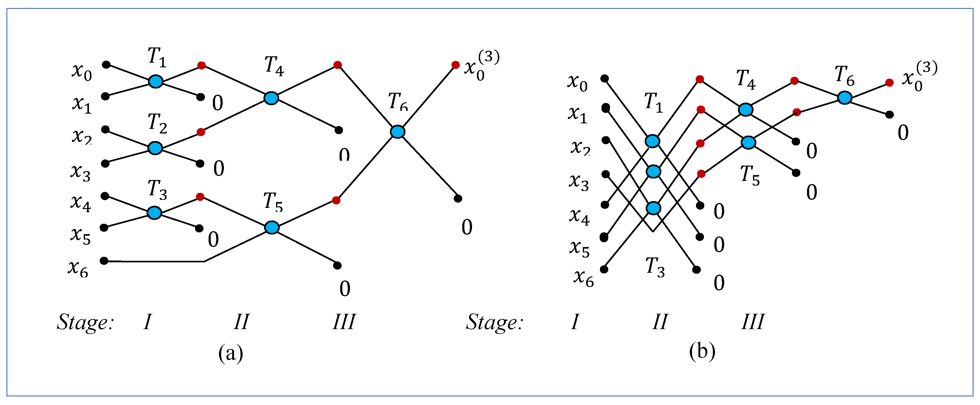
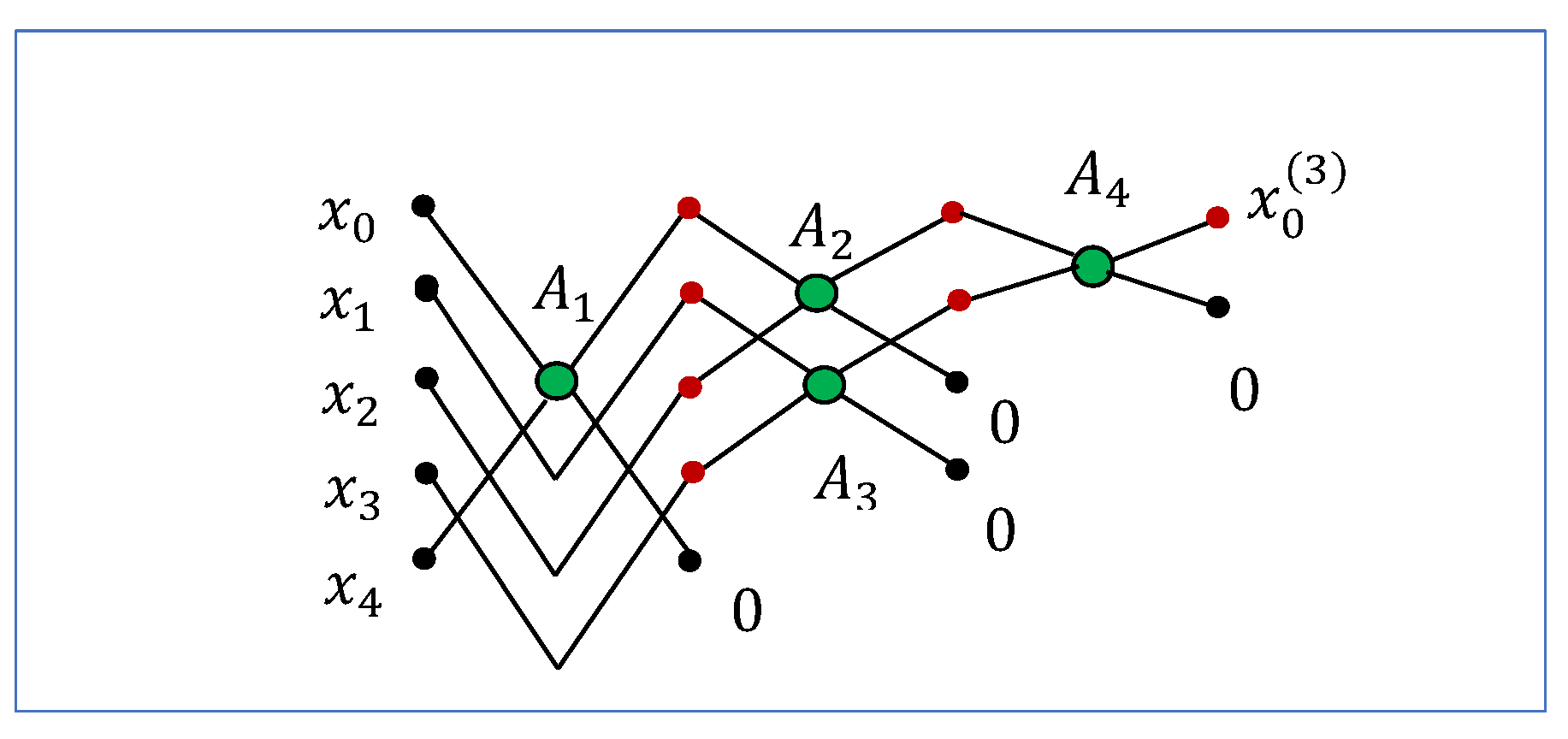
In this section, we consider the $N$-point DsiHT for the case when $N$ is equal to or differs from a power of 2. The transformation requires $(N-1)$ elementary rotations [32]. There are many ways to calculate the transform. As example, we consider the 4-point DsiHTs which are defined by the diagrams shown in Figure 1. The signal is considered real. These diagrams show different orders, or paths, to process the components of the input. In part (a), the components $x_0,x_1,x_2,$ and $x_3$ of the input signal (generator) $\mathit{x}$ are processed in the natural order. This is the traditional path of processing the signal. The DsiHT with such a path is called the weak carriage-wheel DsiHT (see [32] for more detail). The first value of the transform is renewed three times. This is why it is denoted by $x_0^{\left(3\right)}$. Each 2-point unitary transform $T_k,$ $k=\mathrm{1,2},3$, is the Givens rotation, or elementary rotation. In the figure, these rotations are depicted as butterflies. In the matrix form, the rotation $T:\left(x,y\right)\to \left(\pm \sqrt{x^2+y^2},0\right)$ is described as

$$T\left[\begin{array}{c}x\\ y\end{array}\right]=\left[\begin{array}{cc}\cos \vartheta & -\sin \vartheta \\ \sin \vartheta & \cos \vartheta \end{array}\right]\left[\begin{array}{c}x\\ y\end{array}\right]=\left[\begin{array}{c}\pm \sqrt{x^2+y^2}\\ 0\end{array}\right].$$

(1)

The rotation angle is defined by the inputs as $\vartheta =-\arctan \left(y/x\right)$. If $x=0$, then $\vartheta =\pm \pi /2$. The transform of the generator ${\mathit{x}=(x}_0,x_1,x_2,x_3)$ is equal to

$$T\mathit{x}=\left(\pm ‖x‖,\mathrm{0,0},0\right)=\left(\pm \sqrt{x_0^2+x_1^2+x_2^2+x_3^2},\mathrm{0,0},0\right).$$

(2)

Thus, the energy $E\left[\mathit{x}\right]=‖\mathit{x}‖$ of the generator is transformed to the first component. The angles ${\vartheta }_k$, $k=\mathrm{0,1},2,$ are calculated from this generator. The set $A_x=\{{\vartheta }_1,{\vartheta }_2,{\vartheta }_3\}$ is called the angular representation of the signal-generator. Once the angles have been calculated, the transform of an input ${\mathit{z}=(z}_0,z_1,z_2,z_3)$ is calculated by using the same path,

$$T_1:\left(z_0,z_1\right)\to \left(z_0^{\left(1\right)},z_1^{\mathrm{\text{'}}}\right),T_2:\left(z_0^{\left(1\right)},z_2\right)\to \left(z_0^{\left(2\right)},z_2^{\mathrm{\text{'}}}\right),T_3:\left(z_0^{\left(2\right)},z_3\right)\to \left(z_0^{\left(3\right)},z_3^{\mathrm{\text{'}}}\right).$$

(3)

The result of the transformation is the signal $T\mathit{z}=\left(z_0^{\left(3\right)},z_1^{\text{'}},z_2^{\text{'}},z_3^{\text{'}}\right).$ The 4-point DsiHT is a unitary transform. Therefore, the energy of the signal is preserved, $E\left[\mathit{z}\right]=‖\mathit{z}‖=‖T\left(\mathit{z}\right)‖.$

Path #2 which is shown in the diagram in Figure 1 part (b) corresponds to the DsiHT which is called the strong carriage-wheel DsiHT [32]. Here, processing data starts with the last component $x_3$ of the signal. The first component $x_0$ is updated once at the end of the computation. Now, we consider two paths of the 4-point DsiHT shown in parts (c) and (d) in Figure 1. There are two different partitions of data on the first stage of computation. Two rotations $T_1$ and $T_2$ can be calculated in parallel. Total number of rotations, or butterflies, is equal to 3. We will call paths #3 and #4 of calculation shown in part (c) and (d), respectively, the fast paths. Of greatest interest are these two paths, which allow the calculation of the transform to be performed in two stages (or the minimum number of stages). Here, we also mention the following. Methods of QR-factorization by rotations are widely used in quantum computation to build quantum circuits for multi-qubit operations [33,34]. All rotations are required to operate on adjacent bit-planes (BP). Such bit-planes differ only in one bit. In the above case, when the signals are 4-point vectors (or 2-qubit superpositions), we can consider that the components $x_0,x_1,x_2,$ and $x_3$ lie on the bit-planes 0,1,2, and 3, that is 00, 01, 10, and 11, respectively. Three butterflies in the diagrams with fast paths operate only on adjacent BPs. For instance, the second butterfly $T_2$ operates on BPs (10) and (11) when using path #3, and on BP (01) and (11), when using path #4. For comparison, the butterfly $T_3$ in the diagram in part (a) operates on BPs (00) and (11), which are not adjacent BPs. Also, one can see that in the diagram in part (b), the second rotation $T_2$ operates on non-adjacent BPs (01) and (10). In general, for any integer $N>2$, we call the path of the $N$-point DsiHT the fast path, if all butterflies (rotations) operate only on adjacent BPs.

Example 1.

Let the generator be $\mathit{x}=(\mathrm{1,3},-\mathrm{2,5})$with the energy $E\left[\mathit{x}\right]=\sqrt{39}.$The matrices of the 4-point DsiHTs generated by$\mathit{x}$and four paths inFigure 1are the following:

$$H_{4;\#1}=\left[\begin{array}{rrrr}0.1601& 0.4804& -0.3203& 0.8006\\ -0.9487& 0.3162& 0& 0\\ 0.1690& 0.5071& 0.8452& 0\\ -0.2140& -0.6419& 0.4280& 0.5991\end{array}\right],\det H_{4;\#1}=1,$$

(4)

$$H_{4;\#2}=\left[\begin{array}{rrrr}0.1601& 0.4804& -0.3203& 0.8006\\ -0.9871& 0.0779& -0.0520& 0.1299\\ 0& 0.8736& 0.1807& -0.4519\\ 0& 0& 0.9285& 0.3714\end{array}\right],\det H_{4;\#2}=1,$$

(5)

$$H_{4;\#3}=\left[\begin{array}{rrrr}0.1601& 0.4804& -0.3203& 0.8006\\ -0.9487& 0.3162& 0& 0\\ 0.2727& 0.8181& 0.1881& -0.4702\\ 0& 0& 0.9285& 0.3714\end{array}\right],\det H_{4;\#3}=1,$$

(6)

$$H_{4;\#4}=\left[\begin{array}{rrrr}0.1601& 0.4804& -0.3203& 0.8006\\ -0.4176& 0.1842& 0.8351& 0.3070\\ 0.8944& 0& 0.4472& 0\\ 0& -0.8575& 0& 0.5145\end{array}\right],\det H_{4;\#4}=1.$$

(7)

The transforms $H_{4;\#\mathrm{k}}{\mathit{x}}^{\text{'}}={\left(\sqrt{39},\mathrm{0,0},0\right)}^{\text{'}},$ for $k=1:4.$ Each path determines the structure of the matrix. This can be well seen by the location and the number of zero coefficients in the above matrices. The number of zero coefficients in the first two matrices is equal to 3, and in the last two matrices this number is 4. The first rows in these matrices is the generator $\mathit{x}$ normalized to the coefficient of $0.1601$, that is, $\left(\mathrm{1,3},-\mathrm{2,5}\right)\times 0.1601.$ All numbers are given with an accuracy of 4 decimal places. The angles ${\vartheta }_k,k=\mathrm{1,2},3,$ (in degrees) for these transformations are given in Table 1.

For comparison, we consider the Householder transform matrix composed by the signal $\mathit{x}$, as follows [4,25]:

$$P_4=I_4-2{\displaystyle \frac{\mathit{v}{\mathit{v}}^{\text{'}}}{‖\mathit{v}‖}}=\left[\begin{array}{rrrr}-0.1601& -0.4804& 0.3203& -0.8006\\ -0.4804& 0.8011& 0.1326& -0.3315\\ 0.3203& 0.1326& 0.9116& 0.2210\\ -0.8006& -0.3315& 0.2210& 0.4475\end{array}\right],\det P_4=-1,$$

(8)

where $I_4$ is the 4$\times$4 identity matrix and the Householder vector $\mathit{v}$ is calculated as $v=\mathit{x}+‖\mathit{x}‖\left(\mathrm{1,0},\mathrm{0,0}\right)={\left(1+\sqrt{39},3,-\mathrm{2,5}\right)}^{\mathrm{\text{'}}}.$ This matrix is symmetric (without zero coefficients) and orthogonal, and $P_4\mathit{x}\mathrm{\text{'}}=(-\sqrt{39},\mathrm{0,0},0)\mathrm{\text{'}}.$All these five matrices are different. As an example, we consider the input signal $\mathit{z}=\left(1,-\mathrm{3,2},5\right)\mathrm{\text{'}}$. Then, we obtain the following five different transforms:

$$H_{4;\#1}\mathit{z}={\left(2.081666,-1.897367,0.338062,5.563486\right)}^{\text{'}},$$

(9)

$$H_{4;\#2}\mathit{z}={\left(2.081666,-0.675382,-4.518564,3.713907\right)}^{\text{'}},$$

(10)

$$H_{4;\#3}\mathit{z}={\left(2.081666,-1.897367,-4.156148,3.713907\right)}^{\text{'}},$$

(11)

$$H_{4;\#4}\mathit{z}={\left(2.081666,2.235191,1.788854,5.144958\right)}^{\text{'}},$$

(12)

$$P_4\mathit{z}={\left(-2.081666,-4.276053,2.850702,2.873246\right)}^{\text{'}}.$$

(13)

3. $\mathit{N}$-Point DsiHT, when $\mathit{N}\le 8$

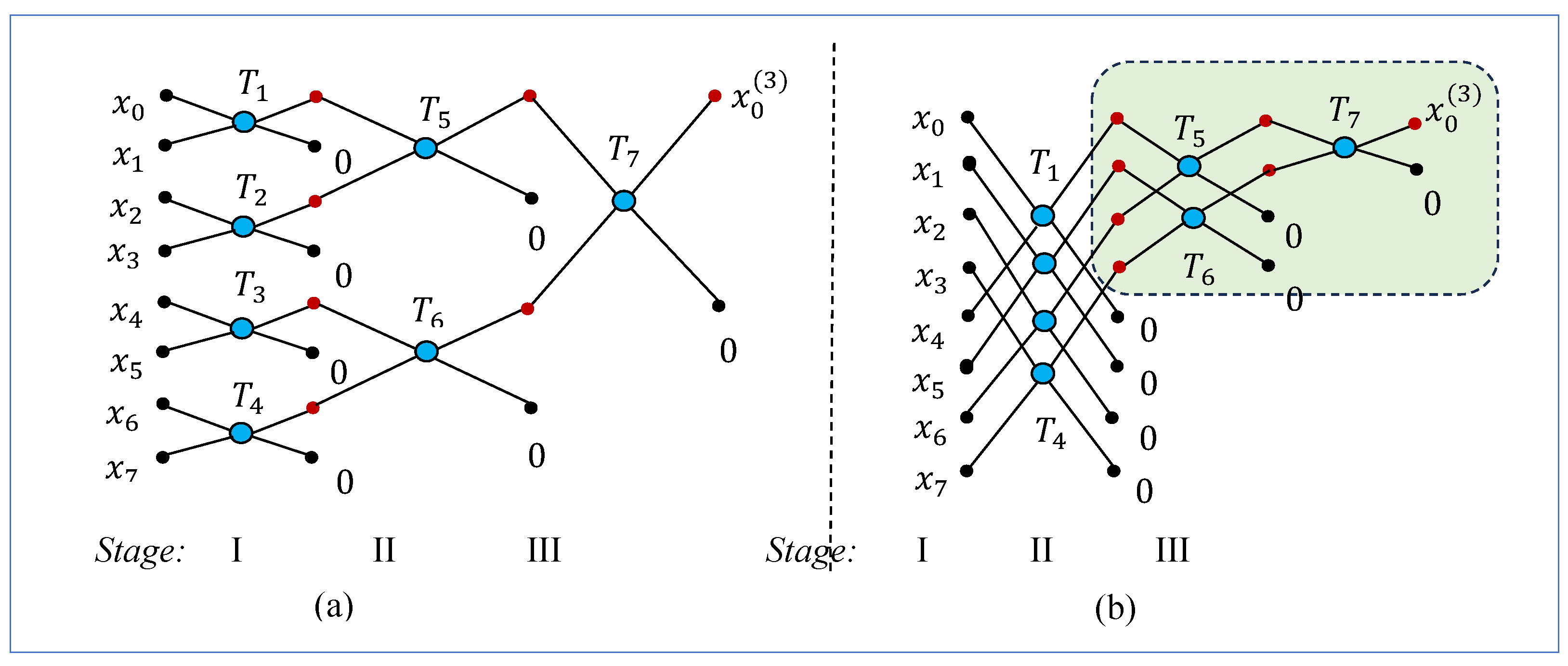
In this section, we describe $N$-point DsiHTs, starting from the number $N=8$ and reducing it to 3. For each of these transformations, we consider two fast paths, which are similar to the fast paths in Figure 1 in parts (c) and (d). First, we consider the 8-point DsiHTs with paths given in Figure 2. Seven butterflies are used in each of the diagrams shown in parts (a) and (b) and all butterflies operate on adjacent BPs. Four butterflies are used in the first stage, and they can be calculated in parallel. Two butterflies operate in the second stage, and one butterfly in the last stage. It is difficult to say which of these two paths is better. One can note in the diagram in part (b) that the calculations after Stage 1 represent the 4-point DsiHT described in Figure 1(d).

The paths which are similar to paths in Figure 1(a) and (b) can also be used for the 8-point DsiHT. It should be noted that, other fast paths exist for calculating the 8-point DsiHT. As an example, we consider the transformation with the diagram shown in Figure 3. The larger the value of $N$, the more paths can be found for computing the $N$-point DsiHT.

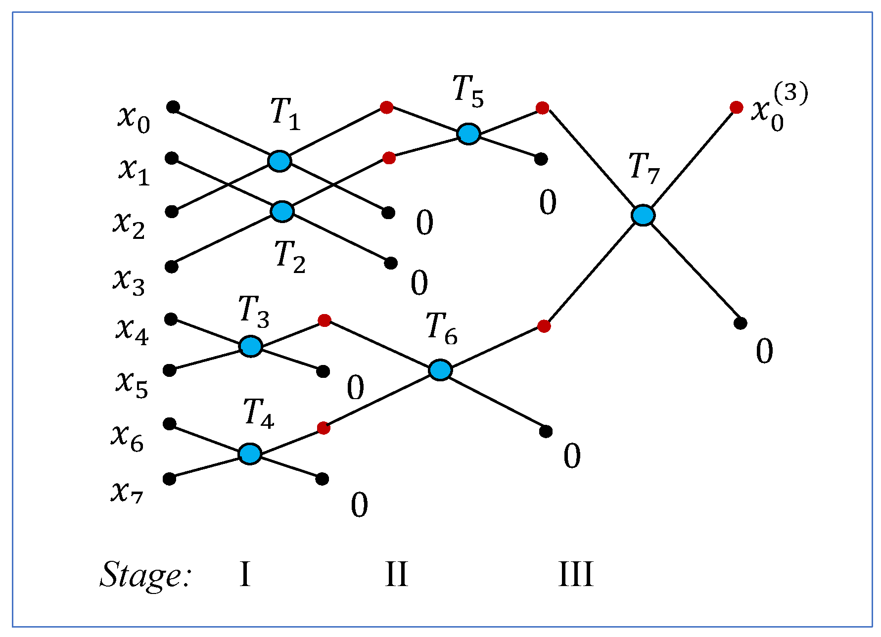
Example 2.

Let the generator be $\mathit{x}=(\mathrm{1,3},\mathrm{2,4},-2,-\mathrm{1,3},5)\text{'}$ with the energy $E\left[\mathit{x}\right]=\sqrt{69}.$ The matrices of the 8-point DsiHTs generated by $\mathit{x}$ and paths #1, 2, 3, and 4 are the following:

$$H_{8;\#1}=\left[\begin{array}{rrrrrrrr}0.1204& 0.3612& 0.2408& 0.4815& -0.2408& -0.1204& 0.3612& 0.6019\\ -0.9487& 0.3162& 0& 0& 0& 0& 0& 0\\ -0.1690& -0.5071& 0.8452& 0& 0& 0& 0& 0\\ -0.1952& -0.5855& -0.3904& 0.6831& 0& 0& 0& 0\\ 0.0626& 0.1879& 0.1252& 0.2505& 0.9393& 0& 0& 0\\ 0.0290& 0.0870& 0.0580& 0.1160& -0.0580& 0.9856& 0& 0\\ -0.0764& -0.2293& -0.1529& -0.3058& 0.1529& 0.0764& 0.8919& 0\\ -0.0907& -0.2722& -0.1815& -0.3630& 0.1815& 0.0907& -0.2722& 0.7985\end{array}\right],$$

(14)

$$H_{8;\#2}=\left[\begin{array}{rrrrrrrr}0.1204& 0.3612& 0.2408& 0.4815& -0.2408& -0.1204& 0.3612& 0.6019\\ -0.9927& 0.0438& 0.0292& 0.0584& -0.0292& -0.0146& 0.0438& 0.0730\\ 0& -0.9315& 0.0947& 0.1895& -0.0947& -0.0474& 0.1421& 0.2368\\ 0& 0& -0.9655& 0.1404& -0.0702& -00351& 0.1053& 0.1755\\ 0& 0& 0& 0.8421& 0.1727& 0.0864& -02591& -0.4318\\ 0& 0& 0& 0& -0.9473& 0.0541& -0.1624& -0.2707\\ 0& 0& 0& 0& 0& 0.9856& 0.0870& 0.1449\\ 0& 0& 0& 0& 0& 0& -0.8575& 0.5145\end{array}\right],$$

(15)

$$H_{8;\#3}=\left[\begin{array}{rrrrrrrr}0.1204& 0.3612& 0.2408& 0.4815& -0.2408& -0.1204& 0.3612& 0.6019\\ -0.9487& 0.3162& 0& 0& 0& 0& 0& 0\\ -0.2582& -0.7746& 0.2582& 0.5164& 0& 0& 0& 0\\ 0& 0& -0.8944& 0.4472& 0& 0& 0& 0\\ 0.1373& 0.4118& 0.2745& 0.5490& 0.2112& 0.1056& -0.3168& -0.5279\\ 0& 0& 0& 0& -0.4472& 0.8944& 0& 0\\ 0& 0& 0& 0& 0.8351& 0.4176& 0.1842& 0.3070\\ 0& 0& 0& 0& 0& 0& -0.8575& 0.5145\end{array}\right],$$

(16)

$$H_{8;\#4}=\left[\begin{array}{rrrrrrrr}0.1204& 0.3612& 0.2408& 0.4815& -0.2408& -0.1204& 0.3612& 0.6019\\ -0.2026& 0.2146& -0.4053& 0.2861& 0.4053& -0.0715& -0.6079& 0.3576\\ -0.3801& 0& 0.2924& 0& 0.7601& 0& 0.4385& 0\\ 0& -0.8506& 0& 0.2766& 0& 0.2835& 0& 0.3458\\ 0.8944& 0& 0& 0& 0.4472& 0& 0& 0\\ 0& 0.3162& 0& 0& 0& 0.9487& 0& 0\\ 0& 0& -0.8321& 0& 0& 0& 0.5547& 0\\ 0& 0& 0& -0.7809& 0& 0& 0& 0.6247\end{array}\right].$$

(17)

If we consider the 8-point DsiHT with path #5 shown in Figure 3, we obtain the following matrix of the transformation:

$$H_{8;\#5}=\left[\begin{array}{rrrrrrrr}0.1204& 0.3612& 0.2408& 0.4815& -0.2408& -0.1204& 0.3612& 0.6019\\ -0.4082& 0.2449& -0.8165& 0.3266& 0& 0& 0& 0\\ -0.8944& 0& 0.4472& 0& 0& 0& 0& 0\\ 0& -0.8000& 0& 0.6000& 0& 0& 0& 0\\ -0.1373& -0.4118& -0.2745& -0.5490& -0.2112& -0.1056& 0.3168& 0.5279\\ 0& 0& 0& 0& 0.4472& -0.8944& 0& 0\\ 0& 0& 0& 0& 0.8351& 0.4176& 0.1842& 0.3070\\ 0& 0& 0& 0& 0& 0& -0.8575& 0.5145\end{array}\right].$$

(18)

Each path defines the structure of the transformation matrix. The first rows in these matrices are the normalized generator $\mathit{x}$, that is, $\left(\mathrm{1,3},\mathrm{2,4}-2,-\mathrm{1,3},5\right)\times 0.1204,$ and $H_{8;\#\mathrm{n}}\mathit{x}=\left(\sqrt{69},\mathrm{0,0},\dots ,0\right)\text{'},n=1:5$. The angles ${\vartheta }_k,k=1:7,$ (in degrees) of rotations in these transformations are given in Table 2. The number of zero coefficients in these matrices is also shown in the table (in the last column)

Now, we consider the Householder transform matrix calculated as $P_8=I_8-2\mathit{v}{\mathit{v}}^{\text{'}}$/$‖\mathit{v}‖$ and equal to

$$P_8=\left[\begin{array}{rrrrrrrr}-0.1204& -0.3612& -0.2408& -0.4815& 0.2408& 0.1204& -0.3612& -0.6019\\ -0.3612& 0.8836& -0.0776& -0.1552& 0.0776& 0.0388& -0.1164& -0.1940\\ -0.2408& -0.0776& 0.9483& -0.1035& 0.0517& 0.0259& -0.0776& -0.1294\\ -0.4815& -0.1552& -0.1035& 0.7930& 0.1035& 0.0517& -0.1552& -0.2587\\ 0.2408& 0.0776& 0.0517& 0.1035& 0.9483& -0.0259& 0.0776& 0.1294\\ 0.1204& 0.0388& 0.0259& 0.0517& -0.0259& 0.9871& 0.0388& 0.0647\\ -0.3612& -0.1164& -0.0776& -0.1552& 0.0776& 0.0388& 0.8836& -0.1940\\ -0.6019& -0.1940& -0.1294& -0.2587& 0.1294& 0.0647& -0.1940& 0.6766\end{array}\right].$$

(19)

There is no zero coefficient in the matrix. The determinant of this matrix is equals to $-1$ and the transform $P_8\mathit{x}\mathrm{\text{'}}=(-\sqrt{69},0,\dots ,\mathrm{0,0})\mathrm{\text{'}}.$ The vector $v$ is calculated as $v=x+‖\mathit{x}‖\left(\mathrm{1,0},\dots ,\mathrm{0,0}\right)\mathrm{\text{'}}={\left(1+\sqrt{69},\mathrm{3,2},4,-2,-\mathrm{1,3},5\right)}^{\mathrm{\text{'}}}.$

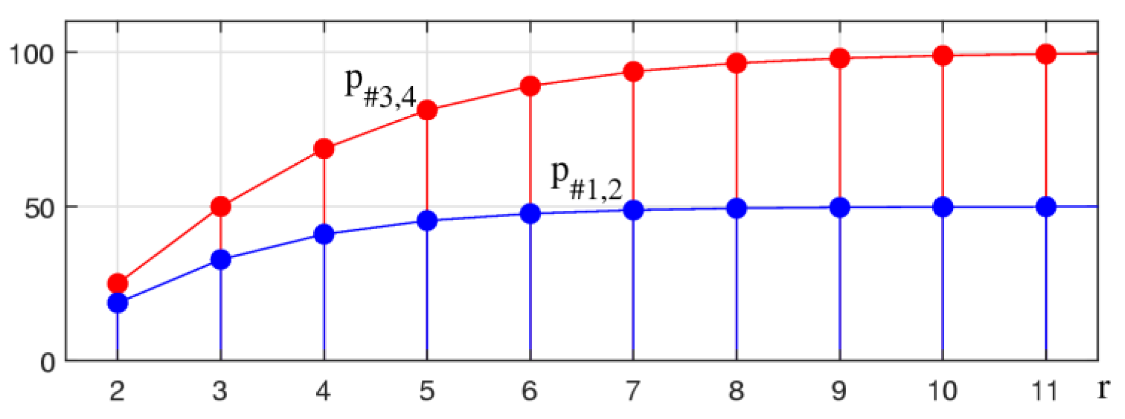
One can notice that the number of zero coefficients in the matrices $H_{8;\#3}$ and $H_{8;\#4}$ (and $H_{8;\#5}$) is much greater than in the matrices $H_{8;\#1}$ and $H_{8;\#2}$. These numbers are equal to 32 and 21, respectively. The number, $z_{\#\mathrm{1,2}}\left(N\right),$ of zero coefficients in the matrices $H_{N;\#1}$ and $H_{N;\#2}$ is the same. The same for the numbers, $z_{\#\mathrm{3,4}}\left(N\right),$ of zero coefficients in the matrices $H_{N;\#3}$ and $H_{N;\#4}$. In the case when $N=2^r,r\ge 2,$these numbers are calculated as follows:

$$z_{\#\mathrm{1,2}}(N)={\displaystyle \frac{\left(N-1\right)\left(N-2\right)}{2}},z_{\#\mathrm{3,4}}(N)=N^2-N\left({\log }_{2}N+1\right).$$

(20)

Figure 4 shows the graphs of these functions in percentage terms, for $N=2^r$, for $r=2:12$. That is, the number of zeros as a percentage of the matrix size $4^r$ is calculated for each of these functions,

$$p_{\#\mathrm{1,2}}\left(r\right)={z_{\#\mathrm{1,2}}\left(2^r\right)/4}^r\times 100\% \mathrm{and} p_{\#\mathrm{3,4}}\left(r\right)={z_{\#\mathrm{3,4}}\left(2^r\right)/4}^r\times 100\%$$

(21)

For comparison, the first nine values of these numbers are given in Table 3. The table also shows the difference $\mathsf{\Delta }z$ between the numbers $z_{\#\mathrm{3,4}}$ and $z_{\#\mathrm{1,2}}$ and their percentage to all $N^2$ coefficients in the matrices.

For $N=1024$, the difference of zero coefficients $z_{\#\mathrm{3,4}}$ and $z_{\#\mathrm{1,2}}$ is equal to 514,559. When multiplying matrices of the 1024-point DsiHT by a 1024-D vector $\mathit{z}$, the calculation requires ${1024}^2-z_{\#\mathrm{3,4}}\left(1024\right)=\mathrm{11,264}$ multiplications, if using the transforms with paths #3 and 4. For matrices with paths #1 and #2, the calculation requires ${1024}^2-z_{\#\mathrm{1,2}}\left(1024\right)=\mathrm{525,823}$ multiplications, or more than 46 times. In the general case of $N=2^r,r>2$, the number of multiplications when multiplying the matrices $H_{\#\mathrm{3,4}}$ by the vector $\mathit{z}$ is estimated as

$${\mu }_{\#\mathrm{3,4}}\left(N\right)=N^2-z_{\#\mathrm{3,4}}\left(N\right)=N\left({\log }_{2}N+1\right),$$

(22)

and when multiplying $H_{\#\mathrm{1,2}}$, the number of multiplications is estimated as

$${\mu }_{\#\mathrm{1,2}}\left(N\right)=N^2-z_{\#\mathrm{1,2}}\left(N\right)={\displaystyle \frac{1}{2}}\left(N^2+3N-2\right).$$

(23)

The number of operations saved when using the fast paths #3 and #4 is

$$\mathsf{\Delta }\mathrm{z}\left(N\right)=z_{\#\mathrm{3,4}}\left(N\right)-z_{\#\mathrm{1,2}}\left(N\right)={\displaystyle \frac{1}{2}}\left(N^2-N\left(2r-1\right)\right)+1.$$

(24)

These numbers are shown in the column number 4 in Table 3.

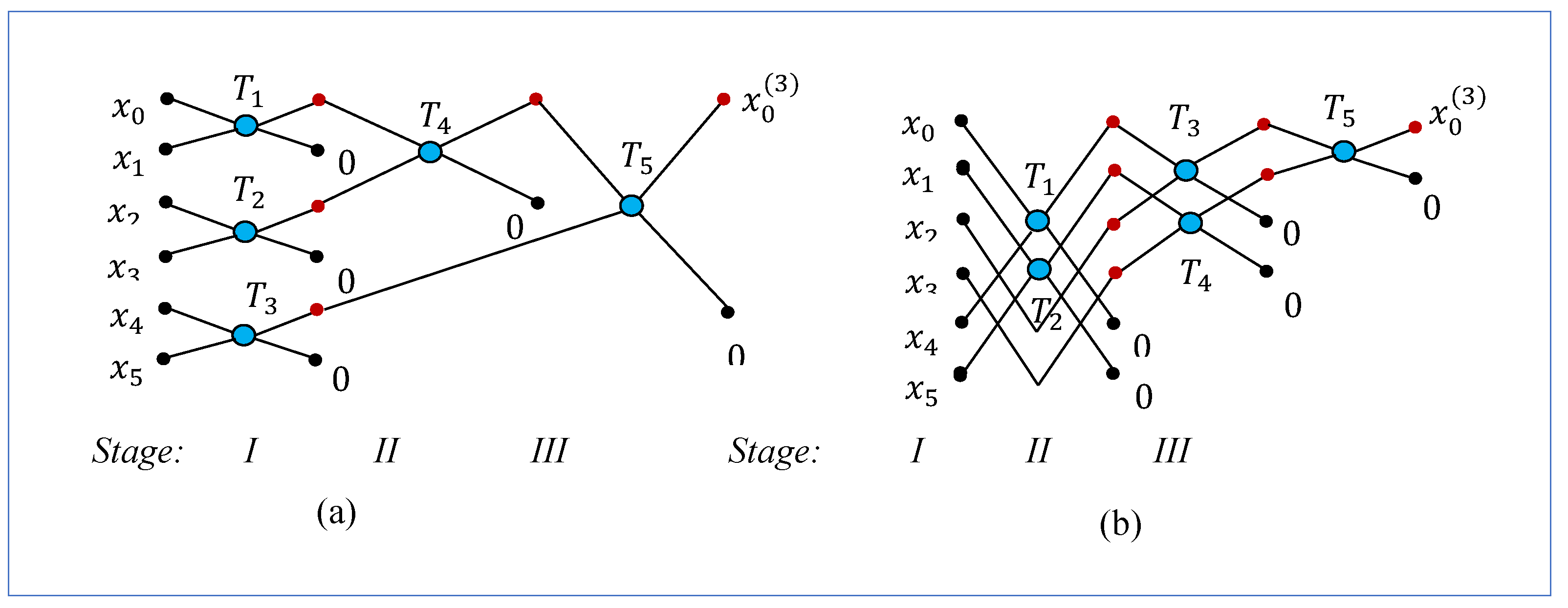
Next, we show that the diagrams of the 8-point DsiHT, which are shown in Figure 2 for two different paths, can be used and simplified when calculating the 7, 6, and 5-point DsiHTs, by removing the last inputs on the diagrams.

3.1. The $7$-Point DsiHT

Let us consider the $N=7$ case and the signal-generator $\mathit{x}=(x_0,x_1,\dots ,x_6)$. It is possible to consider the extended zero padded 8-D vector $\tilde{\mathit{x}}=(x_0,x_1,\dots ,x_6,0)$ and use the diagrams in Figure 2, after removing the rotations number 4 and then changing the numbers of the next three rotations. The corresponding diagrams are shown in Figure 5. On stage 1, three rotations are used. The total number of rotations is equal to six.

3.2. The $6$-Point DsiHT

The diagrams for calculating the 6-point DsiHTs by paths #3 and #4 are shown in Figure 6 in parts (a) and (b), respectively. For that, the diagrams in Figure 5 were used, after removing the last component $x_6$ from the input. In these two diagrams, the number of rotations on stages 1 and 2 are different. The total number of rotations is five.

3.3. The $5$-Point DsiHT

The last two simplifications of the diagrams of the 8-point DsiHT for the 5-point DsiHT are shown in Figure 7. Total four butterflies are used in both diagrams.

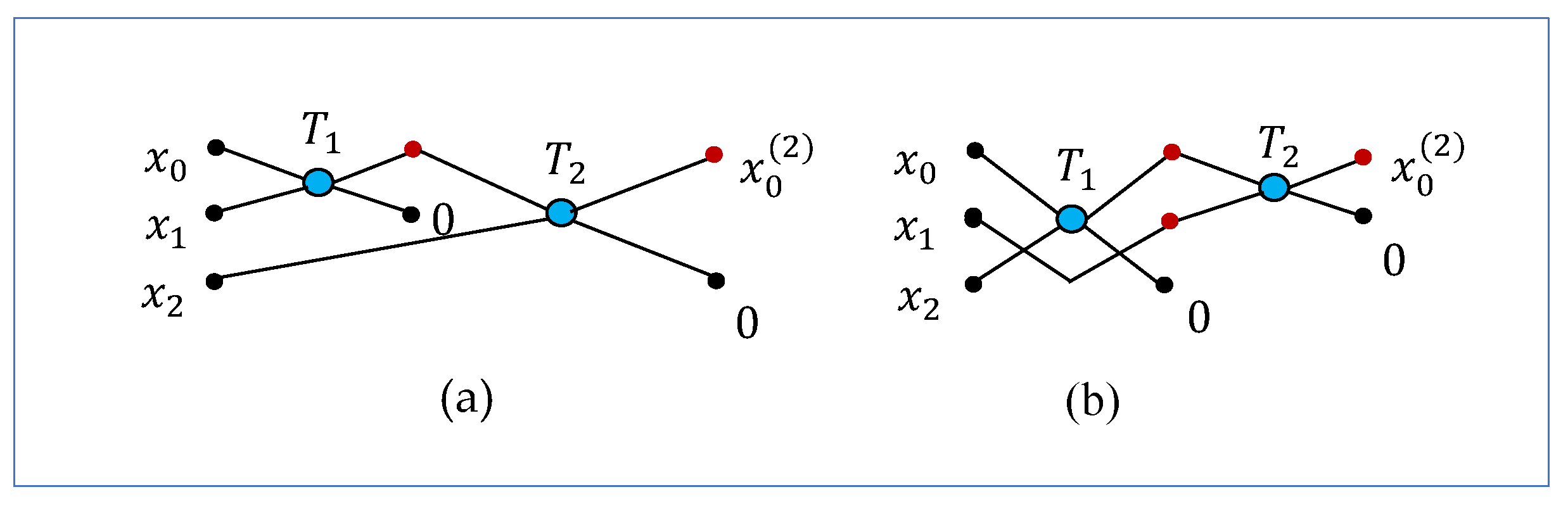
3.4. The $3$-Point DsiHT

The diagrams of the 4-point DsiHTs are given in Figure 1. For the 3-point DsiHT, there are only two paths can be considered. The diagrams with these paths are shown in Figure 8. Two butterflies are used for these transforms.

3.5. Algorithm of the DsiHT by Path #4

We stand on path #4, for any order $N$ of the DsiHT. The algorithm of the transformation with this path can be described as follows. Let us consider the smallest power of two, $M=2^n\ge N.$ The calculation of the transform generated by the signal $\mathit{x}=(x_0,x_1,\dots ,x_{N-1})$ can be performed in two steps as follows:

• The Givens rotations are applied to the pairs

$${R_{{\vartheta }_k}:(x}_k,x_{k+M/2})\to \left(x_k^{\mathrm{\text{'}}},0\right),k=\mathrm{0,1},\dots ,\left(N-{\displaystyle \frac{M}{2}}-1\right).$$

(25)

We will receive the signal $\mathit{y}=\left(\underbrace{x_0^{\text{'}},x_1^{\text{'}},\dots ,x_{N-M/2-1}^{\text{'}}},\underbrace{x_{N-M/2},\dots {,x}_{M/2-1}},\underbrace{\mathrm{0,0},\dots ,0}\right).$

2.

The $M/2$-point DsiHT with the fast path #4 is applied to the $M/2$2-point signal

$${\mathit{y}}_1=\left(\underbrace{x_0^{\mathrm{\text{'}}},x_1^{\mathrm{\text{'}}},\dots ,x_{N-M-1}^{\mathrm{\text{'}}}},\underbrace{x_{N-M/2},\dots ,x_{M/2-1}}\right).$$

(26)

The total number of rotations is equal to $(N-1)$.

As an example, we consider the diagram of the 7-point DsiHT, which is shown in Figure 5 part (b), when $N=7$. The first three rotations are applied to the pairs $(x_0,x_4)$, $(x_1,x_5)$, and $(x_2,x_6)$. Then, the first outputs of these rotations ${T_k:(x}_k,x_{k+4})\to {(x}_k^{\text{'}},0),k=\mathrm{0,1},2,$ together with the input component $x_3$ are used as the input signal, $\mathit{y}=\left(\underbrace{x_0^{\text{'}},x_1^{\text{'}},x_2^{\text{'}}},x_3\right)$, for the 4-point DsiHT. The composition of the 7-point DsiHT is described by the following six matrices of rotation:

$$H_{7;4}=T_6{T}_5{T}_4{T}_3{T}_2{T}_1={R_{{\vartheta }_{6;\left(\mathrm{0,1}\right)}}{R}_{{\vartheta }_{5;\left(\mathrm{1,3}\right)}}{R}_{{\vartheta }_{4;\left(\mathrm{0,2}\right)}}R}_{{\vartheta }_{3;\left(\mathrm{2,6}\right)}}{R}_{{\vartheta }_{2;\left(\mathrm{1,5}\right)}}{R}_{{\vartheta }_{1;\left(\mathrm{0,4}\right)}}.$$

(27)

Here, $R_{{\vartheta }_k;(i,j)}$, when $j\ne i$, denotes the matrix composed by the 7$\times$7 identity matrix [$a_{n,m};n,m=0:6$] and coefficients of the matrix rotation $R_{{\vartheta }_k}$ at the points (i,i), (i,$j$), ($j$,i), and ($j$, $j$). Thus,

$$H_{7;\#4}=\begin{array}{c}\left[\begin{array}{ccccccc}{c}_6& -s_6& 0& 0& 0& 0& 0\\ s_6& c_6& 0& 0& 0& 0& 0\\ 0& 0& 1& 0& 0& 0& 0\\ 0& 0& 0& 1& 0& 0& 0\\ 0& 0& 0& 0& 1& 0& 0\\ 0& 0& 0& 0& 0& 1& 0\\ 0& 0& 0& 0& 0& 0& 1\end{array}\right]\left[\begin{array}{ccccccc}1& 0& 0& 0& 0& 0& 0\\ 0& c_5& 0& {-s}_5& 0& 0& 0\\ 0& 0& 1& 0& 0& 0& 0\\ 0& s_5& 0& c_5& 0& 0& 0\\ 0& 0& 0& 0& 1& 0& 0\\ 0& 0& 0& 0& 0& 1& 0\\ 0& 0& 0& 0& 0& 0& 1\end{array}\right]\left[\begin{array}{ccccccc}{c}_4& 0& -s_4& 0& 0& 0& 0\\ 0& 1& 0& 0& 0& 0& 0\\ s_4& 0& c_4& 0& 0& 0& 0\\ 0& 0& 0& 1& 0& 0& 0\\ 0& 0& 0& 0& 1& 0& 0\\ 0& 0& 0& 0& 0& 1& 0\\ 0& 0& 0& 0& 0& 0& 1\end{array}\right]\\ \left[\begin{array}{ccccccc}1& 0& 0& 0& 0& 0& 0\\ 0& 1& 0& 0& 0& 0& 0\\ 0& 0& c_3& 0& 0& 0& -s_3\\ 0& 0& 0& 1& 0& 0& 0\\ 0& 0& 0& 0& 1& 0& 0\\ 0& 0& 0& 0& 0& 1& 0\\ 0& 0& s_3& 0& 0& 0& c_3\end{array}\right]\left[\begin{array}{ccccccc}1& 0& 0& 0& 0& 0& 0\\ 0& c_2& 0& 0& 0& -s_2& 0\\ 0& 0& 1& 0& 0& 0& 0\\ 0& 0& 0& 1& 0& 0& 0\\ 0& 0& 0& 0& 1& 0& 0\\ 0& s_2& 0& 0& 0& c_2& 0\\ 0& 0& 0& 0& 0& 0& 1\end{array}\right]\left[\begin{array}{ccccccc}{c}_1& 0& 0& 0& -s_1& 0& 0\\ 0& 1& 0& 0& 0& 0& 0\\ 0& 0& 1& 0& 0& 0& 0\\ 0& 0& 0& 1& 0& 0& 0\\ s_1& 0& 0& 0& c_1& 0& 0\\ 0& 0& 0& 0& 0& 1& 0\\ 0& 0& 0& 0& 0& 0& 1\end{array}\right].\end{array}$$

(28)

where $c_k=\cos {\vartheta }_k$ and $s_k=\sin {\vartheta }_k$, $k=1:6.$ The transform of the signal-generator $\mathit{x}$ is the vector

$$H_7\mathit{x}=\left(x_0^{\left(k\right)},\mathrm{0,0},\mathrm{0,0},\mathrm{0,0}\right)=\left(\sqrt{x_0^2+x_1^2+\dots +x_6^2},\mathrm{0,0},\mathrm{0,0},\mathrm{0,0}\right).$$

(29)

3.6. Number of Zero Coefficients in the DsiHT Matrices

For the $N$-point DsiHT calculated by paths #3 and 4, the number $z\left(N\right)$ of zero coefficients is estimated as follows. If $2^r\le N<2^{r+1}$, where $r\ge 2,$ the following recurrence formula is valid:

$$z\left(N+1\right)=z\left(N\right)+2N-\left(r+4\right).$$

(30)

In other words, in the $\left(N+1\right)\times (N+1)$ matrix of the $(N+1)$-point DsiHT there is $2N-\left(r+4\right)$ more zero coefficients than in the matrix of the $N$-point DsiHT. If we denote $N=2^r+n,$ where $n\in \left\{\mathrm{1,2},\dots ,2^r\right\},$ then the number $z\left(N\right)$ can be calculated as

$$z\left(N\right)=z_{\#\mathrm{3,4}}\left(2^r\right)+2^{r+1}n+n\left(n-r-3\right)={4^r+2}^r\left(2n-r-1\right)+n\left(n-r-3\right).$$

(31)

If $N=2^r$, then $z\left(N\right)=z_{\#\mathrm{3,4}}\left(N\right)$ calculated by Equation (20). A few values of these numbers are shown in Table 4.

The number of multiplications when multiplying the matrices $H_N$ by the $N$-dimensional vector $\mathit{z}$ can be estimated as $\mu \left(N\right)=N^2-z\left(N\right).$ These numbers are also given in Table 4 along with the maximum number of multiplications $N^2$ for comparison. Note that for the $N$-point DsiHT with path #1, the number of zero coefficients is calculated by $z_{\mathrm{1,2}}\left(N\right)=\left(N^2-3N+2\right)/2$, for any $N\ge 3.$

4. DsiHT-Based QR Factorization

In this section, we describe the QR-factorization of a square matrix $A$ of size $N\times N,N\ge 3,$ by the Givens rotations. The unitary matrix $A$ is considered with real coefficients. In the QR- factorization, $(N-1)$ DsiHTs are used. This factorization is illustrated below for a $5\times 5$ unitary matrix,

$$\begin{gathered} \left[\begin{array}{ccccc}\circ & \circ & \circ & \circ & \circ \\ \circ & \circ & \circ & \circ & \circ \\ \circ & \circ & \circ & \circ & \circ \\ \circ & \circ & \circ & \circ & \circ \\ \circ & \circ & \circ & \circ & \circ \end{array}\right]\stackrel{\circ :}{\to }\left[\begin{array}{ccccc}\star & \star & \star & \star & \star \\ 0& \star & \star & \star & \star \\ 0& \star & \star & \star & \star \\ 0& \star & \star & \star & \star \\ 0& \star & \star & \star & \star \end{array}\right]\stackrel{\star :}{\to }\left[\begin{array}{ccccc}\star & \star & \star & \star & \star \\ 0& \diamond & \diamond & \diamond & \diamond \\ 0& 0& \diamond & \diamond & \diamond \\ 0& 0& \diamond & \diamond & \diamond \\ 0& 0& \diamond & \diamond & \diamond \end{array}\right] \\ \stackrel{\diamond :}{\to }\left[\begin{array}{ccccc}\star & \star & \star & \star & \star \\ 0& \diamond & \diamond & \diamond & \diamond \\ 0& 0& \mathrm{*}& \mathrm{*}& \mathrm{*}\\ 0& 0& 0& \mathrm{*}& \mathrm{*}\\ 0& 0& 0& \mathrm{*}& \mathrm{*}\end{array}\right]\stackrel{\mathrm{*}:}{\to }\left[\begin{array}{ccccc}\star & \star & \star & \star & \star \\ 0& \diamond & \diamond & \diamond & \diamond \\ 0& 0& \mathrm{*}& \mathrm{*}& \mathrm{*}\\ 0& 0& 0& △& △\\ 0& 0& 0& 0& △\end{array}\right]. \end{gathered}$$

(32)

$A{A}_1{A}_2{A}_{3}R$The first 5-point DsiHT, $H_5,$ is generated by the first column of the matrix $A$ and then it is applied to each of its columns. Four zero coefficients will be obtained in the new matrix $A_1$ in its first column, as shown above. A similar transform will be applied on the 4$\times$4 submatrix (highlighted in red) of $A_1$. Namely, the 4-point DsiHT, $H_4$, will be generated by the last four components of the second column of the matrix $A_1$. This transform will be applied to each column of the 4$\times$4 submatrix.

In the new matrix $A_2$, another three zero coefficients in the 2^nd column will be obtained. Then, the 3-point DsiHT, $H_3$, will be generated by the first column of the 3$\times$3 sub-matrix of $A_2$ and applied on this sub-matrix. We will obtain a new matrix $A_3$ with 9 zero coefficients, as shown in Equation (32). The last 2-point DsiHT, $H_2$, will be generated by the last two coefficients of the 4^th column of $A_3$ and applied to its 2$\times$2 sub-matrix. Thus, the matrix triangularization is completed as

$$R=\left(I_3\oplus H_2\right)\left(I_2\oplus H_3\right)\left(1\oplus H_4\right)H_{5}A.$$

(33)

Here, $I_n$ is the identity $n\times n$ matrix. If we denote the unitary matrix $Q_1=\left(I_3\oplus H_2\right)\left(I_2\oplus H_3\right)\left(1\oplus H_4\right)H_5$ and its inverse

$$Q=Q_1^{-1}=Q_1^{\mathrm{\text{'}}}=H_5^{\mathrm{\text{'}}}\left(1\oplus H_4^{\mathrm{\text{'}}}\right)\left(I_2\oplus H_3^{\mathrm{\text{'}}}\right)\left(I_3\oplus H_2^{\mathrm{\text{'}}}\right),$$

(34)

then, we can write $A=QR.$ This is the result of the QR-factorization. The matrix $R$ is upper-triangular and $Q$ is the unitary matrix. The matrix operation ‘$\text{'}$’ stands for the matrix transposition.

Let us estimate the number $m\left(5\right)$ of multiplications in the QR-factorization of the 5$\times$5 matrix $A$. The first 5-point DsiHT is applied to five columns of $A$. Then, the second 4-point DsiHT is applied to four columns of the 4$\times$4 submatrix of $A_1$, and so on. Thus, considering the number of zero coefficients in the matrices of the DsiHTs, we obtain the following estimation:

$$m\left(5\right)=5\mu \left(5\right)+4\mu \left(4\right)+3\mu \left(3\right)+2\mu \left(2\right)=5\cdot 17+4\cdot 12+3\cdot 8+2\cdot 4=165.$$

(35)

The number of rotations that perform the QR-factorization of the matrix is equal to $\alpha \left(N\right)=4+3+2+1=10.$ If use the Householder transformations in the QR- factorization of the same 5$\times$5 matrix, the number of multiplications will be estimated by $5\cdot 25+4\cdot 16+3\cdot 9+2\cdot 4=224.$

Example 2.

Consider the following randomly generated 5$\times$5 matrix:

$$A=\left[\begin{array}{rrrrr}4& 3& 1& 5& -6\\ 8& 1& -3& 5& 9\\ -7& 6& 2& 8& 3\\ 9& 8& 3& -5& 7\\ 5& 4& -2& 9& 3\end{array}\right],\det A\ne 0.$$

(36)

The QR-factorization of the matrix, $A\to R$, where the upper triangular matrix $R={{H_{2}H}_{3}H}_4{H}_{5}A$, is calculated as follows. The first 5-point DsiHT with fast path #4 is generated by the column $x=\left(\mathrm{4,8},-\mathrm{7,9},5\right)\text{'}.$ The matrix in this factorization is equal to

$$H_5=\left[\begin{array}{rrrrr}0.2609& 0.5219& -0.4566& 0.5871& 0.3262\\ -0.3312& 0.4111& 0.5796& 0.4625& -0.4140\\ 0.4609& 0& 0.6749& 0& 0.5762\\ 0& -0.7474& 0& 0.6644& 0\\ -0.7809& 0& 0& 0& 0.6247\end{array}\right],\det H_4=1.$$

(37)

At the next three stages of the matrix factorization, the matrices are composed by the matrices of the 4-,3-, and 2-point DsiHTs and are equal to

$$H_4=\left[\begin{array}{rrrrr}1& 0& 0& 0& 0\\ 0& 0.4817& 0.7545& 0.4454& 0.0152\\ 0& -0.5541& 0.6559& -0.5124& 0.0132\\ 0& -0.6789& 0& 0.7342& 0\\ 0& 0& -0.0202& 0& 0.9998\end{array}\right],\det H_4=1,$$

(38)

and

$$H_3=\left[\begin{array}{rrrrr}1& 0& 0& 0& 0\\ 0& 1& 0& 0& 0\\ 0& 0& 0.7060& -0.4796& 0.5211\\ 0& 0& 0.3859& 0.8775& 0.2848\\ 0& 0& -0.5939& 0& 0.8046\end{array}\right],H_2=\left[\begin{array}{rrrrr}1& 0& 0& 0& 0\\ 0& 1& 0& 0& 0\\ 0& 0& 1& 0& 0\\ 0& 0& 0& 0.2077& -0.9782\\ 0& 0& 0& 0.9782& 0.2077\end{array}\right].$$

(39)

The unitary matrix $Q$ is calculated as $Q={\left({{H_{2}H}_{3}H}_4{H}_5\right)}^{\mathrm{\text{'}}}=H_5^{\mathrm{\text{'}}}{H}_4^{\mathrm{\text{'}}}{H}_3^{\mathrm{\text{'}}}{H}_2^{\mathrm{\text{'}}}$ and is equal to

$$Q=\left[\begin{array}{rrrrr}0.2609& 0.1764& -0.1838& 0.9304& -0.0383\\ 0.5219& -0.1349& 0.5066& -0.0483& -0.6712\\ -0.4566& 0.7885& 0.2675& 0.0186& -0.3129\\ 0.5871& 0.5187& -0.5046& -0.3628& -0.0025\\ 0.3262& 0.2448& 0.6192& 0.0121& 0.6709\end{array}\right],\det Q=1.$$

(40)

The triangular matrix is

$$R=Q^{\mathrm{\text{'}}}A=\left[\begin{array}{rrrrr}15.3297& 4.5663& -1.1090& 0.2609& 6.8494\\ 0& 10.2542& 3.2244& 6.1251& 4.4590\\ 0& 0& -3.9209& 11.8495& 4.7902\\ 0& 0& 0& 6.4810& -8.4648\\ 0& 0& 0& 0& -4.5743\end{array}\right].$$

(41)

Ten angles of rotations in these four DsiHTs are given in Table 5 (in degrees). This is an encoded table of the QR-factorization by the DsiHTs with path #4.

We remind that in the QR-factorization, the triangularization $T:A\to R$ is accomplished by a unitary matrix $Q$. The original matrix is integer-valued, and it always possible to fulfil the triangularization by the integer matrices only, as shown below

$$R_i=TA=\left[\begin{array}{rrrrr}2& 0& 1& 0& 0\\ -12& 11& 5& 0& -1\\ -33& 1& -1& 13& 0\\ 1& 15& 7& 0& -15\\ 153& 2681& 1250& 10& -2680\end{array}\right]A=\left[\begin{array}{rrrrr}1& 12& 4& 18& -9\\ 0& 1& -33& 26& 183\\ 0& 0& 1& -233& 295\\ 0& 0& 0& 1& 105\\ 0& 0& 0& 0& 18991\end{array}\right].$$

(42)

The determinant of the matrix $T$ is equal to $\det T=1$, but this matrix is not unitary. To calculate the matrix $A$ from this equation as $A=T^{-1}{R}_i$, the inverse of the matrix $T^{-1}$ is required, which is not the transpose matrix, that is, ${Q=T}^{-1}\ne T\text{'}.$The QR-factorization of the same matrix $A$ by the Householder reflections results in the matrices

$$Q=\left[\begin{array}{rrrrr}-0.2609& -0.1764& -0.1838& -0.9304& 0.0383\\ -0.5219& 0.1349& 0.5066& -0.0483& 0.6712\\ 0.4566& -0.7885& 0.2675& -0.0186& 0.3129\\ -0.5871& -0.5187& -0.5046& 0.3628& 0.0025\\ -0.3262& -0.2448& 0.6192& -0.0121& -0.6709\end{array}\right],\det Q=1,$$

(43)

and

$$R=\left[\begin{array}{rrrrr}-15.3297& -4.5663& 1.1090& -0.2609& -6.8494\\ 0& -10.2542& -3.2244& -6.1251& -4.4590\\ 0& 0& -3.9209& 11.8495& 4.7902\\ 0& 0& 0& -6.4810& 8.4648\\ 0& 0& 0& 0& 4.5743\end{array}\right].$$

(44)

It can be noted that the coefficients of these matrices differ only in signs from the corresponding matrices of the DsiHT-based QR factorization, given in Equations (40) and (41). This example illustrates the advantage of the DsiHT-based method over the Householder reflection method. The results are almost the same, but the DsiHTs reduce the operations of multiplication by the number $224-165=59$, plus the encoded QR-factorization table is generated. Such a table can be used to create a unitary matrix 5$\times$5.

The numbers of operations of multiplication for the QR-factorization by the Housholder reflections and DsiHT with paths #1 and #4, are calculated as

$$m_H\left(N\right)=2^3+3^3+4^3+\dots +N^3={\displaystyle \frac{1}{4}}{N}^2{\left(N+1\right)}^2-1,\left(45\right)$$

(45)

$$\begin{gathered} m_{\#\mathrm{1,2}}\left(N\right)=\sum _{n=2}^{N}n{\mu }_{\#\mathrm{1,2}}\left(n\right)=\sum _{n=2}^{N}n{\displaystyle \frac{1}{2}}\left(n^2+3n-2\right)={\displaystyle \frac{1}{2}}\sum _{n=2}^N\left(n^3+3n^2-2n\right) \\ ={\displaystyle \frac{1}{8}}\left[N^2{\left(N+1\right)}^2-4\right]+{\displaystyle \frac{1}{4}}\left[N\left(N+1\right)\left(2N+1\right)-6\right] \\ -{\displaystyle \frac{1}{2}}\left(N+2\right)\left(N-1\right), \end{gathered}$$

(46)

$$m_{\#\mathrm{3,4}}\left(N\right)=\sum _{n=2}^{N}n{\mu }_{\#\mathrm{3,4}}\left(n\right)=\sum _{k=2}^{N}n\left(n^2-z_{\#\mathrm{3,4}}\left(n\right)\right),$$

(47)

where $z_{\#\mathrm{3,4}}\left(n\right)=z\left(n\right)$ is calculated by Equation (31). The values of these estimations for small values of $N=3:14$ and for powers of two, $128,\mathrm{256,512,1024},$and $2048$, are given in Table 6.

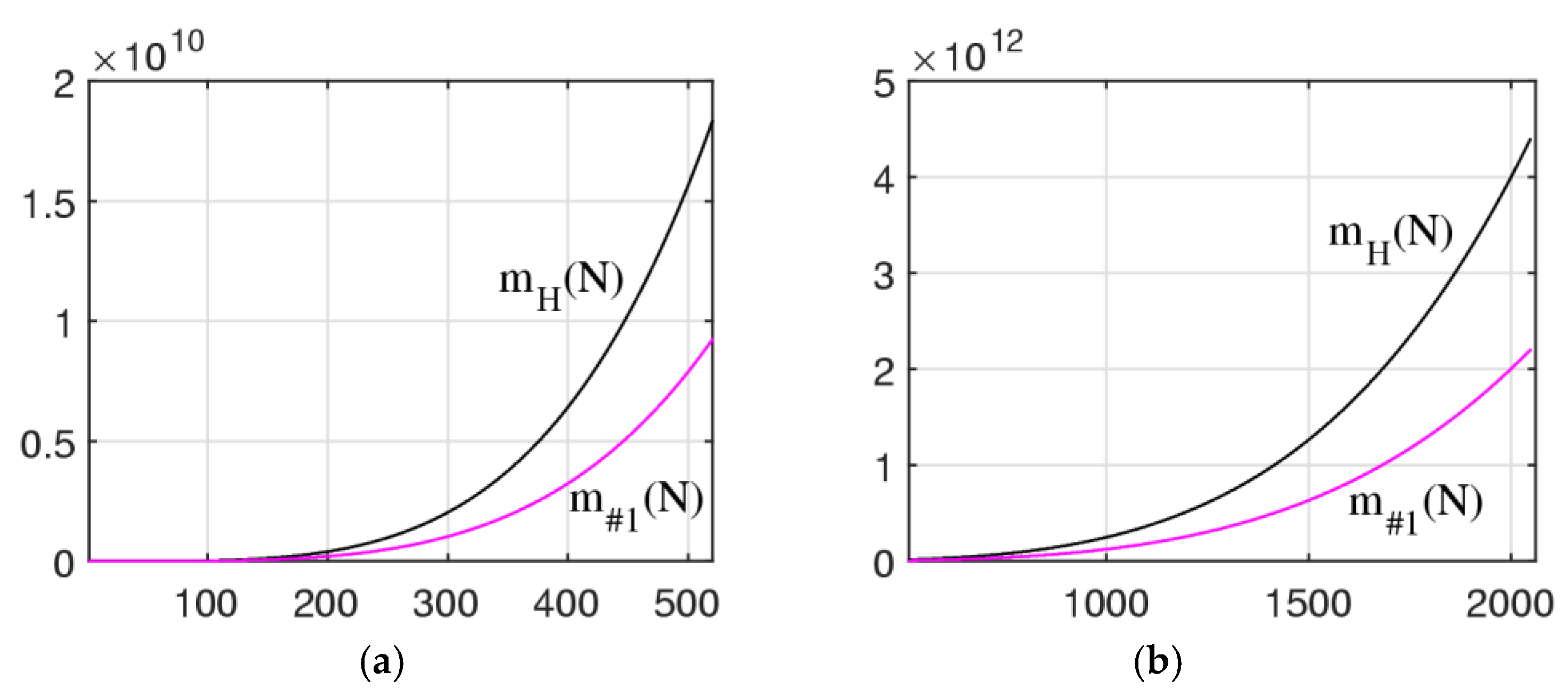
One can note that the DsiHT-based method with the fast path #4 required a smaller number of multiplications when comparing with the path #1, as well as the Householder reflection-based method. The graphs of the functions $m_H\left(N\right)$ and $m_{\#1}\left(N\right)$ are shown in Figure 9 in part (a), when $N=3:512$, and in part (b) when $N=512:2048$.

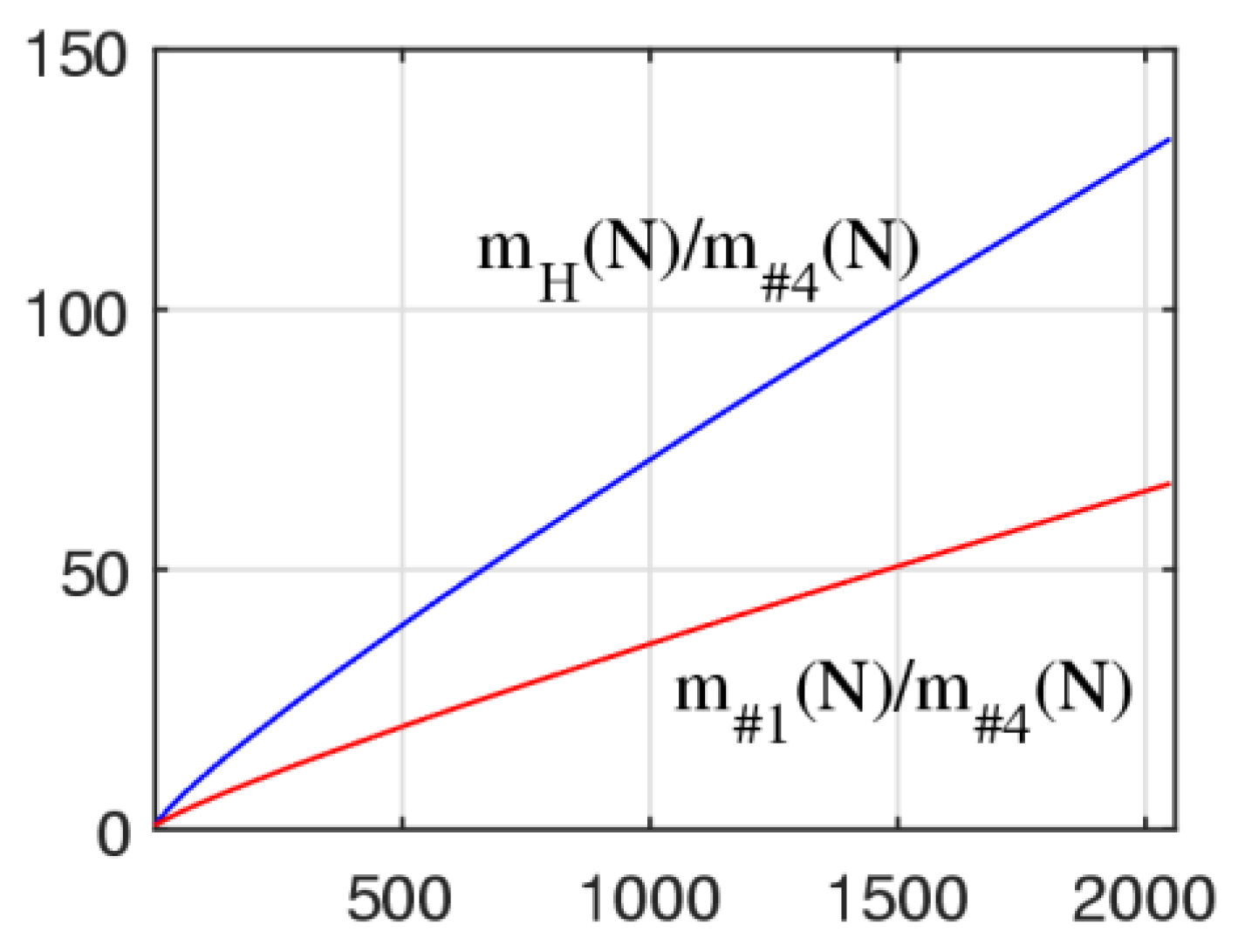
For comparison with the method of DsiHT with path #4, Figure 10 illustrates the ratios of functions $r_1\left(N\right)=m_H\left(N\right)/m_{\#4}\left(N\right)$ and $r_2\left(N\right)=m_{\#1}\left(N\right)/m_{\#4}\left(N\right)$ in the integer interval [2,2048]. These two curves are approximately equal to the lines with the slops $a_1=m_H\left(2048\right)/m_{\#4}\left(2048\right)\approx 132.77$ and $a_2=m_{\#1}\left(2048\right)/m_{\#4}\left(2048\right)\approx 66.51.$

5. Complex QsiHT

In this section, we describe the complex DsiHT. As shown in [33], there are different complex matrices $2\times 2$that can be used as the basis elements to compose the $N$-point complex DsiHT.

A. First, we consider the following 2×2 matrix:

$$M={\displaystyle \frac{1}{\sqrt{{\left|x\right|}^2+|y{|}^2}}}\left[\begin{array}{rr}\overline{x}& \overline{y}\\ -y{\displaystyle \frac{\overline{x}}{\left|x\right|}}& \left|x\right|\end{array}\right].$$

(48)

Numbers $x_0$ and $x_1$ are complex. The matrix $M$ is unitary and its determinant $\det M=\overline{x}/\left|x\right|$ and $\left|\det M\right|=1.$ The matrix product

$$M\left[\begin{array}{c}x\\ y\end{array}\right]={\displaystyle \frac{1}{\sqrt{{\left|x\right|}^2+|y{|}^2}}}\left[\begin{array}{c}{\left|x\right|}^2+|y{|}^2\\ 0\end{array}\right]=\left[\begin{array}{c}\sqrt{{\left|x\right|}^2+|y{|}^2}\\ 0\end{array}\right].$$

(49)

It should be noted that such matrices are used in quantum computation for realization of complex multi-qubit operations [34]. Therefore, this matrix is decomposed by basic 2$\times$2 operations, or gates. For that, the polar form of the numbers is considered, that is,$x=\left|x\right|e^{i{\phi }_0}$and $y=\left|y\right|e^{i{\phi }_1}$. Then, Equation (48) can be written as

$$M={\displaystyle \frac{1}{\sqrt{{\left|x\right|}^2+|y{|}^2}}}\left[\begin{array}{rr}\left|x\right|e^{-i{\phi }_0}& \left|y\right|e^{-i{\phi }_1}\\ -\left|y\right|e^{i{(\phi }_1-{\phi }_0)}& \left|x\right|\end{array}\right].$$

(50)

This complex matrix can be encoded by four angles in the following way. First, we calculate the angle $\vartheta =-\mathrm{atan}(\left|y\right|/\left|x\right|$) and then denote the cosine and sine coefficients

$$\cos \vartheta ={\displaystyle \frac{\left|x\right|}{\sqrt{{\left|x\right|}^2+|y{|}^2}}}\mathrm{a}\mathrm{n}\mathrm{d}\sin \vartheta =-{\displaystyle \frac{\left|y\right|}{\sqrt{{\left|x\right|}^2+|y{|}^2}}}.$$

(51)

The matrix $M$ can be written as

$$M=\left[\begin{array}{rr}{e}^{-i{\phi }_0}\cos \vartheta & -e^{-i{\phi }_1}\sin \vartheta \\ e^{i{(\phi }_1-{\phi }_0)}\sin \vartheta & \cos \vartheta \end{array}\right]=\left[\begin{array}{rr}1& 0\\ 0& e^{-i{\phi }_0}\end{array}\right]\left[\begin{array}{rr}{e}^{-i{\phi }_0}\cos \vartheta & -e^{-i{\phi }_1}\sin \vartheta \\ e^{i{\phi }_1}\sin \vartheta & e^{i{\phi }_0}\cos \vartheta \end{array}\right],$$

(52)

or

$$M=\left[\begin{array}{rr}1& 0\\ 0& e^{-i{\phi }_0}\end{array}\right]\left[\begin{array}{rr}{e}^{-i{(\phi }_0+{\phi }_1)/2}& 0\\ 0& e^{i{(\phi }_0+{\phi }_1)/2}\end{array}\right]\left[\begin{array}{rr}\cos \vartheta & -\sin \vartheta \\ \sin \vartheta & \cos \vartheta \end{array}\right]\left[\begin{array}{rr}{e}^{-i{(\phi }_0-{\phi }_1)/2}& 0\\ 0& e^{i{(\phi }_0-{\phi }_1)/2}\end{array}\right].$$

(53)

The first matrix in this factorization is known as the phase shift, the 2^nd and 4^th ones are $Z$-rotations [35], and the 3^rd matrix is the matrix of the elementary rotation. Thus, we can encode the matrix $M$ by four angles as $\mathsf{\Phi }=\left\{{\phi }_0,{\phi }_0+{\phi }_1,\vartheta ,{\phi }_0-{\phi }_1\right\}.$ The QR-factorization of a complex matrix by such complex $M$ matrices is described in detail in [34]. For this purpose, the concepts of the complex DsiHT with the strong and weak carriage-wheels are used.

Other 2$\times$2 matrices also can be used, instead of the matrix $M$. We mention the known complex Givens rotation with the matrix [4]

$$G={\displaystyle \frac{1}{\sqrt{{\left|x_0\right|}^2+|x_1{|}^2}}}\left[\begin{array}{cc}{|x}_0|& {\displaystyle \frac{x_0}{{|x}_0|}}{\overline{x}}_1\\ -x_1{\displaystyle \frac{{\overline{x}}_0}{{|x}_0|}}& {|x}_0|\end{array}\right],\det G=1.$$

(54)

When applying the matrix $G$ on the vector-generator ${\left(x_0,x_1\right)}^{\text{'}},$ we obtain $x_0/{|x}_0|\left(\sqrt{{\left|x_0\right|}^2+|x_1{|}^2},0\right)\text{'}$. Two coefficients of this matrix are real, and in the matrix $M$, only one coefficient is real. We can consider the complex matrix with all complex coefficients. For instance, the unitary matrix is defined as

$$T={\displaystyle \frac{\mathrm{s}\mathrm{i}\mathrm{g}\mathrm{n}\left(\mathrm{R}\mathrm{e}\mathrm{a}\mathrm{l}\left(x_0\right)\right)}{\sqrt{{\left|x_0\right|}^2+|x_1{|}^2}}}\left[\begin{array}{rr}{\overline{x}}_0& {\overline{x}}_1\\ -x_1& x_0\end{array}\right],$$

(55)

for which $T(x_0,x_1)\text{'}$= $\mathrm{s}\mathrm{i}\mathrm{g}\mathrm{n}(\mathrm{R}\mathrm{e}\mathrm{a}\mathrm{l}\left(x_0\right)\left(\sqrt{{\left|x_0\right|}^2+|x_1{|}^2},0\right)\text{'}.$ The complex vector $(x_0,x_1)$ is rotated to the positive or negative direction of the real axis. The matrices $G$ and $T$ can be expressed by the matrix $M$ as

$$G=\left[\begin{array}{rr}{\displaystyle \frac{x_0}{{|x}_0|}}& 0\\ 0& 1\end{array}\right]M\mathrm{a}\mathrm{n}\mathrm{d}T=\mathrm{s}\mathrm{i}\mathrm{g}\mathrm{n}(\mathrm{R}\mathrm{e}\mathrm{a}\mathrm{l}\left(x_0\right)\left[\begin{array}{rr}1& 0\\ 0& {\displaystyle \frac{{|x}_0|}{{\overline{x}}_0}}\end{array}\right]M,\mathrm{i}\mathrm{f}{x}_0\ne 0.$$

(56)

The comparison of QR-factorizations of a complex square matrix by the matrices $M$, $G$, and $T$, when using the weak and strong DsiHT, is given in [33] together with examples and MATLAB-based codes.

The following should be noted about the matrix $M$. The QR-factorization by this matrix can be calculated analytically without rotation angles and matrices [32]. For simplicity of calculations, we consider the weak DsiHT. First, let the matrix $A$ be real. The following notations for an input $N$-dimensional vector $\mathit{z}$ and the vector generator $\mathit{x}$ are used:

$$E_n\left(\mathit{z},\mathit{x}\right)=z_0{x}_0+z_1{x}_1+\dots +z_{n-1}{x}_{n-1},n=1:N$$

(57)

and

$${\left[E_n\left(\mathit{x}\right)\right]}^2=E_n\left(\mathit{x},\mathit{x}\right)=x_0^2+x_1^2+\dots +x_{n-1}^2,$$

(58)

for the partial energies $E_n\left(\mathit{x}\right)$ of the signal generator. The DsiHT of the input vector $\mathit{z}=(z_0,z_1,\dots .,z_{N-1})$, that is, $H_{N,\#1}\mathit{z}=(z_0^{\left(N-1\right)},z_1^{\left(1\right)},z_2^{\left(1\right)}\dots ,z_{N-1}^{\left(1\right)})$ can be calculated by the correlation data, as follows:

$$z_0^{(N-1)}=E_N\left(\mathit{z},\mathit{x}\right)/E_N\left(\mathit{x}\right),$$

(59)

$$z_n^{\left(1\right)}={\displaystyle \frac{E_n\left(\mathit{x},\mathit{x}\right)z_n-E_n\left(\mathit{z},\mathit{x}\right)x_n}{E_{n+1}\left(\mathit{x}\right)E_n\left(\mathit{x}\right)}},n=1:\left(N-1\right).$$

(60)

For a given generator $\mathit{x}$, all values of $E_n\left(\mathit{x},\mathit{x}\right)$ and $E_{n-1}\left(\mathit{x}\right)E_n\left(\mathit{x}\right),$ can be calculated in advance. The coefficients $h_{n,m},n,m=0:\left(N-1\right),$of the matrix $H_{N,\#1}$ can be obtained from Equations (57)–(60). For that, the standard procedure is used. The m-th column of this matrix is the DsiHT of the unit vector ${\mathit{e}}_m=(0,0,...,1,...0)\text{'}$, with 1 on the m-th position. Therefore, all coefficients can be calculated using the formulas

$$h_{0,m}={\displaystyle \frac{E_N\left({\mathit{e}}_m,\mathit{x}\right)}{E_N\left(\mathit{x}\right)}},h_{n,m}={\displaystyle \frac{{\left[E_n\left(\mathit{x}\right)\right]}^2{{(\mathit{e}}_m)}_n-E_n\left({\mathit{e}}_m,x\right)x_n}{E_{n+1}\left(\mathit{x}\right)E_n\left(\mathit{x}\right)}},n=1:\left(N-1\right).$$

(61)

The diagonal coefficients of this matrix $h_{n,n}=E_n\left(\mathit{x}\right)/E_{n+1}\left(\mathit{x}\right)$ represent the ratios of the energies of the first n components of the signal to the $(n+1)$ components.

When the matrix $A$ is complex, the complex DsiHT can be calculated by using the similar formulas. The partial cross-correlations of the complex input $\mathit{z}$ with the complex generator $\mathit{x}$ are calculated by

$$E_n\left(\mathit{z},\mathit{x}\right)=z_0{\overline{x}}_0+z_1{\overline{x}}_1+\dots +z_{n-1}{\overline{x}}_{n-1},n=1:N$$

(62)

and the partial energies $E_n\left(\mathit{x}\right)$ of the generator are calculated by

$${\left[E_n\left(\mathit{x}\right)\right]}^2=E_n\left(\mathit{x},\mathit{x}\right)={\left|x_0\right|}^2+{\left|x_1\right|}^2+\dots +{\left|x_{n-1}\right|}^2.$$

(63)

The above matrices $M$, $G$, and $T$ can be used for calculating the DsiHTs with fast paths #3 and #4. However, we consider another and more effective way to perform the basic operation $\left(x,y\right)\to (z,0)$ on complex data.

B. We introduce a new matrix instead of the above matrix $M$. First, we remove the phases from the complex numbers $x$ and $y$, as $\left(x,y\right)\to \left(\left|x\right|,\left|y\right|\right).$ In the matrix form, this operation can be written as

$$\left[\begin{array}{rr}{e}^{-i{\phi }_0}& 0\\ 0& e^{-i{\phi }_1}\end{array}\right]\left[\begin{array}{c}x\\ y\end{array}\right]=\left[\begin{array}{rr}{e}^{-i{\phi }_0}& 0\\ 0& 1\end{array}\right]\left[\begin{array}{rr}1& 0\\ 0& e^{-i{\phi }_1}\end{array}\right]\left[\begin{array}{c}x\\ y\end{array}\right]=\left[\begin{array}{c}\left|x\right|\\ \left|y\right|\end{array}\right].$$

(64)

Then, the elementary rotation can be used on the real vector,

$$T\left[\begin{array}{c}\left|x\right|\\ \left|y\right|\end{array}\right]=\left[\begin{array}{cc}\cos \vartheta & -\sin \vartheta \\ \sin \vartheta & \cos \vartheta \end{array}\right]\left[\begin{array}{c}\left|x\right|\\ \left|y\right|\end{array}\right]=\left[\begin{array}{c}\sqrt{{\left|x\right|}^2+{\left|y\right|}^2}\\ 0\end{array}\right].$$

(65)

Here, the rotation angle is calculated as $\vartheta =-\arctan \left(\left|y\right|/\left|x\right|\right)$. If $x=0$, then $\vartheta =-\pi /2$. We obtain the following complex-to-real transformation:

$$A:\left(\mathit{x},\mathit{y}\right)\to \left(\sqrt{{\left|x\right|}^2+{\left|y\right|}^2},0\right),$$

(66)

with the matrix

$$A=\left[\begin{array}{cc}\cos \vartheta & -\sin \vartheta \\ \sin \vartheta & \cos \vartheta \end{array}\right]\left[\begin{array}{rr}{e}^{-i{\phi }_0}& 0\\ 0& e^{-i{\phi }_1}\end{array}\right].$$

(67)

This matrix is simple when compared to the matrix $M$ and it can be encoded by three angles $\mathsf{\Psi }=\left\{{\phi }_0,{\phi }_1,\vartheta \right\}.$ We also can write ${A=A(\phi }_0,{\phi }_1,\vartheta )$. If the input $x$ and $y$ are real, we prefer to use the original matrix of rotation, which is defined in Equation (1). Then, the matrix will be encoded as $\mathsf{\Psi }=\left\{0,0,\vartheta \right\}$.

Example 3.

Let us consider the complex 5-point signal

$$\mathit{x}=(x_0,x_1,x_2,x_3,x_4)=\left(1+i,-2+3i,5+4i,3+i,4-2i\right),‖\mathit{x}‖=\sqrt{86}.$$

(68)

The matrix of the 5-point DsiHT degenerated by $\mathit{x}$ and path #4 has the following complex unitary $4\times 4$ matrix:

$$H_5=\left[\begin{array}{ccccc}0.1078& -0.2157& 0.5392& 0.3235& 0.4313\\ -0.0652& -0.3569& -0.3258& 0.5354& -0.2606\\ -0.1720& 0& 0.4614& 0& -0.6880\\ 0& 0.3658& 0& 0.7132& 0\\ -0.6742& 0& 0& 0& 0.2697\end{array}\right]$$

(69)

This matrix has eight zero coefficients, as in the case of real matrices. The determinant of the matrix is equal to $\det A=-0.9443+0.3292i$ and $|\det H|=1.$ Up to the constant $0.1078=1/\sqrt{86}$, the first row of the matrix is the generator $\mathit{x}$, that is, it is equal to $\mathit{x}/‖\mathit{x}‖.$ The diagram of this transformation is shown in Figure 11 and it looks like what is shown in Figure 7 in part (b). Only, the butterflies with rotations $T_k,k=1:4,$ are changed by the complex operations $A_k={A(\phi }_{0;k},{\phi }_{1;k},{\vartheta }_k)$.

All angles of the complex operations $A_k,k=1:4,$ in this DsiHT are given in Table 7.

Now, we consider the example of the QR-factorization of a complex matrix by the DsiHT with path #4.

Example 4.

Consider the following 5$\times$5 complex matrix:

$$A=\left[\begin{array}{rrrrr}4& 3& 1& 5& -6\\ 8& 1& -3& 5& 9\\ -7& 6& 2& 8& 3\\ 9& 8& 3& -5& 7\\ 5& 4& -2& 9& 3\end{array}\right]+i\left[\begin{array}{rrrrr}-1& 1& 3& 5& 4\\ 3& 5& -1& 1& -1\\ 2& 3& 4& -2& 4\\ -2& 2& 3& -2& -1\\ -2& -1& 5& -1& 5\end{array}\right],|\det A|>117710.$$

(70)

The QR-factorization of this matrix, ${{{H_{2}H}_{3}H}_{4}H}_5:A\to R,$ by four complex DsiHTs each with path #4, results in the following matrices:

$$\begin{gathered} Q_H=Q_{H;\#4}=\left[\begin{array}{rrrrr}0.2495& 0.1281& 0.1843& 0.2960& 0.1733\\ 0.4990& -0.1047& -0.0140& 0.4973& -0.5008\\ -0.4366& 0.7785& 0.0203& 0.1934& -0.2135\\ 0.5614& 0.4034& 0.4464& -0.3933& 0.0999\\ 0.3119& 0.1699& -0.4737& 0.2512& -0.0346\end{array}\right] \\ +i\left[\begin{array}{rrrrr}-0.0624& 0.0528& 0.2389& 0.5986& 0.5896\\ 0.1871& 0.2200& -0.3370& -0.2036& 0.0567\\ 0.1248& 0.3216& -0.0005& -0.0175& -0.0227\\ -0.1248& 0.0891& -0.1497& 0.0693& -0.3277\\ -0.1248& -0.1109& 0.5905& 0.0709& -0.4512\end{array}\right] \end{gathered}$$

(71)

and (upper triangular)

$$\begin{gathered} R_H=R_{H;\#4}=\left[\begin{array}{rrrrr}16.0312& 5.4893& -1.9337& 0.2495& 6.1131\\ 0& 11.2651& 3.8074& 5.6319& 4.5929\\ 0& 0& 6.1090& -4.9145& 4.9253\\ 0& 0& 0& 12.3561& 4.0932\\ 0& 0& 0& 0& -5.3096\end{array}\right] \\ +i\left[\begin{array}{ccccc}0& 2.9942& 2.2456& 0.0624& -1.4347\\ 0& 0& 5.1383& -4.4913& 1.2587\\ 0& 0& 0& -5.1204& 1.7614\\ 0& 0& 0& 0& 7.8876\\ 0& 0& 0& 0& 6.8097\end{array}\right]. \end{gathered}$$

(72)

We need to mention that the coefficients in the diagonal of the upper triangular matrix $R_H$ are real, except the last coefficient. Therefore, the imaginary part of the matrix has four more zeros than the real part. The angles of all ten complex operations $A_k$ in this QR-factorization are given in Table 8.

The unitary matrix is equal to $Q_H=\left({{{H_{2}H}_{3}H}_{4}H}_5\right)\text{'}$. Table 7 can be considered as an encoded table of angles for $Q_H$. Any such encoded table, namely the set of 30 angles, can be used to generate a complex unitary 5$\times$5 matrix. In the general case of $N>2$, such encoded tables of angles for $(N-1)$ DsiHTs with path #4 can be used to generate a complex unitary $N\times N$ matrix. The number of angles in the encoded table is equal to $3/2N\left(N-1\right).$

Now, we analyze the MATLAB version of QR-factorization of the same matrix, $A=Q_M{R}_M$, which is calculated by the function ‘qr.m,’ as ‘[Q_M,R_M]=qr(A).’ The method of the Householder transformations is programmed in this function. Many coefficients of these two matrices are equal up to the sign to the coefficients of the corresponding matrices $Q_H$ and $R_H$. Therefore, we consider the pointwise ratio of the matrices,

$$Real\left(Q_H\right)./Real\left(Q_M\right)=\left[\begin{array}{rrrrr}-1& 1& -1& 1& 0.3032\\ -1& 1& -1& 1& 1.9027\\ -1& 1& -1& 1& 1.4308\\ -1& 1& -1& 1& -0.5074\\ -1& 1& -1& 1& 0.0918\end{array}\right]$$

(73)

$$Imag\left(Q_H\right)./Imag\left(Q_M\right)=\left[\begin{array}{rrrrr}-1& 1& -1& 1& 2.6100\\ -1& 1& -1& 1& 0.1320\\ -1& 1& -1& 1& -0.1473\\ -1& 1& -1& 1& 1.1690\\ -1& 1& -1& 1& 1.8038\end{array}\right],$$

(74)

and

$$Real\left(R_H\right)./Real\left(R_M\right)=\left[\begin{array}{rrrrr}-1& -1& -1& -1& -1\\ \mathrm{*}& 1& 1& 1& 1\\ \mathrm{*}& \mathrm{*}& -1& -1& -1\\ \mathrm{*}& \mathrm{*}& \mathrm{*}& 1& 1\\ \mathrm{*}& \mathrm{*}& \mathrm{*}& \mathrm{*}& 0.6149\end{array}\right],$$

(75)

$$Imag\left(R_H\right)./Imag\left(R_M\right)=\left[\begin{array}{rrrrr}\mathrm{*}& -1& -1& -1& -1\\ \mathrm{*}& \mathrm{*}& 1& 1& 1\\ \mathrm{*}& \mathrm{*}& \mathrm{*}& -1& -1\\ \mathrm{*}& \mathrm{*}& \mathrm{*}& \mathrm{*}& 1\\ \mathrm{*}& \mathrm{*}& \mathrm{*}& \mathrm{*}& 6.8097/0\end{array}\right].$$

(76)

Here, the symbol ‘*’ is used at points where the coefficients of the matrices are zero (as 0/0). The last coefficients of the triangular matrices $R_H\left(\mathrm{5,5}\right)=-5.3096+6.8097i$ and $R_M\left(\mathrm{5,5}\right)=-8.6350.$ The major difference of these matrices is in the coefficients of the last columns.

Although we are writing $A=Q_H{R}_H$ and $A=Q_M{R}_M$, there are small errors in calculation of the matrix $A$ by $Q$ and $R$ matrices. To compare the results of the QR-factorization, the precision of computation has been estimated by the 2-norms of the matrix${∆}_H=(A-Q_H{R}_H)$ and matrix ${∆}_M=(A-Q_M{R}_M)$, by using the MATLAB function “norm.m.” The results of the calculation are

$$‖{∆}_M‖=1.3688\times {10}^{-14},‖{∆}_H‖=0.4956\times {10}^{-14},\mathrm{a}\mathrm{n}\mathrm{d}‖{∆}_M‖/‖{∆}_H‖=2.7621.$$

(77)

Relative to the 2-norm, the error of the QR-factorization by the DsiHTs with fast path #4 is more than two times less than the error when using the method of the Householder transformations.

As mentioned above, the fast paths, like paths #3 and #4, allow us to decompose the matrix $A$ by using matrices with more zero coefficients than when using the paths #1 and #2. It means that less operations of multiplication and addition will be used, and results will be more accurate. That can be verified in this example as well. For instance, we consider the QR-factorization by DsiHTs with path #1 (that is, the DsiHTs with the weak wheel-carriage). The calculations by the analytical Equation (56) result in the following complex matrices:

$$Q_{H;\#1}=\left[\begin{array}{rrrrr}°& °& °& °& -0.6012\\ °& °& °& °& -0.0183\\ °& °& °& °& 0.0390\\ °& °& °& °& 0.3191\\ °& °& °& °& 0.4525\end{array}\right]+i\left[\begin{array}{rrrrr}°& °& °& °& 0.1277\\ °& °& °& °& -0.5037\\ °& °& °& °& -0.2111\\ °& °& °& °& 0.1247\\ °& °& °& °& 0\end{array}\right],$$

(78)

$$R_{H;\#1}=\left[\begin{array}{rrrrr}0& °& °& °& °\\ 0& °& °& °& °\\ 0& 0& °& °& °\\ 0& 0& 0& °& °\\ 0& 0& 0& 0& 7.1959\end{array}\right]+i\left[\begin{array}{rrrrr}0& °& °& °& °\\ 0& 0& °& °& °\\ 0& 0& 0& °& °\\ 0& 0& 0& 0& °\\ 0& 0& 0& 0& 4.7732\end{array}\right].$$

(79)

Here, only those coefficients in the matrices $Q_{H;\#1}$ and $R_{H;\#1}$ are given that differ from the coefficients of the corresponding matrices $Q_{H;\#4}$ and $R_{H;\#4}$. All other coefficients are equal and marked by ‘$°$.’ Note that all coefficients in the above matrices are given with an accuracy of up to 4 decimal places.

The results of the calculation of the 2-norm o the matrix ${∆}_{H;\#1}=A-Q_{H;\#1}{R}_{H;\#1}$ are the following:

$$‖{∆}_{H;\#1}‖=1.1803\times {10}^{-14},‖{∆}_M‖/‖{∆}_{H;\#1}‖=1.1597.$$

(80)

Relative to the 2-norm, the error of the QR-factorization by the DsiHTs with fast path #1 is smaller than the error when using the Householder transformations. However, this 2-norm is larger than the 2-norm $‖{∆}_{H;\#4}‖$ of the factorization by the fast paths. Namely, $‖{∆}_{H;\#1}‖/‖{∆}_{H;\#4}‖=2.3816.$In conclusion, we consider the example of a complex matrix of a large size, and we compare the results of the QR-factorization by the DsiHTs with path #4 with the MATLAB version of the factorization.

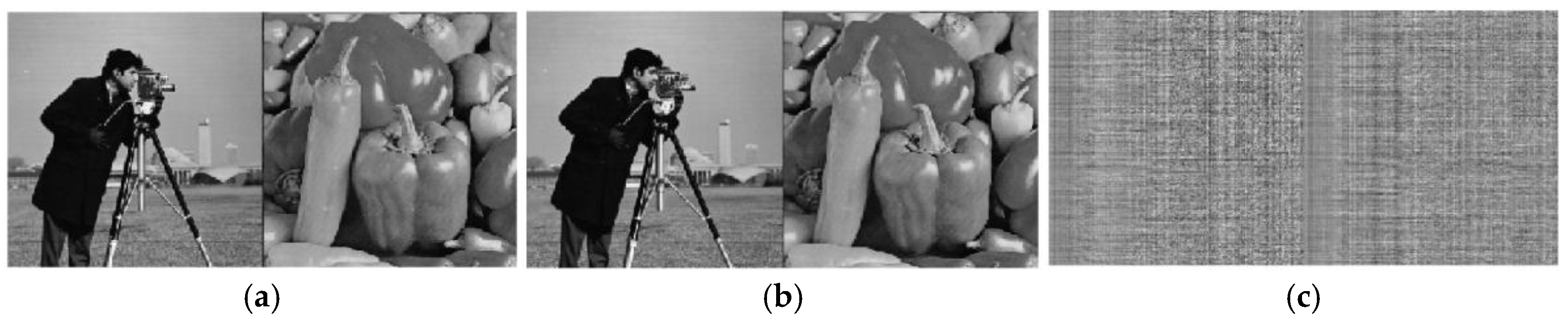
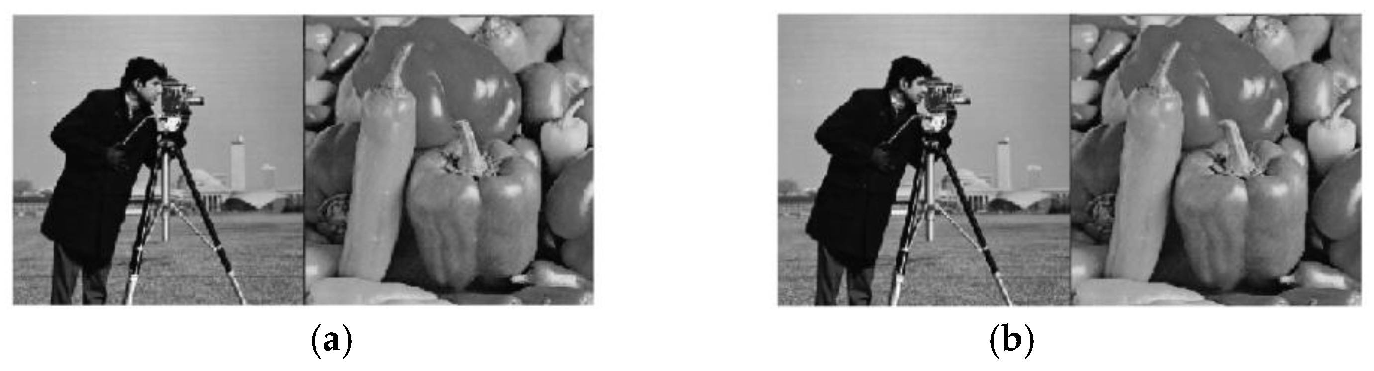
Example 5.

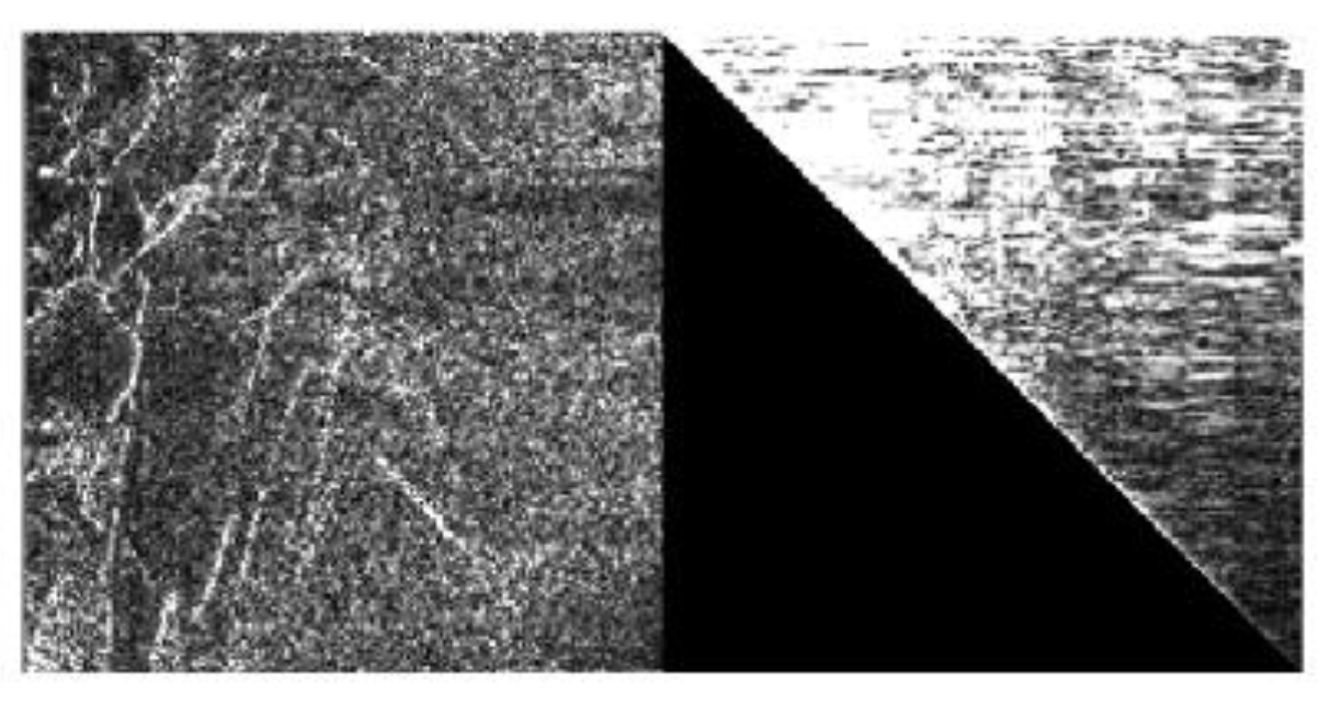
The 256$\times$256 complex matrix $A$ is composed by two real images, as shown in Figure 12 part (a).The real part of this matrix is the ‘cameramen.tif’ image of 256$\times$256 pixels. The imaginary part of this matrix represents the grayscale ‘peppers.tiff’ image of 512$\times 512$ pixels after down-sampling to the size of 256$\times$256 pixels. The real and imaginary parts of this complex matrix are integer-valued non-negative matrices. The result of the DsiHT based QR-factorization of this 256$\times$256 complex image $A$ is shown in part (b). Visually it is difficult to see the difference between these two images in this figure. The difference matrix ${∆}_H$ has values in the small interval ${10}^{-12}\times \left[-\mathrm{0.7105,0.5684}\right]$and is shown in part (c) as the image after scaling, by using the MATLAB function ‘imagesc.m.’ The 2-norm of the difference matrix ${∆}_H=(A-Q_H{R}_H)$ is equal to $‖{∆}_H‖\approx 0.2054\times {10}^{-10}.$

Figure 13 shows the image of the unitary matrix $Q_H$ together with the image of the triangular matrix $R_H$. Since the value of the matrix $Q_H$ are small, this matrix is displayed in an absolute scale with the factor of 2000. The matrix of $R_H$ is also displayed in the absolute scale with the factor of 3.

For comparison, Figure 14 shows the result $Q_M{R}_M$ obtained when using MATLAB code ‘qr(A).’ The 2-norm of the difference matrix ${∆}_M=(A-Q_M{R}_M)$ is equal to $‖{∆}_M‖\approx 0.25344\times {10}^{-10}.$ This 2-norm is 1.2337 times larger than the 2-norm $‖{∆}_H‖.$ Since the original images are integer-valued, the results $Q_H{R}_H$ and $Q_M{R}_M$ can be rounded before displaying them. The rounding of the matrix $Q_M{R}_M$ is shown in Figure 14 in part (b). There is a zero error between the rounded matrix $Q_H{R}_H$ and the matrix $A$. The same is true for the rounded matrix $Q_M{R}_M$.

6. Conclusions

The discrete signal-induced heap transform-based method of the QR-factorization of a square matrix has different realizations. This is explained by the presence of different paths when performing the DsiHTs. Our goal is to show the fast paths which lead to effective calculation of the QR-factorization. The real and complex matrices are considered. Examples of the QR-factorization are given and described in detail for the 4×4, 5×5, and 8×8 real and complex matrices and compared with the Householder transform-based QR-factorization, which is used in MATLAB. The illustrative example with a complex matrix of size 256$\times$256 is also given. Different paths of the DsiHTs were considered together with the traditional path, which we call path #1. The special attention is given to the fast paths, namely path #4. Probably it is the one of fast paths that allow to have the sparsest matrices of the DsiHTs in the QR-factorization and therefore to reduce the number of operations in calculations. We also assume that for complex matrices, the 2$\times$2 matrix described in Equation (67), is the simplest matrix (the complex matrix of rotations) that can be used for effective calculation of the QR-factorization.