
Submitted:
16 December 2025
Posted:
17 December 2025
You are already at the latest version
Abstract
The rapid development of the low-altitude economy is driving significant societal and industrial transformation. Unmanned aerial vehicles (UAVs), as key enablers of this emerging domain, offer substantial benefits in many applications. However, their unauthorized or malicious use poses serious security, safety, and privacy risks, underscoring the critical need for reliable UAV detection technologies. Among existing approaches, such as radar, acoustic, and vision-based methods, radio frequency (RF)-based UAV detection has gained prominence due to its long detection range, robustness to lighting and weather conditions, and capability to identify RF-emitting UAVs even when visually obscured. Nevertheless, conventional RF-based approaches often suffer from limited feature representation and poor generalization. In the past few years, convolutional neural networks (CNNs) have become the mainstream solution for RF signal recognition. However, most real-valued CNNs (RV-CNNs) process only the magnitude component of RF signals, discarding the phase information that carries valuable discriminative characteristics, which may degrade recognition performance. To address this limitation, this paper proposes a complex-valued CNN (CV-CNN) for UAV RF signal recognition, which exploits the full complex-domain structure of RF signals to enhance recognition accuracy and robustness. The proposed CV-CNN accounts for both the magnitude and phase components of RF signals from UAVs, thereby enabling true complex-valued convolutional operations without loss of phase information. The effectiveness of this approach is validated on the DroneRFa dataset, which encompasses RF signals from 25 distinct UAV categories. The impact of model hyperparameters, including network depth, convolutional kernel size, and dropout strategy on recognition performance is investigated through a series of ablation experiments. Comparisons are also conducted between the performance of CV-CNN with identical parameters and RV-CNN, both in noise-free and noisy conditions. The experimental results demonstrate that the CV-CNN exhibits superior robustness and interference resistance in comparison to its real-valued counterpart, maintaining high recognition accuracy even under low signal-to-noise ratio (SNR) conditions.
Keywords:
low-altitude economy
; unmanned aerial vehicle
; radio frequency
; complex-valued convolutional neural network
; ablation experiments
1. Introduction
In recent years, the rapid development of the low-altitude economy has emerged as a powerful driver of societal and industrial advancement [1]. At the heart of this transformation lies unmanned aerial vehicle (UAV) technology, whose rapid advancements have led to a proliferation of applications in both civilian and military domains, garnering considerable attention from academic and industrial communities [2]. UAVs have become a vital technological tool across a wide range of sectors, owing to their high energy efficiency, environmentally benign profile, economically viable operational costs, and superior endurance capabilities [3,4,5]. In practical applications, UAVs are extensively employed for monitoring and surveillance [6], urban traffic monitoring [7], military reconnaissance [8], etc. [9,10,11,12,13,14,15,16,17,18].
Nevertheless, the dissemination and utilization of UAV technology have concomitantly engendered a plethora of technical and security challenges [19]. As demonstrated by a substantial body of research, UAVs have the potential to compromise multiple facets of public safety, privacy protection and social order. Such risks include, but are not limited to, the potential for espionage [20,21], transportation of hazardous materials [22], disruption of power and communication facilities [23], etc. [24,25,26]. This emerging trend signifies a novel method of operation for low-altitude security violations and terrorist activities, thereby posing a significant challenge due to their stealthy nature and the difficulty of their prevention [27,28].
The current absence of a comprehensive regulatory framework for UAVs has given rise to a series of technical vulnerabilities, security risks, threats to public safety and concerns regarding personal privacy breaches [29]. These challenges, whilst catalysing innovation across multiple industries, underscore the urgent necessity for the establishment of robust regulatory frameworks to ensure the safe integration of UAVs into our increasingly technologically interconnected world. The misuse of UAVs for illicit activities poses a significant threat to critical infrastructure and may also disrupt normal societal activities such as civil aviation. This underscores the urgent need to strengthen regulatory frameworks and technological safeguards.
In the context of the proliferation of UAVs and their pervasive utilization, the detection and recognition of UAVs has emerged as a pivotal concern for ensuring low-altitude safety. As demonstrated in the extant literature, research has been conducted on the utilization of acoustic sensors [30] and visual sensors [31] for the detection and recognition of UAVs. However, both types of sensors have very limited detection ranges. Acoustic sensors are highly susceptible to ambient noise, whilst visual sensors are weather-dependent. Radar offers a comparatively longer detection range and performs equally well under all weather conditions. However, the system is susceptible to interference from obstacles and is costly to implement and maintain. As outlined in [32], the employment of RF signals for the recognition of UAVs can effectively circumvent the limitations of the aforementioned three approaches.
The efficacy of deep learning and machine learning in the field of UAV detection has been well-documented in [33,34,35]. CNNs or their variants have achieved notable success in the domain of UAV RF signal recognition tasks [36,37,38,39,40]. However, the majority of contemporary advanced researches employ solely the amplitude component of the UAV RF signal’s complex spectrogram for detection [41,42], frequently disregarding the phase component. The aforementioned studies have typically failed to fully exploit the potential of this complex representation, either neglecting the imaginary part or merely utilizing the magnitude of the complex modulus as an amplitude feature. Such an approach has the potential to compromise the integrity of signal features, thereby reducing the recognition capability of UAV RF signals. RV-CNNs have been observed to encounter difficulties in differentiating between signals with similar amplitudes but significantly different phases. This phenomenon can compromise the model’s resilience to interference [43]. The RF data from UAVs inherently exists in complex form, phase information contains substantial critical features related to device hardware characteristics, such as clock offset and oscillator non-linearity, which can effectively complement amplitude information, thereby enhancing the accuracy of UAV detection and recognition [44]. The significance of phase information is supported by both biological and signal processing fields. As demonstrated in [45], by leveraging phase-encoded data embedded within images, effective retrieval of amplitude-encoded information is facilitated. This is due to the phase process’s capacity to capture salient visual attributes, including edges, shapes, and their respective orientations.
In view of the statistical correlation that characteristically exists between the real and imaginary parts of complex numbers, the utilization of complex-valued modeling approaches is more substantiated. Complex-valued systems impose stronger mathematical constraints than real-valued systems, thereby facilitating the extraction of more intrinsic feature representations [46]. Despite the existence of studies that propose the decomposition of complex values into two real components for the purpose of separate processing, the supposition that a CV-CNN is equivalent to a two-dimensional RV-CNN is erroneous. Research [47] demonstrated that the computational constraints introduced by complex multiplication limit the freedom of CV-CNNs in synaptic weighting, resulting in a fundamental difference in representational capability compared to RV-CNNs.
The employment of CV-CNN ensures the preservation of the algebraic structure inherent within complex data, thus indicating its potential for facilitating the acquisition of more sophisticated feature representations. Extensive research indicates that CV-CNN [48] outperforms traditional RV-CNN [49,50,51,52] across multiple tasks. However, its adoption remains limited, partly due to the maturity of complex-valued convolutional techniques lagging behind real-valued methods [53]. In recent years, the feasibility of constructing and training CV-CNN has been significantly enhanced by mainstream frameworks such as PyTorch, which have begun to support complex-valued convolutional operations [54]. On that basis, this study proposed a CV-CNN model for recognizing UAV RF signal.
The main work and contributions of this paper are concluded as follows.
(1) The establishment of a CV-CNN model has enabled the recognition of RF signals belonging to 25 distinct categories of UAVs. As delineated within the model, the presence of complex convolutional layers, complex batch normalization (CBN) layers, and complex rectified linear unit (CReLU) functions is defined. The real-real, real-imaginary, imaginary-real and imaginary-imaginary components are computed by four independent convolutional kernels, respectively. This satisfies the complex multiplication rule: (a+bi) (c+di) = (ac-bd) + i (ad + bc), thus achieving genuine complex convolutional operations.
(2) The proposed CV-CNN model is validated and evaluated on the preprocessed DroneRFa dataset [55]. A series of ablation experiments are conducted in order to investigate the impact of network depth, kernel size, and dropout mode on model performance.
(3) A comparison is drawn between the performance of CV-CNN and RV-CNN models, which are configured to have identical parameters, in both noise-free and noisy conditions. In light of the rapid advancements being made in the field of UAV technology, coupled with the increasing prevalence of these devices, there is an urgent need to develop intelligent models capable of performing automated or semi-automated RF signal recognition of UAV. This study demonstrates that the employment of the proposed CV-CNN model significantly improves the accuracy of RF signal recognition of UAV under low SNR conditions.
The remainder of this paper is organized as follows. Section 2 introduces the system model. Section 3 provides a detailed description of the proposed CV-CNN model. In Section 4, experimental method and configuration are introduced, results and analysis from evaluations of the proposed CV-CNN model on the DroneRFa dataset are discussed. Finally, we conclude our work in Section 5.
2. System Model
The proposed system model, as shown in Figure 1, is intended to address the classification of RF signals from UAVs, with the objective of achieving this aim through the implementation of a three-stage processing framework. The initial Section 2.1 provides an exposition of signal preprocessing and time-frequency analysis. The subsequent Section 2.2 introduces complex-valued feature extraction methods. Finally, Section 2.3 details the classification and decision process.
2.1. Signal Preprocessing and Time-Frequency Analysis
The input data comprises dual-channel raw RF data stored in .mat files. The present dataset comprises the in-phase components (, ) and the quadrature components (, ), with the ’RF0’ channel data originating from the first channel of the RF receiver and the ’RF1’ channel data from the second channel. The letter ’I’ is used to denote the in-phase (I) component value of the baseband signal, while ’Q’ is used to denote the quadrature (Q) component value. The I/Q components are then combined to form the analyzed signal which can be written as
Then the continuous IQ data stream undergoes fixed-length segmentation, with each segment comprising 5 million sample points. This is equivalent to a duration of 50 milliseconds at a sampling rate of 100 MHz, thereby ensuring that the signal data contained within any two segments does not overlap.
Time-frequency analysis is implemented using the short-time Fourier transform (STFT). For each channel’s data, the STFT transform results are computed separately using the following equation
where the STFT results for channels 0 and 1 are denoted by and . The segmented IQ data for channels 0 and 1 is represented by and , respectively. Subsequently, the complex STFT results are converted to logarithmic power spectral density and which can be written as
and the time-frequency transformation operation can be expressed as
2.2. Complex-Valued Feature Construction and Extraction
During the feature construction phase, the raw logarithmic power spectrum is initially treated as the real part, while the Sobel edge detection results from the spectral image are computed as the imaginary part. In the specific implementation, the imaginary part feature is generated by
where and denote the horizontal and vertical convolutional kernels of the Sobel operator, respectively, and ∗ represents the convolutional operation. The complex-valued feature construction operation, designated as , can be defined as
The feature extraction section is comprised of N, where N is an integer no less than 3, cascaded complex convolutional blocks. Each constituent block is comprised of a complex convolutional layer, a CBN layer, and a CReLU activation layer. The number of channels increases according to the pattern , ultimately resulting in the output of feature maps via adaptive average pooling.
CV-CNN performs feature extraction on through genuine complex-number operations, with the complex convolutional operation adhering to the following mathematical definition which is given by
where the real and imaginary parts of the convolutional kernel weights are denoted by and , respectively, while and represent the real and imaginary parts of the input features. CBN of the input features can be defined as
where and represent the mean values, and denote the squares of the standard deviations of the real and imaginary parts, and is the scaling factor.
The activation function adopts the CReLU form, which involves the application of a ReLU nonlinear transformation to the magnitude of complex signals while preserving phase information. This can be expressed as
where denotes the phase angle of a complex signal.
The complete complex feature extraction network may be expressed as over the complex domain .
where the symbol ∘ is used to emphasise the directionality of data flow, ⊗ denotes the stacking of convolutional blocks, and AP represents the pooling method. In the case of , AP denotes maximum pooling; in the case of , AP denotes adaptive average pooling.
2.3. Classification and Output
The classifier employs a fully connected (FC) layer architecture comprising neurons, with Dropout regularization applied at the 512-dimensional hidden layer at a probability . The system’s output layer generates an m-dimensional logits vector Z, corresponding to binary encodings for m distinct UAV types. The classification decision formula may be expressed as
Softmax is selected as the output function, and the final predicted category formula can be defined as
The complete processing chain may be summarised as follows: The raw IQ signal is subjected to STFT analysis, after which complex features are constructed and extracted. These are then fed into a CV-CNN for classification.
The complete signal processing and classification workflow described by this system may be abstracted as a multi-stage composite function transformation. The mathematical essence of this process is to achieve an end-to-end mapping from raw IQ signals to UAV type identification through a cascade of operations across four stages: time-frequency analysis, complex feature construction, feature extraction, and classification decision-making. The system under discussion can be summarized as formula K which can be written as
The system model’s core innovations can be categorised as follows: The preservation of the phase information of RF signals throughout the process is to be achieved via complex-domain operations. Secondly, the optimisation design of time-frequency analysis and deep learning is to be synergistic. Thirdly, a hybrid feature engineering strategy is to be employed, combining traditional signal processing (Sobel edge detection) with data-driven methods. This structured representation not only reveals the mathematical essence of the system but also highlights its theoretical advantage in achieving high-precision RF signal recognition under complex electromagnetic environments.
3. The Proposed CV-CNN Scheme
CV-CNN is a deep learning architecture that has been specifically designed for the purpose of processing complex-valued data. The present study has demonstrated that the technology under discussion finds extensive applications in fields requiring phase information preservation. Such fields include radar signal processing, medical imaging (e.g. MRI) and wireless communications. The proposed CV-CNN is principally comprised of a feature extraction module and a classifier module. In comparison to conventional RV-CNN, CV-CNN meticulously adheres to intricate mathematical principles in pivotal operations, thereby ensuring the model’s capacity to efficiently discern the magnitude and phase characteristics of complex data.
3.1. Architecture
The architecture of CV-CNN proposed in this paper represents an enhancement of the model introduced in [56], with its overall structure illustrated in Figure 2. The network under consideration adopts a modular design, primarily consisting of two major modules: a feature extractor and a classifier. The system has been engineered to facilitate efficient complex signal processing through the implementation of meticulously designed complex operation layers.
Within the architecture of the input layer, the network is configured to receive complex tensors of size [batch size, 2, 384, 288]. The first channel is responsible for storing the real-part information of the original spectrogram, while the second channel is responsible for storing the imaginary-part information processed by Sobel edge detection. This dual-channel representation is capable of preserving the complex nature of the signal, thereby establishing the mathematical foundation for subsequent processing.
The feature extractor module consists of N (set to 3-6) stacked complex convolutional blocks, each comprising four key components: The complex convolutional layer employs a four-branch real convolutional to simulate complex multiplication. The complex arithmetic rule is implemented rigorously through the parallel branches , , , and . This layer is responsible for preserving the spatial dimensions of the feature map through padding operations, whilst only modifying the channel dimension which may be increased to a maximum of 256 to prevent overfitting and computational explosion. The CBN layer, a key component of the model, jointly normalizes the concatenated real and imaginary parts, thereby preserving the consistency of complex feature distributions. The CReLU activation function is an innovative implementation of a nonlinear transformation in the complex domain. It first calculates the magnitude of the complex number and applies the ReLU operation, then reconstructs the complex output by integrating the original phase information. The pooling layer employs a hybrid strategy, whereby the first N-1 layers utilize max pooling to halve the feature map size sequentially, while the final layer switches to adaptive average pooling to ensure the network can process inputs of varying resolutions.
We devised two dropout modes (Standard and Reduced) as regularization strategies. The "Standard" mode employs a strategy of progressively increasing dropout rate, raising the rate by 0.1 for each additional convolutional layer (initialized at 0.3). The “Reduced” mode employs the same increment logic for the first three layers (initialized at 0.2); however, it forcibly disables dropout from the fourth layer onwards. Ablation experiments demonstrated that this design effectively balanced the model’s generalization capability and representational power.
The classifier module consists of three FC layers, the function of which is to flatten the four-dimensional feature tensor [batch, C, H, W] into a two-dimensional matrix [batch, C×H×W]. The initial FC layer compresses the high-dimensional features (e.g., 18432 dimensions) to 1024 dimensions, while the subsequent layer reduces this further to 512 dimensions, ultimately producing 25-dimensional category logits. The implementation of ReLU activation functions and dropout with a 0.5 probability between each FC layer serves to effectively prevent overfitting.
Utilizing a model comprising four convolutional blocks, a kernel size of three, and a dropout pattern of “Reduced” (4L, 3K, Reduced), the model architecture is illustrated in Table 1. The complete forward propagation process demonstrates the dimensional changes in the data: The input complex signal [batch, 2, 384, 288] undergoes processing through four convolutional blocks, transforming into [batch, 256, 6, 6]. Subsequent to unfolding, this yields a feature vector of [batch, 9216], which is progressively compressed through FC layers to produce an output of [batch, 25]. This architecture design is capable of achieving efficient feature extraction and classification of complex signals while maintaining the mathematical completeness of complex operations.
3.2. Feature Extractor
The core components of the feature extractor of the present study comprise complex convolutional layers, CBN layers, CReLU activation functions, and pooling layers, thereby achieving efficient complex signal processing through a modular design.
3.2.1. Complex Convolutional Layer
The core operation of CV-CNN is complex-valued convolution, which is designed to process complex input data. The mathematical foundation of this approach is predicated on the linear separability of complex multiplication, thus exhibiting a fundamental distinction from real-valued convolution, as shown in Table 2.
In the case of an input complex tensor , where B denotes the batch size, represents the real part (channel 0) and the imaginary part (channel 1), and H and W denote the input height and width, respectively, the tensor can be expressed in this form. It can be demonstrated that, for the complex input and the convolutional kernel , the output can be expressed as
In this context, the symbol ∗ denotes the standard two-dimensional convolutional operation, with and denoting the convolutional kernel weights for the real and imaginary parts, respectively. In practical implementation, complex-valued convolution is approximated through parallel computation using four real-valued convolutional kernels: denotes the convolution of the real part with the real kernel, denotes the convolution of the real part with the imaginary kernel, denotes the convolution of the imaginary part with the real kernel, and denotes the convolution of the imaginary part with the imaginary kernel. The final output is obtained through linear combination:
This design explicitly models the cross-coupling between the real and imaginary parts, rendering it suitable for time-frequency analysis (e.g., STFT features) and coherent signal processing.
Complex-valued convolution offers several advantages over its real-valued counterpart. Firstly, it preserves phase information, which in UAV RF signals carries target motion data, enabling effective modeling of phase variations. Secondly, it exhibits frequency-domain filtering characteristics, with complex kernels functioning as frequency-domain filters that better suit time-frequency analysis tasks (such as STFT feature processing) than real-valued convolution. Thirdly, it offers physical interpretability, as complex operations align with signal processing theory (e.g., analytic signals and Hilbert transform).
3.2.2. CBN Layer
The CBN layer performs independent normalization on the real and imaginary parts to ensure training stability. For complex data , the normalization method is defined as
where BN denotes a standard BatchNorm2d, which can be expressed as
This specific implementation method involves the calculation of and separately for the real and imaginary parts. CBN is a method that has been developed to address the issue of internal covariate shifts in complex data. This process prevents optimization difficulties arising from scale differences between real and imaginary components. The primary benefit of this approach is that it stabilizes the distribution of complex features, thereby accelerating the convergence of training. Additionally, it preserves the independence of the real and imaginary components.
3.2.3. CReLU Layer
CReLU is a nonlinear activation function that defines a magnitude activation while preserving the phase in the complex domain. For a complex number , the magnitude and phase can be written as
The application of a standard ReLU to the magnitude yields , which is given by
Finally, z must be reconstructed in order to derive the CReLU formula
CReLU circumvents the phase distortion issues that arise from conventional real-imaginary separation activation mechanisms by introducing a nonlinear transformation in the vicinity of the origin whilst strictly preserving complex phase information.
3.2.4. Complex Pooling Layer
In CV-CNN, the complex pooling operation is of pivotal importance as a module for the reduction of feature dimensionality, primarily employed to decrease the spatial resolution of feature maps while enhancing translation invariance. In light of the properties inherent to complex data, it is imperative that pooling operations process the real part and the imaginary part separately, thereby ensuring the maintenance of mathematical consistency in complex arithmetic. The specific implementations comprise max pooling and adaptive average pooling.
For the set of complex samples within the sliding window (win) , max pooling independently selects the maximum value for both the real and imaginary parts, whereas average pooling calculates the arithmetic mean. Max pooling and average pooling can be defined as
In the domain of signal processing, the max pooling operation, as a feature dimension reduction method, derives its physical significance primarily from its ability to enhance locally salient features. This approach effectively accentuates locally prominent features exhibiting strong responses, a characteristic of considerable value in UAV RF signal recognition applications. Specifically, within the domain of UAV RF signal processing, this method preserves both the amplitude and phase information of RF signal from the target.
The primary benefit of average pooling is attributable to its capacity for spatial smoothing, a property that is particularly advantageous for the processing of complex signals. The process of averaging serves to effectively suppress random noise in local regions while preserving the overall energy distribution characteristics of the signal. From an implementation perspective, complex average pooling is equivalent to performing standard real-valued average pooling operations separately on the real and imaginary components of the feature map. This approach is not only computationally efficient but, more importantly, maintains the continuity of phase information in the output. In particular, the phase value of the output feature is defined as the weighted average of all complex sample phases within the specified window. This property makes it particularly suitable for applications that require strict phase consistency, such as coherent signal processing and RF data analysis of UAVs.
3.3. Classifier
The classifier module is composed of a FC layer and an output layer, a design that is imperative for processing complex features. The input to the proposed CV-CNN model is a flattened complex feature vector , composed of the real part and the imaginary part . For instance, if the real and imaginary parts each possess 128 dimensions, the input z will have a dimension of 256. The parameter configuration for this layer is defined by the weight matrix which is a matrix of real numbers with dimensions , and the bias vector , which is a real number with dimensions M. The output dimension is denoted by M.
In the actual implementation process, the real part a and the imaginary part b undergo independent matrix multiplication operations (i.e., and ), with the final results being merged. This design approach of separating computations effectively preserves the physical significance of complex features, including both magnitude and phase information. It is particularly well-suited for processing frequency-domain signals or the output features of complex convolutional layers.
The principal function of the FC layer is to map high-dimensional complex features (such as the output of complex convolutional layers) onto the target dimensional space (such as the number of categories in a classification task) and the separation of the real and imaginary components for computation ensures the physical meaning of the complex features is preserved, thereby providing a suitable feature representation for subsequent classification tasks.
The processing flow of the output layer is comprised of two key steps. Firstly, raw output values are generated through the final FC layer. Here, C denotes the number of categories in the classification task. Secondly, these raw output values are converted into a probability distribution via the Softmax function.
The numerator, of this function denotes the exponential operation applied to the output of the i-th neuron, while the denominator sums the exponential scores across all classes, ensuring the normalization property of the probability distribution . Physically interpreted, represents the predicted probability that the input sample belongs to class i.
In practical programming, numerical overflow in exponential operations (such as ) can be avoided by employing the following equivalent form
This logarithmic probability form is not only fully compatible with the cross-entropy loss function but also exhibits superior numerical stability during gradient computation. The core function of the Softmax operator lies in transforming the raw output values by neural networks into probability distributions, thereby providing probabilistic grounds for multiclass classification tasks. As an optimized implementation, Log-Softmax effectively resolves potential issues inherent in numerical computations.
3.4. Loss Function and Backpropagation
During the training process of the CV-CNN model, the design and optimization of the loss function are critical to achieving model convergence. The present study employs the cross-entropy loss function as the optimization objective, the mathematical expression of which can be written as
where denotes the one-hot encoded vector of the true label. This loss function provides explicit guidance for optimizing model parameters by measuring the discrepancy between the predicted distribution and the true distribution.
The proposed CV-CNN model utilizes the Adam optimizer for parameter updates, whose update rules encompass first-order moment estimation , second-order moment estimation , bias correction and parameter update , which can be written respectively as
where denotes the current parameter, represents the current gradient, and is the learning rate. and are set to default values of 0.9 and 0.999, respectively, while is a small constant introduced to ensure numerical stability (default ).
This optimization scheme effectively mitigates gradient oscillation by incorporating first-order and second-order moment estimation; subsequently addresses significant moment estimation bias during the initial phase through a deviation correction mechanism; and finally achieves robust convergence performance across varying parameter dimensions by employing an adaptive learning rate.
During backpropagation, the computation of gradients adheres to the chain rule which is given by
The unique structure exhibited by complex neural networks necessitates the separate computation of gradients, taking into account the real and imaginary components. To elaborate further, the gradient expressions for the weight matrices and can be written as
This decoupled computational approach ensures that complex parameters retain their physical significance throughout the optimization process, while effectively capturing the coupling relationship between the real and imaginary parts.
4. Ablation Experiment
This section conducts ablation experiments on the proposed CV-CNN model under ideal conditions (noise-free) using a spectrogram dataset generated from the raw IQ data within the DroneRFa dataset [55]. The impact of various parameters on the model’s performance in UAV RF signal classification was evaluated using accuracy. In addition, in order to provide a more comprehensive comparison of the performance of CV-CNN with that of traditional RV-CNN models, ablation studies were also conducted on the RV-CNN models. It is noteworthy that both RV-CNN and CV-CNN employed model structures and training logic that were identical throughout the course of the aforementioned ablation experiments.
In consideration of the pervasive presence of noise interference in practical application scenarios, subsequent research in Section 4.2 will undertake a more profound analysis of the performance differences between the two models under varying SNR conditions. This will facilitate a more comprehensive evaluation of the applicability of CV-CNN and RV-CNN for real-world applications.
4.1. Experimental Method
The present study has devised a comprehensive experimental framework for CV-CNN with the objective of identifying RF signals from UAVs, as shown in Figure 3. During the construction and preprocessing of the data set, the DroneRFA data set was used, which comprises IQ data from 25 categories of RF signals from UAVs. The raw IQ data underwent fixed-length segmentation, with each segment containing samples corresponding to a 50ms duration at a 100 MHz sampling rate. The signal data within any two segments did not overlap. Subsequently, each segmented IQ data underwent STFT, with the following parameters being utilized: The 1024-point Hanning window, with a 50% overlap, is utilized in conjunction with a 1024-point FFT operation, ensuring a consistent 100 MHz sampling rate. This process yielded a dataset comprising 38480 spectrograms with a resolution of .
The preprocessing workflow encompasses four critical stages: during spectrogram processing, the raw image () undergoes effective region cropping; for spectrogram visualization, a 60 dB dynamic range is set (referenced to maximum power), employing a Jet color palette, with the frequency axis display range set to MHz to 50 MHz to achieve centered display. Subsequently, a logarithmic transformation enhances the discernibility of low-intensity signal features. The final output comprises a pixel PNG image, which serves as input for the RV-CNN and the real-part channel input for the CV-CNN. Finally, the Sobel edge detection algorithm is applied to the PNG image to generate the imaginary-part channel input, thereby constructing the complete complex representation for the CV-CNN. A comparative analysis is conducted to assess the performance of the two models under both noise-free and noisy conditions.
In terms of network architecture design, the proposed CV-CNN model comprises three core components: the complex convolutional layer strictly adheres to complex multiplication rules to ensure mathematical completeness of complex operations; the CBN layer performs independent normalization on the real and imaginary parts to maintain feature numerical stability; and the CReLU activation function implements nonlinear transformation based on complex magnitude while preserving phase information. Specifically, the network employs a dynamic feature extractor design that allows flexible adjustment of network depth based on the parameters of the ablation experiment.
The design of the ablation experiment employs a full-combination scheme of three factors in order to systematically evaluate the impact of different network configurations on performance. The first factor examines the influence of the number of convolutional layers (3, 4, 5, or 6 layers) on feature extraction capability; the second factor compares the local feature capture ability of different convolutional kernel sizes ( and ). The third factor contrasted two Dropout regularization strategies. The "Standard" mode employed a progressively increasing dropout rate (0.3–0.8) across layers, whilst the “Reduced” mode applied a dropout rate increment strategy (0.2–0.4) exclusively to the first three layers. This multi-factor experimental design provides exhaustive empirical evidence for the optimization of model performance.
4.2. Experimental Configuration
For the 25 categories of UAV RF signals, the experiment randomly partitioned the data into training, validation, and test sets at a ratio of . The implementation of the neural network model was accomplished through the utilization of the PyTorch framework on a Ubuntu 22.04.5 platform. The training, validation, and testing phases of the process were conducted on an NVIDIA RTX 3090, utilizing the Adam optimizer and the cross-entropy loss function. The initial learning rate, weight decay, batch size and training epoch were separately set to , , 8 and 50.
4.3. Results and Analysis
4.3.1. Impact of Parameters on CV-CNN
In this section, the impact of network depth, kernel size, and dropout mode on the classification accuracy of the CV-CNN model was evaluated based on the results of the ablation experiments shown in Table 3.
Experimental results indicated that network depth is the most substantial factor influencing the performance of the CV-CNN model. As shown in Figure 4, the performance of the model notably improved with an increase in network depth from 3 to 4 layers. This suggests that an increase in depth effectively enhances the model’s capacity for feature extraction. However, when the depth was increased to five layers, the marginal benefit diminished, with performance even showing slight deterioration. In the (5, 3, Reduced) configuration, the accuracy of the model decreased to 8.52%, which demonstrates the model’s extreme sensitivity to parameter combinations within this range and its susceptibility to training instability. As the depth was increased to six layers, the model demonstrated a significant deterioration in performance, with accuracy falling below 10% in the majority of configurations. This finding suggests that the network has become excessively deep, which has resulted in substantial gradient-related issues or the overfitting of the model. Consequently, subsequent analyses in this section exclude models with a depth of 6 and the (5, 3, Reduced) configuration.
The impact of kernel size on CV-CNN performance is relatively minor, exhibiting no discernible pattern, as illustrated in Figure 5. When the network depth was set at 3, models utilizing convolutional kernels exhibited marginally superior performance in comparison to those employing kernels. At a depth of 4, kernel-based models demonstrated slightly superior performance compared to their counterparts. However, at a depth of 5, the kernel-based models once again exhibited slight superiority over the kernel-based models, suggesting a transition in the relative effectiveness of the two kernels as the network depth increases. This phenomenon suggests that the influence of kernel size may be modulated by interactions with other parameters, rather than being an independent dominant factor.
The impact of dropout mode on model performance is highly correlated with network depth, as shown in Figure 6. When model complexity was moderate (network depth=3, 4), the ’Reduced’ mode often yielded a slight performance improvement, such as an increase from 96.08% for (3, 3, Standard) to 98.35% for (3, 3, Reduced). However, as the complexity of the model increased, the ’Reduced’ mode was shown to significantly exacerbate overfitting due to insufficient regularization strength, leading to a performance collapse. For instance, the configuration (5, 3, Reduced) attained an accuracy of a mere 8.52%.
4.3.2. Comparison of Model Performance in Noise-Free Conditions
This section drew parallels between the performance of CV-CNN and RV-CNN models operating under identical experimental and training protocols in the absence of noise, as illustrated in Table 4.
Comparison of the performance of the two model types reveals that both can achieve near-100% accuracy under optimal configurations (e.g. network depth=4 or 5 in most cases), indicating comparable theoretical upper limits. However, RV-CNN requires lower parameter tuning costs to achieve equivalent performance and demonstrates significant advantages in terms of model stability. As shown in Figure 7, CV-CNN demonstrated variability in performance when the network depth ranged from 3 to 5, while RV-CNN exhibited consistent and superior performance. For instance, under the configuration (5, 3, Reduced), RV-CNN achieved 100% accuracy, whereas CV-CNN registered only 8.52%. Furthermore, RV-CNN demonstrated greater fault tolerance to increased network depth, as shown in Figure 7(b). When the network depth was designated as 6, the performance of CV-CNN was significantly compromised (often falling below 10% accuracy), while RV-CNN exhibited notable resilience with certain configurations. For instance, under (6, 3, Standard) and (6, 5, Standard) configurations, RV-CNN achieved accuracies of 99.98% and 84.13%, respectively.
In conclusion, the RV-CNN models offer enhanced stability and resistance to overfitting, while exhibiting comparable peak performance to the CV-CNN models. This renders the RV-CNN models a more reliable choice.
However, it should be noted that the aforementioned conclusions are obtained under ideal experimental conditions, devoid of noise. In view of the pervasive presence of noise interference in practical application scenarios, we will further analyze the performance differences between the two models under varying SNRs in the subsequent section. This extensive investigation will provide a more comprehensive assessment of the suitability of CV-CNN and RV-CNN for real-world applications.
4.3.3. Comparison of model performance in different SNRs
In this section, a systematic comparison was made between the recognition accuracy of the CV-CNN model and the traditional RV-CNN model under varying SNRs through experimental evaluation. The performance of both models was comprehensively assessed across an SNR range from -20dB to 20dB. As indicated by the findings in Section 4.3.1, both the CV-CNN and RV-CNN models demonstrated substantial degradation when the network depth reached six layers. Consequently, we abandoned analysis of models with a depth of six layers.
The experimental results revealed a conspicuous discrepancy in performance between the two models, particularly in regions characterised by low SNR, as shown in Figure 8. At extremely low SNR levels (-20 dB to -10 dB), the two models demonstrated fundamental discrepancies in their performance. As shown in Figure 8(a), all configurations of the CV-CNN model demonstrated substandard performance at -20 dB. However, certain models, including the (5, 5, Standard) and (5, 5, Reduced) models, exhibited foundational classification capabilities, attaining accuracy rates that significantly exceeded random guessing levels. When SNR improved to -10 dB, the CV-CNN models demonstrated substantial performance gains, with most configurations achieving accuracy rates exceeding 80%. When subject to low-SNR conditions that were identical in all respects, failure of the RV-CNN models was complete, as shown in Figure 8(b). At both -20 dB and -10 dB, the RV-CNN models demonstrated an accuracy rate of less than 10%, indicating an inability to extract effective features for classification in the presence of strong noise.
Within the SNR range of -10 dB to 0 dB, the CV-CNN demonstrated its most pronounced performance advantage. At an SNR of 0 dB, the CV-CNN approached near-complete convergence. The majority of model configurations achieved accuracy rates in excess of 95%, with configurations such as (5, 5, Standard) and (4, 5, Standard) attaining or approaching 100% accuracy. In contrast, the performance of RV-CNN in this range exhibited a considerable delay. Even at 0 dB, the accuracy of all RV-CNN models remained below 10%, indicating a substantial discrepancy compared to CV-CNN models.
As SNR continued to increase, the performance of the RV-CNN models began to improve rapidly. Beyond an SNR exceeding 10 dB, the accuracy of all CV-CNN and RV-CNN models approached saturation, reaching or approaching the ultimate performance threshold of 100%. This finding indicated that, in conditions of high SNR, both models demonstrate the capacity to leverage the unique signal characteristics in their entirety.
In summary, CV-CNN demonstrated overwhelming superiority over RV-CNN under low SNR conditions. CV-CNN has been shown to maintain effective feature extraction and classification capabilities even in extremely low SNR environments (as low as -20 dB), where RV-CNN has been demonstrated to fail, thus demonstrating the robust noise resilience of CNN-CNN. Concurrently, CV-CNN exhibited a higher performance threshold, achieving near-perfect classification performance at 0 dB SNR, whereas RV-CNN remained virtually inoperable at this SNR level. Due to its intrinsic capacity to completely preserve and process both signal phase and amplitude, CV-CNN possesses distinct advantages in the handling of low-SNR, non-stationary signals. This renders it exceptionally well-suited for tasks involving poor signal quality in practical scenarios such as communications, radar, and RF applications.
In practical applications, when the anticipated SNR in the working environment is below 10dB, the CV-CNN architecture should be prioritised. Conversely, in high SNR environments (more than 10dB), the performance discrepancy between the two models is significantly reduced, enabling selection based on computational efficiency and other factors. The anomalous performance observed at five layers and the comprehensive degradation at six layers provide crucial avenues for future research. This finding necessitates further investigation into the optimal depth constraints for CV-CNN and the underlying mechanisms governing their interaction with regularisation strategies.
5. Conclusion
This study aims to implement CV-CNN in recognizing RF signals from UAVs. In order to leverage phase information, a CV-CNN incorporating complex convolutional layer, CBN, CReLU, complex pooling, and complex backpropagation algorithms is proposed. A series of ablation experiments were conducted on the DroneRFa dataset, with the aim of comparing the performance of the proposed CV-CNN with that of a RV-CNN sharing the same architecture. The experimental results demonstrate that the CV-CNN exhibits superior robustness and interference resistance in comparison to RV-CNN of identical architecture, maintaining high recognition accuracy even under low SNR conditions. This research provides a foundation for the broad application of CV-CNN in the domain of UAV RF signal recognition.
Author Contributions
Conceptualization, Y.X. and J.M.; methodology, J.M. and X.J.; software, Y.X.; validation, Y.X., J.M.; formal analysis, Y.X. and W.L.; investigation, Y.X. and J.M.; resources, Y.X. and W.L.; data curation, Y.X.; writing—original draft preparation, Y.X.; writing—review and editing, Y.X. and J.M.; visualization, Y.X.; supervision, X.J. and W.L.; project administration, Y.X. and J.M. All authors have read and agreed to the published version of the manuscript.
Funding
This research received no external funding.
Institutional Review Board Statement
Not applicable.
Informed Consent Statement
Not applicable.
Data Availability Statement
The original contributions presented in this study are included in the article. Further inquiries can be directed to the corresponding author.
Conflicts of Interest
The authors declare no competing interests.
Abbreviations
The following abbreviations are used in this manuscript:
| UAV | Unmanned aerial vehicle |
| RF | Radio frequency |
| CNN | Convolution neural network |
| CV-CNN | Complex-valued convolution neural network |
| RV-CNN | Complex-valued convolution neural network |
| SNR | Signal-to-noise ratio |
| CBN | Complex batch normalization |
| CReLU | Complex rectified linear unit |
| STFT | Short-time Fourier Transform |
| FC | Fully connected layer |
References
- Cui, Q.; You, X.; Wei, N.; Nan, G.; Zhang, X.; Zhang, J.; Lyu, X.; Ai, M.; Tao, X.; Feng, Z.; et al. Overview of AI and communication for 6G network: fundamentals, challenges, and future research opportunities. Science China Information Sciences 2025, 68, 171301. [Google Scholar] [CrossRef]
- Radoglou-Grammatikis, P.; Sarigiannidis, P.; Lagkas, T.; Moscholios, I. A compilation of UAV applications for precision agriculture. Computer Networks 2020, 172, 107148. [Google Scholar] [CrossRef]
- Kim, S.; Moon, I. Traveling Salesman Problem With a Drone Station. IEEE Transactions on Systems, Man, and Cybernetics 2019, 49, 42–52. [Google Scholar] [CrossRef]
- Jung, S.; Yang, P.; Quek, T.Q.S.; Kim, J.H. Belief Propagation based Scheduling for Energy Efficient Multi-drone Monitoring System. In Proceedings of the 2020 International Conference on Information and Communication Technology Convergence (ICTC), 2020; pp. 261–263. [Google Scholar] [CrossRef]
- Alsamhi, S.H.; Ma, O.U.; Ansari, M.S.; Almalki, F. Survey on Collaborative Smart Drones and Internet of Things for Improving Smartness of Smart Cities. IEEE Access 2019, PP. [Google Scholar] [CrossRef]
- Ding, G.; Wu, Q.; Zhang, L.; Lin, Y.; Yao, Y.D. An Amateur Drone Surveillance System Based on Cognitive Internet of Things. IEEE Communications Magazine 2017, 56. [Google Scholar] [CrossRef]
- Alioua, A.; Djeghri, H.E.; Cherif, M.E.T.; Senouci, S.M.; Sedjlmaci, H. UAVs for Traffic Monitoring: A Sequential Game-based Computation Offloading/Sharing Approach. Computer Networks 2020, 177, 107273. [Google Scholar] [CrossRef]
- Husodo, A.Y.; Jati, G.; Alfiany, N.; Jatmiko, W. Intruder Drone Localization Based on 2D Image and Area Expansion Principle for Supporting Military Defence System. In Proceedings of the 2019 IEEE International Conference on Communication, Networks and Satellite (Comnetsat), 2019. [Google Scholar]
- Vihma, T.; Naakka, T.; Sun, Q.; Nygard, T.; Tjernström, M.; Jonassen, M.; Pirazzini, R.; Brooks, I. Impact of assimilation of radiosonde and UAV observations on numerical weather prediction analyses and forecasts in the Arctic and Antarctic. In Proceedings of the EGU General Assembly Conference Abstracts, 5 2020; p. 21750. [Google Scholar] [CrossRef]
- Akram, T.; Awais, M.; Naqvi, R.; Ahmed, A.; Naeem, M. Multicriteria UAV Base Stations Placement for Disaster Management. IEEE Systems Journal 2020, PP, 1–8. [Google Scholar] [CrossRef]
- Ishigami, M.; Sugiyama, T. A Novel Drone’s Height Control Algorithm for Throughput Optimization in Disaster Resilient Network. IEEE Transactions on Vehicular Technology 2020, 69, 16188–16190. [Google Scholar] [CrossRef]
- Bacco, M.; Berton, A.; Ferro, E.; Gennaro, C.; Gotta, A.; Matteoli, S.; Paonessa, F.; Ruggeri, M.; Virone, G.; Zanella, A. Smart farming: Opportunities, challenges and technology enablers. In Proceedings of the 2018 IoT Vertical and Topical Summit on Agriculture - Tuscany (IOT Tuscany), 2018; pp. 1–6. [Google Scholar] [CrossRef]
- Daftry, S.; Hoppe, C.; Bischof, H. Building with Drones: Accurate 3D Facade Reconstruction using MAVs. IEEE 2015. [Google Scholar]
- Shukla, A.; Xiaoqian, H.; Karki, H. Autonomous tracking and navigation controller for an unmanned aerial vehicle based on visual data for inspection of oil and gas pipelines. IEEE 2017. [Google Scholar]
- BanderAlzahrani; Oubbati, O.S.; Barnawi, A.; Atiquzzaman, M.; Alghazzawi, D. UAV assistance paradigm: State-of-the-art in applications and challenges. Journal of Network and Computer Applications 2020, 166. [Google Scholar]
- Nomikos, N.; Michailidis, E.T.; Trakadas, P.; Vouyioukas, D.; Voliotis, S. A UAV-based moving 5G RAN for massive connectivity of mobile users and IoT devices. Vehicular Communications 2020, 25, 100250. [Google Scholar] [CrossRef]
- Bisio, I.; Garibotto, C.; Lavagetto, F.; Sciarrone, A.; Zappatore, S. Unauthorized Amateur UAV Detection Based on WiFi Statistical Fingerprint Analysis. IEEE Communications Magazine 2018, 56, 106–111. [Google Scholar] [CrossRef]
- Shakhatreh, H.; Sawalmeh, A.H.; Al-Fuqaha, A.; Dou, Z.; Almaita, E.; Khalil, I.; Othman, N.S.; Khreishah, A.; Guizani, M. Unmanned Aerial Vehicles (UAVs): A Survey on Civil Applications and Key Research Challenges. IEEE Access 2019, 7. [Google Scholar] [CrossRef]
- Mu, J.; Zhang, R.; Cui, Y.; Gao, N.; Jing, X. UAV Meets Integrated Sensing and Communication: Challenges and Future Directions. IEEE Communications Magazine 2023, 61, 62–67. [Google Scholar] [CrossRef]
- Shi, X.; Yang, C.; Xie, W.; Liang, C.; Chen, J. Anti-Drone System with Multiple Surveillance Technologies: Architecture, Implementation, and Challenges. IEEE Communications Magazine 2018, 56, 68–74. [Google Scholar] [CrossRef]
- Nassi, B.; Bitton, R.; Masuoka, R.; Shabtai, A.; Elovici, Y. SoK: Security and Privacy in the Age of Commercial Drones. In Proceedings of the 2021 IEEE Symposium on Security and Privacy (SP), 2021. [Google Scholar]
- Nguyen, P.; Kakaraparthi, V.; Bui, N.; Umamahesh, N.; Vu, T. DroneScale: drone load estimation via remote passive RF sensing. In Proceedings of the SenSys ’20: The 18th ACM Conference on Embedded Networked Sensor Systems, 2020. [Google Scholar]
- Peacock, D.C.P.; Corke, E. How to use a drone safely and effectively for geological studies. The Journal of Emergency Medicine 2020, 58, 146–155. [Google Scholar] [CrossRef]
- Guvenc, I.; Ozdemir, O.; Yapici, Y.; Mehrpouyan, H.; Matolak, D. Detection, Localization, and Tracking of Unauthorized UAS and Jammers. IEEE 2017, 1–10. [Google Scholar]
- Solodov, A.; Williams, A.; Hanaei, S.A.; Goddard, B. Analyzing the threat of unmanned aerial vehicles (UAV) to nuclear facilities. Security Journal 2017. [Google Scholar] [CrossRef]
- Manju, P.; Pooja, D.; Dutt, V. Drones in Smart Cities. In AI and IoT-Based Intelligent Automation in Robotics; John Wiley & Sons, Ltd, 2021; pp. 205–228. [Google Scholar] [CrossRef]
- Fratu; Octavian; Vulpe; Alexandru; Alajmi; Abdussalam, A.A. UAVs for Wi-Fi Receiver Mapping and Packet Sniffing with Antenna Radiation Pattern Diversity. Wireless personal communications: An Internaional Journal, 2017. [Google Scholar]
- Nassi, B.; Shabtai, A.; Masuoka, R.; Elovici, Y. SoK - Security and Privacy in the Age of Drones: Threats, Challenges, Solution Mechanisms, and Scientific Gaps, 2019, [arXiv:cs.CR/1903.05155].
- Bisio, I.; Garibotto, C.; Haleem, H.; Lavagetto, F.; Sciarrone, A. On the Localization of Wireless Targets: A Drone Surveillance Perspective. IEEE Network 2021, PP, 1–7. [Google Scholar] [CrossRef]
- Nijim, M.; Mantrawadi, N. Drone classification and identification system by phenome analysis using data mining techniques. IEEE 2016. [Google Scholar]
- Fatih, G.; ü?oluk, G?ktürk.; ?ahin, Erol.; Sinan, K. Vision-Based Detection and Distance Estimation of Micro Unmanned Aerial Vehicles. Sensors 2015, 15, 23805–23846. [Google Scholar] [CrossRef]
- Guvenc, I.; Koohifar, F.; Singh, S.; Sichitiu, M.L.; Matolak, D. Detection, Tracking, and Interdiction for Amateur Drones. IEEE Communications Magazine 2018, 56, 75–81. [Google Scholar] [CrossRef]
- Hudson, S.; Balaji, B. Application of Machine Learning for Drone Classification using Radars. In Proceedings of the Conference on Signal Processing, Sensor/Information Fusion, and Target Recognition, 2021. [Google Scholar]
- Dale, H.; Jahangir, M.; Baker, C.J.; Antoniou, M.; Harman, S.; Ahmad, B.I. Convolutional Neural Networks for Robust Classification of Drones. In Proceedings of the 2022 IEEE Radar Conference (RadarConf22), 2022; pp. 1–6. [Google Scholar] [CrossRef]
- Mu, J.; Cui, Y.; OUyang, W.; Yang, Z.; Yuan, W.; Jing, X. Federated Learning in 6G Non-Terrestrial Network for IoT Services: From the Perspective of Perceptive Mobile Network. IEEE Network 2024, 38, 72–79. [Google Scholar] [CrossRef]
- Al-Emadi, S.; Al-Senaid, F. Drone Detection Approach Based on Radio-Frequency Using Convolutional Neural Network. In Proceedings of the 2020 IEEE International Conference on Informatics, IoT, and Enabling Technologies (ICIoT), 2020; pp. 29–34. [Google Scholar] [CrossRef]
- Al-Sa’d, M.F.; Al-Ali, A.; Mohamed, A.; Khattab, T.; Erbad, A. RF-based drone detection and identification using deep learning approaches: An initiative towards a large open source drone database. Future Generation Computer Systems 2019, 100, 86–97. [Google Scholar] [CrossRef]
- Basak, S.; Rajendran, S.; Pollin, S.; Scheers, B. Drone classification from RF fingerprints using deep residual nets. In Proceedings of the 2021 International Conference on COMmunication Systems & NETworkS (COMSNETS), 2021; pp. 548–555. [Google Scholar] [CrossRef]
- Teoh, Y.J.J.; Seow, C.K. RF and Network Signature-based Machine Learning on Detection of Wireless Controlled Drone. In Proceedings of the 2019 PhotonIcs & Electromagnetics Research Symposium - Spring (PIERS-Spring), 2019. [Google Scholar]
- Medaiyese, O.; Ezuma, M.; Lauf, A.P.; Guvenc, I. Wavelet transform analytics for RF-based UAV detection and identification system using machine learning. Pervasive and Mobile Computing 2022, 82, 101569. [Google Scholar] [CrossRef]
- Balaji, B. Convolutional Neural Networks for Classification of Drones Using Radars. Drones 2021, 5. [Google Scholar] [CrossRef]
- Samiur; Rahman; Duncan, A.; Robertson. Radar micro-Doppler signatures of drones and birds at K-band and W-band. Scientific Reports 2018. [Google Scholar]
- Mandal, S.; Satija, U. Time–Frequency Multiscale Convolutional Neural Network for RF-Based Drone Detection and Identification. IEEE Sensors Letters 2023, 7, 1–4. [Google Scholar] [CrossRef]
- Jacques, L.; Feuillen, T. The Importance of Phase in Complex Compressive Sensing. IEEE Transactions on Information Theory 2021. [Google Scholar] [CrossRef]
- Oppenheim, A.V.; Lim, J.S. The importance of phase in signals. Proc IEEE 1981, 69, 529–541. [Google Scholar] [CrossRef]
- Hirose, A.; Yoshida, S. Comparison of complex- and real-valued feedforward neural networks in their generalization ability; Springer: Berlin Heidelberg, 2011. [Google Scholar]
- Hirose, A.; Yoshida, S. Generalization Characteristics of Complex-Valued Feedforward Neural Networks in Relation to Signal Coherence. IEEE Transactions on Neural Networks and Learning Systems 2012, 23, 541–551. [Google Scholar] [CrossRef] [PubMed]
- Trabelsi, C.; Bilaniuk, O.; Zhang, Y.; Serdyuk, D.; Subramanian, S.; Santos, J.F.; Mehri, S.; Rostamzadeh, N.; Bengio, Y.; Pal, C.J. Deep Complex Networks, 2018, [arXiv:cs.NE/1705.09792].
- Choi, H.S.; Kim, J.; Huh, J.; Kim, A.; Ha, J.W.; Lee, K. Phase-Aware Speech Enhancement with Deep Complex U-Net. In Proceedings of the International Conference on Learning Representations, 2019. [Google Scholar]
- Zhang, Y.; Wang, J.; Sun, J.; Adebisi, B.; Gacanin, H.; Gui, G.; Adachi, F. CV-3DCNN: Complex-Valued Deep Learning for CSI Prediction in FDD Massive MIMO Systems. IEEE Wireless Communications Letters 2021, 10, 266–270. [Google Scholar] [CrossRef]
- Ziller, A.; Usynin, D.; Knolle, M.; Hammernik, K.; Rueckert, D.; Kaissis, G. Complex-valued deep learning with differential privacy. 2021. [Google Scholar] [CrossRef]
- Mu, H.; Zhang, Y.; Jiang, Y.; Ding, C. CV-GMTINet: GMTI Using a Deep Complex-Valued Convolutional Neural Network for Multichannel SAR-GMTI System. IEEE Transactions on Geoscience and Remote Sensing 2021, PP, 1–15. [Google Scholar] [CrossRef]
- Kim, T.H.; Garg, P.; Haldar, J.P. LORAKI: Autocalibrated Recurrent Neural Networks for Autoregressive MRI Reconstruction in k-Space, 2019, [arXiv:eess.IV/1904.09390].
- Paszke, A.; Lerer, A.; Killeen, T.; Antiga, L.; Yang, E.; Tejani, A.; Fang, L.; Gross, S.; Bradbury, J.; Lin, Z. PyTorch: An Imperative Style, High-Performance Deep Learning Library. In Proceedings of the Advances in Neural Information Processing Systems 32, Volume 11 of 20: 32nd Conference on Neural Information Processing Systems (NeurIPS 2019), Vancouver(CA), 8-14 December 2019; 2020; Volume 11. [Google Scholar]
- Yu, N.; Mao, S.; Zhou, C.; Sun, G.; Shi, Z.; Chen, J. DroneRFa: A Large-scale Dataset of Drone Radio Frequency Signals for Detecting Low-altitude Drones. Journal of Electronics and Information Technology 2024, 46, 1147–1156. [Google Scholar] [CrossRef]
- Zhang, Z.; Wang, H.; Xu, F.; Jin, Y.Q. Complex-Valued Convolutional Neural Network and Its Application in Polarimetric SAR Image Classification. IEEE Transactions on Geoscience and Remote Sensing 2017, 55, 7177–7188. [Google Scholar] [CrossRef]
Figure 1.
The proposed system model.
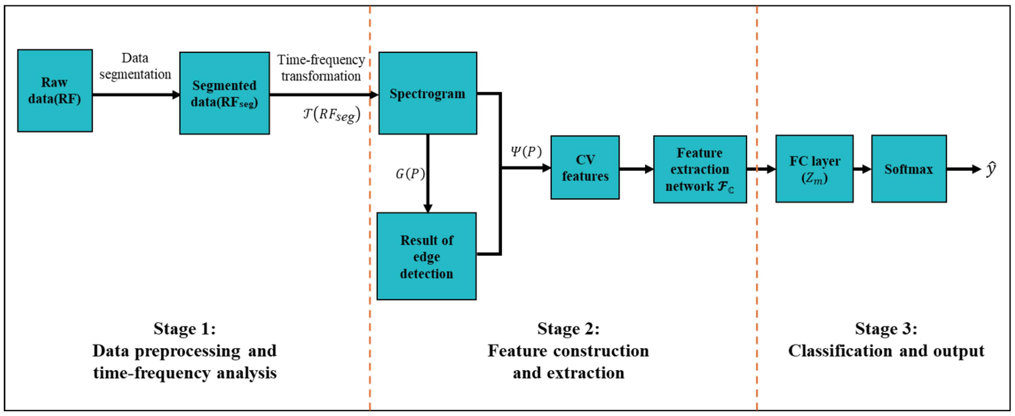
Figure 2.
Architecture of the proposed CV-CNN.
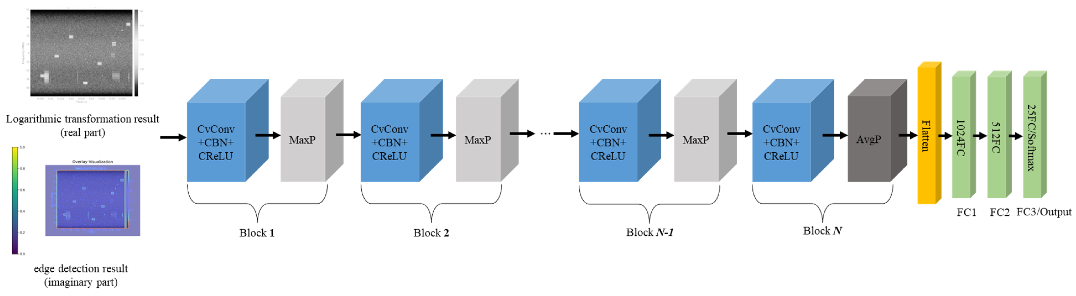
Figure 3.
Ablation experiment flowchart.

Figure 4.
Impact of network depth on accuracy.
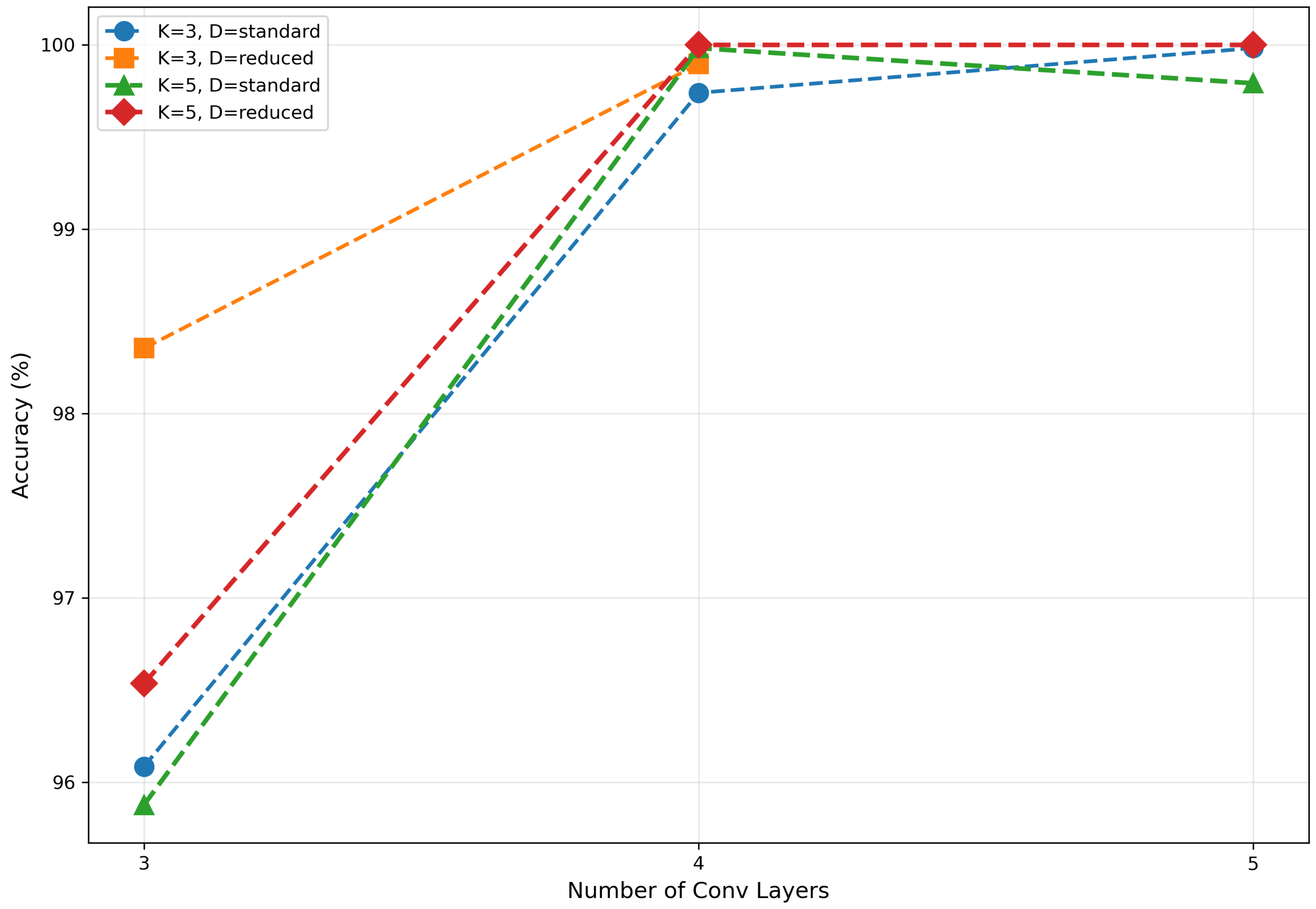
Figure 5.
Impact of kernel size on accuracy.
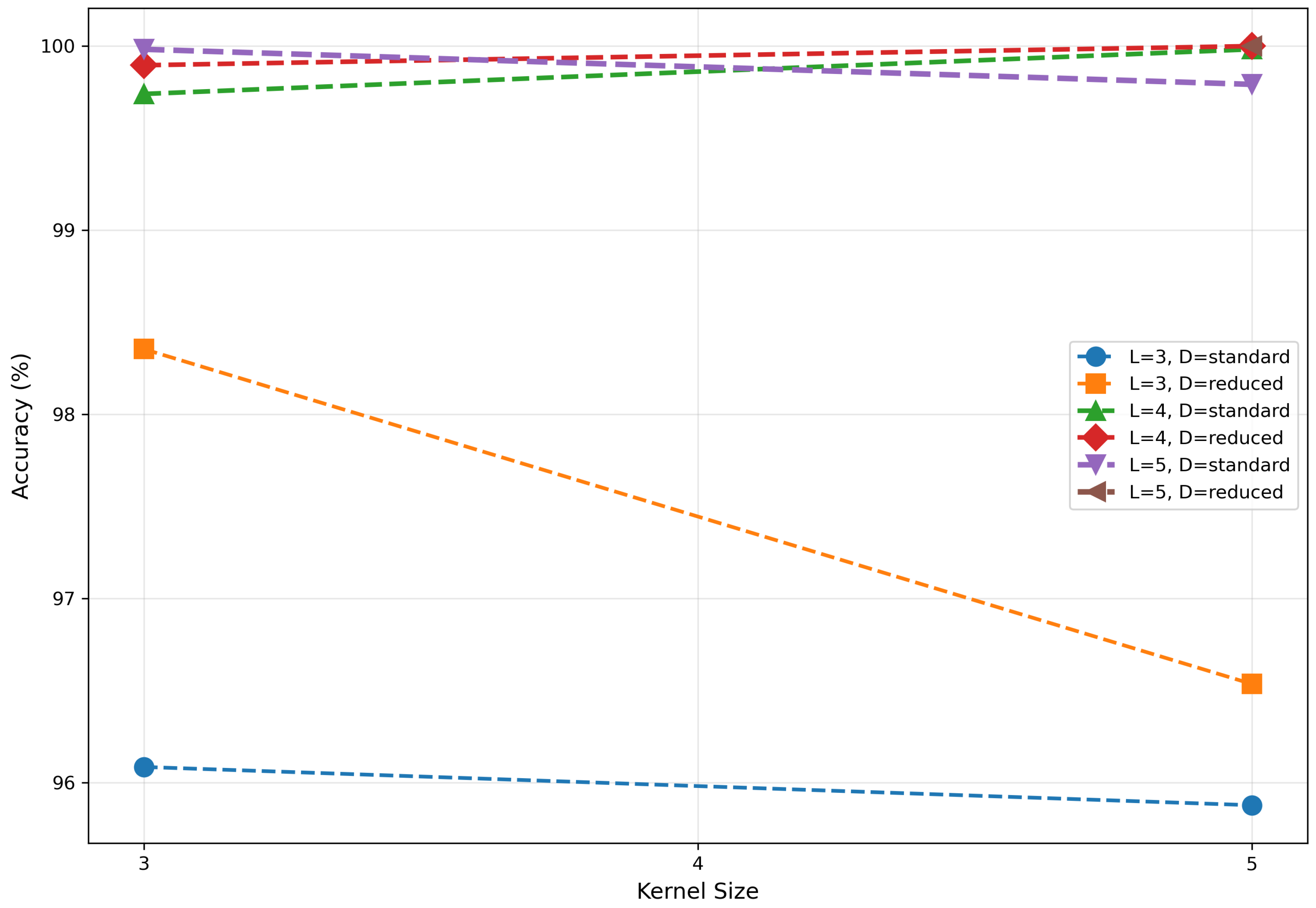
Figure 6.
Impact of dropout mode on accuracy.
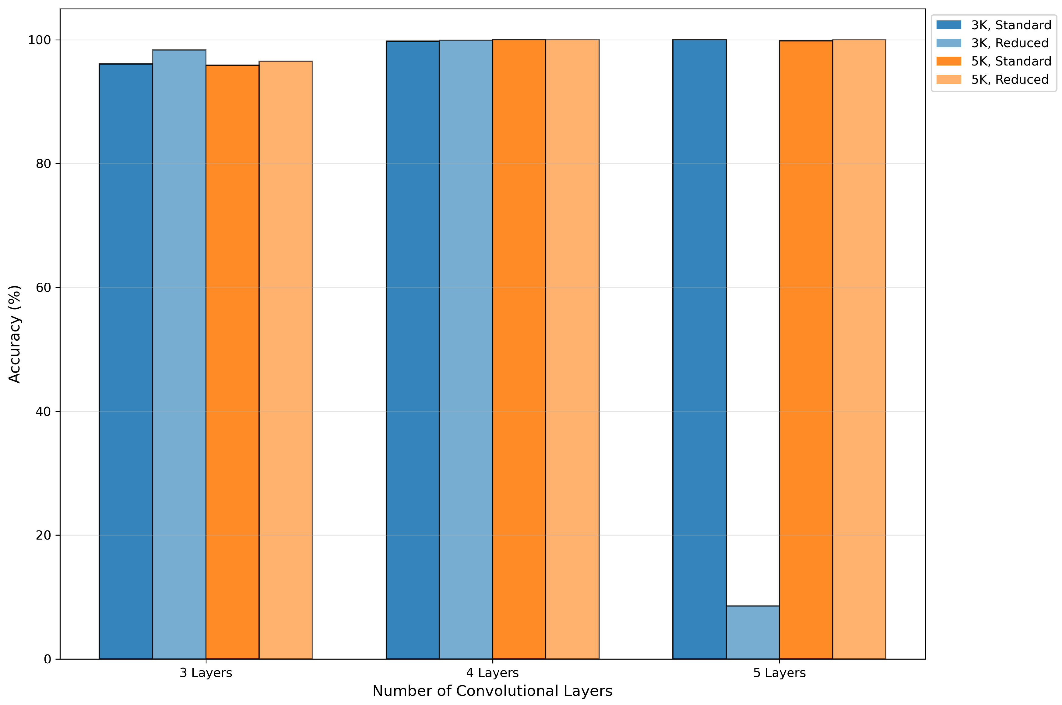
Figure 7.
Performance comparison of (a) CV-CNN and (b) RV-CNN at different network depth.
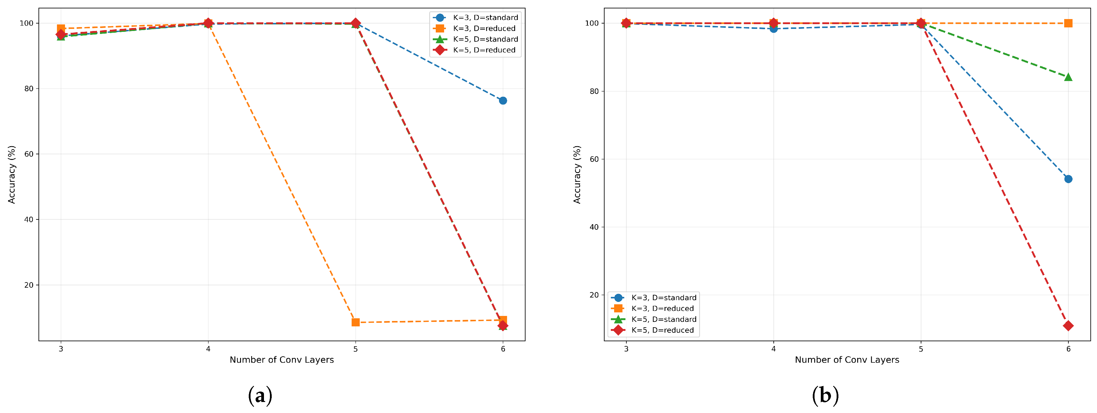
Figure 8.
Accuracy comparison of (a) CV-CNN and (b) RV-CNN at different SNRs.
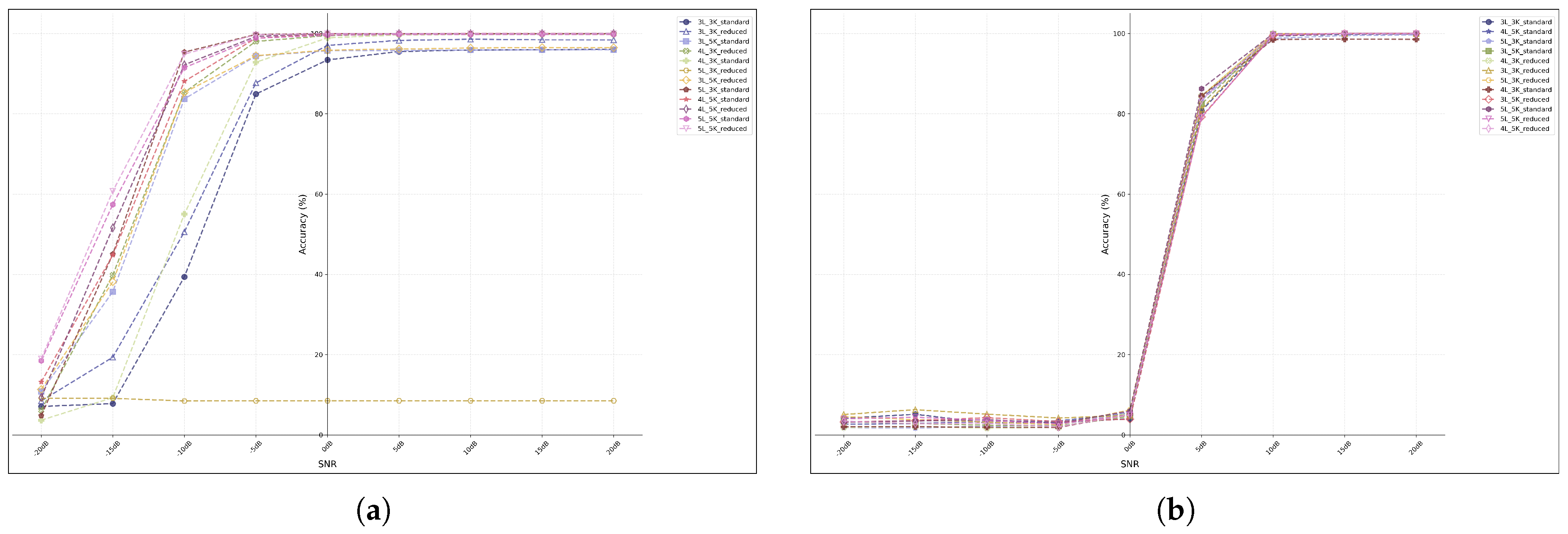

Table 1.
Architecture configuration of the (4L, 3K, Reduced) CV-CNN model.
| Layer type | Layer parameter | Activation |
| Input | 1x2x384x288 | – |
| CvConv1+CBN | k=3x3, s=1, p=1 → 1x64x384x288 | CReLU |
| MaxP | MaxPool 2x2 → 1x64x192x144 | – |
| Dropout1 | p=0.3 | – |
| CvConv2+CBN | k=3x3, s=1, p=1 → 1x128x192x144 | CReLU |
| MaxP | MaxPool 2x2 → 1x128x96x72 | – |
| Dropout2 | p=0.4 | – |
| CvConv3+CBN | k=3x3, s=1, p=1 → 1x256x96x72 | CReLU |
| MaxP | MaxPool 2x2 → 1x256x48x36 | – |
| Dropout3 | p=0.5 | – |
| CvConv4+CBN | k=3x3, s=1, p=1 → 1x256x48x36 | CReLU |
| AvgP | AdaptiveAvgPool 6x6 → 1x256x6x6 | – |
| Flatten | 1x9216 | – |
| FC1 | 9216 → 1024 | ReLU |
| DropoutFC | p=0.5 | – |
| FC2 | 1024 → 512 | ReLU |
| DropoutFC | p=0.5 | – |
| FC3/Output | 512 → 25 | Softmax |
Table 2.
Distinction between complex-valued and real-valued convolution.
| Aspect | Complex-valued | Real-valued |
|---|---|---|
| convolution | convolution | |
| Input/Output | Complex number | Real number |
| Number of parameters | 4 times real-valued | Relatively few |
| Phase processing | Preserving phase | Phase loss |
| Frequency domain | Correlation modeling | Magnitude-only |
| Computational complexity | Higher | Lower |
Table 3.
Accuracy of CV-CNN model under different parameter configurations.
| Network depth | Kernel size | Dropout mode | Accuracy (%) |
|---|---|---|---|
| 3 | 3 | Standard | 96.08 |
| 3 | 3 | Reduced | 98.35 |
| 3 | 5 | Standard | 95.88 |
| 3 | 5 | Reduced | 96.53 |
| 4 | 3 | Standard | 99.74 |
| 4 | 3 | Reduced | 99.90 |
| 4 | 5 | Standard | 99.98 |
| 4 | 5 | Reduced | 100.00 |
| 5 | 3 | Standard | 99.98 |
| 5 | 3 | Reduced | 8.52 |
| 5 | 5 | Standard | 99.79 |
| 5 | 5 | Reduced | 100.00 |
| 6 | 3 | Standard | 76.33 |
| 6 | 3 | Reduced | 9.23 |
| 6 | 5 | Standard | 7.52 |
| 6 | 5 | Reduced | 7.52 |
Table 4.
Comparison of accuracy between CV-CNN and RV-CNN models.
| Network Depth |
Kernel Size |
Dropout Mode |
CV-CNN Accuracy(%) |
RV-CNN Accuracy(%) |
| 3 | 3 | Standard | 96.08 | 99.88 |
| 3 | 3 | Reduced | 98.35 | 99.98 |
| 3 | 5 | Standard | 95.88 | 99.97 |
| 3 | 5 | Reduced | 96.53 | 100 |
| 4 | 3 | Standard | 99.74 | 98.35 |
| 4 | 3 | Reduced | 99.9 | 100 |
| 4 | 5 | Standard | 99.98 | 100 |
| 4 | 5 | Reduced | 100 | 100 |
| 5 | 3 | Standard | 99.98 | 99.62 |
| 5 | 3 | Reduced | 8.52 | 100 |
| 5 | 5 | Standard | 99.79 | 100 |
| 5 | 5 | Reduced | 100 | 100 |
| 6 | 3 | Standard | 76.33 | 99.98 |
| 6 | 3 | Reduced | 9.23 | 54.12 |
| 6 | 5 | Standard | 7.52 | 84.13 |
| 6 | 5 | Reduced | 7.52 | 10.93 |
Disclaimer/Publisher’s Note: The statements, opinions and data contained in all publications are solely those of the individual author(s) and contributor(s) and not of MDPI and/or the editor(s). MDPI and/or the editor(s) disclaim responsibility for any injury to people or property resulting from any ideas, methods, instructions or products referred to in the content. |
© 2025 by the authors. Licensee MDPI, Basel, Switzerland. This article is an open access article distributed under the terms and conditions of the Creative Commons Attribution (CC BY) license (http://creativecommons.org/licenses/by/4.0/).
Copyright: This open access article is published under a Creative Commons CC BY 4.0 license, which permit the free download, distribution, and reuse, provided that the author and preprint are cited in any reuse.


