Submitted:
16 December 2025
Posted:
17 December 2025
You are already at the latest version
Abstract
Delay Sobolev equations (DSEs), a kind of pseudo-parabolic equation with delay, are widely used in diffusion or transport with memory, flow in the fluid and other related fields. In this paper, two high-order compact difference methods (HOCD-I and HOCD-II) are introduced to solve the semi-linear DSEs. Moreover, the convergence of the methods are proved. Finally, in order to testify the accuracy and the convergence rate of the methods, two concrete numerical experiments are presented.
Keywords:
semi-linear delay Sobolev equations
; convergence
; high-order compact difference methods
; numerical experiments
1. Introduction
Consider the following initial-boundary value problems(IBVPs) of semi-linear delay Sobolev equation with
where are the coefficients, are some given real constants with , functions f, , and are given and smooth enough on their respective domains. The function f satisfies Lipschitz condition, i.e.
DSEs, a subclass of pseudo-parabolic equations incorporating time-delay effects, play a pivotal role in modeling a wide array of physical and engineering phenomena. They are particularly indispensable in describing diffusion or transport processes with memory effects, unsteady seepage in fissured rocks [1], and heat transfer mechanisms [2]. However, the intricate nature of the delay term and nonlinearity in these equations often renders analytical solutions unattainable in practical scenarios. As a result, numerical methods have become the primary avenue for obtaining approximate solutions and conducting quantitative analysis of such problems.
Up to now, substantial research efforts have been devoted to the numerical solution of Sobolev equations without delay, yielding a rich repertoire of effective methods. For instance, Mishra, Khebchareon and Pany [3] used a second-order backward difference scheme incorporated with a finite element method of conforming type to solve Sobolev equations. Yu and Wang [4] gave a efficient space-time spectral method. Ngondiep [5] proposed a high-order weak Galerkin finite element method. Alikhanov el al. [6] considered two high order compact difference schemes for Sobolev-type convection-diffusion equation with multi term and time fraction. Niu et al. [7] develop a fast high order compact difference scheme for solving the nonlinear distributed-order fractional Sobolev model appearing in porous media.
In contrast, the numerical study of DSEs remains relatively under explored, despite their critical relevance to real-world systems with memory and time-lag effects. Existing works in this area are limited and primarily focus on specific subclasses of DSEs or linearized models. Huseynov et al. [8] discovered the existence of mild solution for fractional-order DSEs. Johnson [9] focused on approximate controllability results for Sobolev-Type Hilfer Fractional Delay Differential Equations. Tan and Ran [10] presented linearized compact difference methods for solving distributed delay Sobolev equations. Chiyaneh and Duru[11] and Günes and Duru[12] offered a numerical method for pseudo-parabolic equations with singularly perturbance. Zhang et al.[13] analyzed the error of two linearized compact difference schemes for Sobolev equations. Amirali and Amiraliyev[14] constructed a high-order difference method to solve linear pseudo-parabolic equation with time delay. Ilati [15] introduced a local radial basis function-compact finite difference method. Yilmaz and Piskin [16] found the global existence and decay of solutions for a delayed generalized Sobolev equation involving Laplacian operator and logarithmic nonlinearity, within the framework of variable-exponent Sobolev spaces. Zhang and Hou [17] gave a three-level high-order compact difference method to simplify the process of method computation. Alikhanov et al. [18] analyzed a linearized high-order -compact difference scheme to solve multi-term time-fractional nonlinear Sobolev-type convection-diffusion equations.
Given the prevalence of time-delay effects in practical engineering and physical systems, the development of high-precision numerical methods for DSEs is of paramount importance. Motivated by the aforementioned research gaps and the advantages of HOCD methods in achieving high accuracy with compact stencils, this paper introduces two high-order compact difference methods (HOCD-I and HOCD-II) for solving semi-linear delay Sobolev equations. We rigorously prove the convergence of both methods through error estimation: HOCD-I attains second-order accuracy in the temporal direction and fourth-order accuracy in the spatial direction, while HOCD-II achieves fourth-order accuracy in both time and space. Finally, two concrete numerical experiments are carried out to validate the accuracy and convergence rates of the proposed methods, demonstrating their effectiveness and feasibility in practical applications.
2. I-Type High-Order Compact Difference Method
2.1. The Derivation of I-Type High-Order Compact Difference Method
Let and be the step sizes in time and space, respectively. Denote and . Let be the grid function space defined on . For any , we define
The following lemma will be used in derivation of the difference methods.
Lemma 1.
[19]. Suppose , then there exists a constant such that
Considering the case of (1.1) at point yields that
Let , and , we have
By the Taylor expansion at the point , we obtain that
Taking the difference and sum between (4) and (5) gives that
The equation (6) and (7) can be rearranged into
Similarly, we have
Substituting (8) , (10) and (11) into (3), we obtain that
where . Acting operator on the both sides of (12) infers that
From Lemma 1, we have
Substituting (14) into (13) gives that
where .
Suppose that where , then there exists a constant such that
By omitting the remainder term in (15) and replacing with its approximation , we get the I-type high order compact difference scheme as
We denote the first equation in (17) as (17a). The estimate (16) indicates that the method (17) has the local accuracy .
Theorem 1.
High order compact difference method (17) for problem (1) is uniquely solvable.
Proof.
Since and are positive definite operators, the coefficient matrix of method (17) is positive definite. Thus, the method (17) is uniquely solvable. □
2.2. Error Analysis for the I-Type High-Order Compact Difference Method
Introduce a grid function space on and we denote
Lemma 2.
([20]). Suppose , then
.
Lemma 3.
([19]). Suppose , then
Lemma 4.
([19]). (Gronwall inequality) Suppose that there exist such that nonnegative sequence satisfies
then we have
Define . Subtracting (2.15a) from (15) leads to
where the first equation is denoted as (19a). With the above argument, an error analysis result of method (17) can be stated as follow.
Theorem 2.
Assume that and the condition (2) holds. Then method (17) satisfies the following error estimation:
where .
Proof.
Multiplying on the both sides of (19a) and summing up for i from 1 to yields that
Considering (21), the two terms in the left hand side and the first term in the right hand side of respectively, it deduced from Lemma 3 and Abel’s partial summation formula()(see [21]) that
The second term in the right hand side of (21) follows by Lipschitz condition (2), Young’s inequality() with and Lemma(3) that
Applying Young’s inequality with , inequality and (16) infers that
Substituting (22)-(26) into (21) yields that
Multiplying on the both sides of (27) and summing up for 0 from 1 to k, we have
Since Lemma(4) and (Lemma(2)), (28) can be followed by
By means of Lemma(4), (29) can be written as
namely,
where .
From Lemma(4), we get
where . Hence, method (17) is convergent. □
3. II-Type High-Order Compact Difference Method
3.1. The Derivation of II-Type High-Order Compact Difference Method
In this section, we will give another numerical scheme to solve the problem (1). Firstly, we consider problem (1) at the mesh point yields that
Lemma 5.
[19]. Suppose , then there exists a constant such that
By Lemma (5), we have that
Acting on both side of (33) gives that
Substituting (34) into (35) leads to
where .
Acting on both side of (36) and substituting (14) into it infers
where .
Suppose that where , then there exists a constant such that
By omitting the remainder term in (37) and replacing with its approximation , we get the II-type compact difference scheme as
where the initial-boundary conditions are
3.2. Error Analysis for the II-Type High-Order Compact Difference Method
Define . Subtracting (39) from (37) leads to
With the above argument, an error analysis result of method (39) can be stated as follow.
Theorem 3.
Assume that the Lipschitz condition holds and , then method (39) satisfies the following error estimation:
where .
Proof.
Multiplying on the both sides of the first equation in (41) and summing up for i from 1 to yields that
Considering the first term in the left hand side(LHS) of (43) and by the second inequality in Lemma 3, we have
In regard to the second term in the LHS of (43), we have
It follows from Cauchy-Schwarz inequality that the first term in the right hand side of (43) that
Also, it deduced from the Lipschitz condition (2), Lemma 3, we have
For the above inequality (47) By Young’s inequality () with Cauchy-Schwarz inequality() and the second inequality in Lemma 2 that
Considering the third term in the right hand side of (43), by using the Young’s inequality with , it holds that
Substituting (44)-(49) into (43) gives
Summing both sides of (50) from to infers that
which can be rearranged into
Multiplying both sides of (52) by yields
Suppose that there exists a constant and satisfying
Then there’s an estimation
where
By using Grownwall inequality to (54), we can deduce
From Lemma(4), we get
where . Hence (42) holds for . □
4. Numerical Experiments
To empirically validate the accuracy, convergence, and practical feasibility of the two high-order compact difference methods (HOCD-I and HOCD-II) proposed in this study, we conducted numerical simulations on two initial-boundary value problems (IBVPs) of semi-linear delay Sobolev equations. All experiments were implemented in MATLAB R2020a, with the numerical schemes corresponding to the difference formulas derived in Section 2 and 3 (denoted as HOCD-I and HOCD-II, respectively).
To show the actual calculation accuracy and convergence rates of HOCD-I and HOCD-II methods, we introduce the following formulas to compute the global errors, and convergence orders of the two methods, respectively:
where , , and .
Example 1.
Consider the following IBVPs of semi-linear delay Sobolev equations:
where , and the example 1 has exact solution .
We applied HOCD-I and HOCD-II to solve this example 1 with spatial step sizes , corresponding to ). The global maximum errors () and convergence orders (p) of the two methods are summarized in Table 1. As shown in Table 1, both methods yield extremely small global errors (on the order of to ), confirming their high precision. For HOCD-I, the convergence order in space is consistently close to 4 (ranging from 3.99 to 4.01), which matches its theoretical spatial accuracy of fourth order; combined with , this further verifies its second-order temporal accuracy. For HOCD-II, the convergence order remains approximately 4 (ranging from 4.07 to 4.24), validating its theoretical fourth-order accuracy in both time and space.
To visually demonstrate the performance of the methods, we plotted the exact solution, numerical solutions of HOCD-I and HOCD-II, and their corresponding error surfaces under the parameter setting (see Figure 1). As illustrated in Figure 1(a)-1(c), the numerical solutions of both methods are visually indistinguishable from the exact solution, indicating excellent agreement. The error surfaces in Figure 1(d) and 1(e) further confirm that the maximum errors of HOCD-I and HOCD-II are on the orders of and , respectively—values sufficiently small for practical engineering and scientific computing applications.
Example 2.
Consider the following IBVPs of delay semi-linear Sobolev equations:
where , and the example 2 has exact solution .
We solved this example 2 using the same parameter configuration as example (57): spatial step sizes , with for HOCD-I and for HOCD-II. The numerical results—including global maximum errors and convergence orders—are presented in Table 2.
Table 2 confirms the consistent performance of the two methods across different nonlinearities. For HOCD-I, the global error remains on the order of to , with a spatial convergence order close to 4 (minimum 3.80, maximum 4.01), verifying its stability even for complex exponential-logarithmic nonlinearity. For HOCD-II, the global error is further reduced to to , and the convergence order is strictly maintained at 4.01, highlighting its superior accuracy and robustness. We also visualized the results under (see Figure 2). Figure 2(a)-2(c) show that the numerical solutions of HOCD-I and HOCD-II are visually identical to the exact solution, while Figure 2(d) and 2(e) demonstrate that the errors of the two methods are on the orders of and , respectively. These visual results further corroborate the quantitative findings in Table 2, confirming that both methods can reliably solve semi-linear delay Sobolev equations with diverse nonlinear terms.
5. Conclusion
In this paper, we proposed two high-order compact difference schemes to solve the semi-linear delay Sobolev equations. Moreover, the convergence of the two methods are proved. Finally, the numerical experiments illustrate that the HOCD-I methods has the computational accuracy and the HOCD-II methods has the computational accuracy , which indicates they are viable and effective in practical applications.
Author Contributions
Xiaoyu Zhang defined the research theme, designed numerical method, conducted the theory analysis, numerical experiments and wrote the paper.
Funding
This research received no external funding.
Acknowledgments
The authors gratefully acknowledge the anonymous reviewers for their insightful comments and valuable suggestions, which have significantly improved the quality of this manuscript.
Conflicts of Interest
The authors declare no confficts of interest.
References
- Barenblatt, G.; Zheltov, I.; Kochina, I. Basic concepts in the theory of seepage of homogeneous liquids in fissured rocks. J. Appl. Math. Mech. 1960, 24, 1286–1303. [Google Scholar] [CrossRef]
- Ting, T. W. A cooling process according to two-temperature theory of heat conduction. J. Math. Anal. Appl. 1974, 45, 23–31. [Google Scholar] [CrossRef]
- Mishra, S.; Khebchareon, M.; Pany, A.K. Second order backward difference scheme combined with finite element method for a 2D Sobolev equation with Burgers’ type non-linearity. Comput. Math. Appl. 2023, 141, 170–190. [Google Scholar] [CrossRef]
- Yu, X.; Wang, M. Efficient spectral and spectral element methods for Sobolev equation with diagonalization technique. Appl. Numer. Math. 2024, 201, 265–281. [Google Scholar] [CrossRef]
- Ngondiep, E. An efficient high-order weak Galerkin finite element approach for Sobolev equation with variable matrix coefficients. Comput. Math. Appl. 2025, 180, 279–298. [Google Scholar] [CrossRef]
- Alikhanov, A. A.; Yadav, P.; Singh, V. K. A high-order compact difference scheme for the multi-term time-fractional Sobolev-type convection-diffusion equation. Comput. Math. Appl. 2025, 44, 115. [Google Scholar] [CrossRef]
- Niu, Y.; Liu, Y.; Li, H.; Liu, F. st high-order compact difference scheme for the nonlinear distributed-order fractional Sobolev model appearing in porous media. Math.Comput. Simul. 2023, 203, 378–407. [Google Scholar] [CrossRef]
- Huseynov, I. T.; Ahmadova, A.; Mahmudov, N. I. On a study of Sobolev-type fractional functional evolution equations. Math. Meth. Appl. Sci. 2022, 45, 5002–5042. [Google Scholar] [CrossRef]
- Johnson, M.; Kavitha, K.; Chalishajar, D.; Malik, M.; Vijayakumar, V.; Shukla, A. An analysis of approximate controllability for Hilfer fractional delay differential equations of Sobolev type without uniqueness. Nonlinear Anal.-Model Control. 2023, 28, 632–654. [Google Scholar] [CrossRef]
- Tan, Z.; Ran, M. Linearized compact difference methods for solving nonlinear Sobolev equations with distributed delay. Numer. Methods Partial Differ. Eq. 2023, 39, 2141–2162. [Google Scholar] [CrossRef]
- Chiyaneh, A. B.; Duru, H. A numerical scheme on s-mesh for the singularly perturbed initial boundary value Sobolev problems with large time delay: Solving singularly perturbed IBV Sobolev problems with lagre time delay using S-mesh method. J. Math. Mech. Comput. Sci. 2023, 117, 93–111. [Google Scholar] [CrossRef]
- Günes, B.; Duru, H. A second-order numerical method for pseudo-parabolic equations having both layer behavior and delay parameter. J. Commun. Fac. Sci. Univ. Ank.-Ser, A1 Math. Stat. 2024, 73, 569–587. [Google Scholar] [CrossRef]
- Zhang, J.J.; Qin, Y.; Zhang, Q. Maximum error estimates of two linearized compact difference schemes for two-dimensional nonlinear Sobolev equations. Appl. Numer. Math. 2023, 184, 253–272. [Google Scholar] [CrossRef]
- Amirali, I.; Amiraliyev, G.M. Numerical solution of linear pseudo-parabolic equation with time delay using three layer difference method. J. Comput. Appl. Math. 2024, 436, 115417. [Google Scholar] [CrossRef]
- Ilati, M. A local radial basis function-compact finite difference method for Sobolev equation arising from fluid dynamics. Eng. Anal. Bound. Elem. 2024, 169, 106020. [Google Scholar] [CrossRef]
- Yilmaz, N.; Piskin, E. Global existence and decay of solutions for a delayed m-Laplacian equation with logarithmic term in variable-exponent Sobolev spaces. Filomat. 2024, 38, 8157–8168. [Google Scholar] [CrossRef]
- Zhang, C.; Hou, B. High-order compact difference methods for 2D Sobolev equations with piecewise continuous argument. Acta. Math. Sci. 2025, 45, 1855–1878. [Google Scholar] [CrossRef]
- Alikhanov, A. A.; Asl, M. S.; Huang, C.; Alikhanov, A. A. A discrete Grönwall inequality for L2-type difference schemes with application to multi-term time-fractional nonlinear Sobolev-type convection-diffusion equations with delay. Commun. Nonlinear Sci. Numer. Simul. 2025, 41, 109231. [Google Scholar] [CrossRef]
- Sun, Z.; Zhang, Z. A linearized compact difference scheme for a class of nonlinear delay partial differential equations. Appl. Math. Model. 2013, 37, 742–752. [Google Scholar] [CrossRef]
- Sun, Z. The numerical methods for partial differential equations; Science Press: Beijing, 2012. [Google Scholar]
- Niculescu, C. P.; Stanescu, M. M. A note on Abel’s partial summation formula. Aequ. Math. 2017, 91, 1009–1024. [Google Scholar] [CrossRef]
- Dai, L.; Fan, L. Analytical and numerical approaches to characteristics of linear and nonlinear vibratory systems under piecewise discontinuous disturbances. Commun. Nonlinear Sci. Numer. Simul. 2004, 9, 417–429. [Google Scholar] [CrossRef]
Figure 1.
Applying the HOCD-I and HOCD-II methods to solve example 1 with , the exact solutions (a), the numerical solutions of HOCD-I method(b), the numerical solutions of HOCD-II method(c),the error surface of HOCD-I method(d),the error surface of HOCD-II method(e).
Figure 1.
Applying the HOCD-I and HOCD-II methods to solve example 1 with , the exact solutions (a), the numerical solutions of HOCD-I method(b), the numerical solutions of HOCD-II method(c),the error surface of HOCD-I method(d),the error surface of HOCD-II method(e).
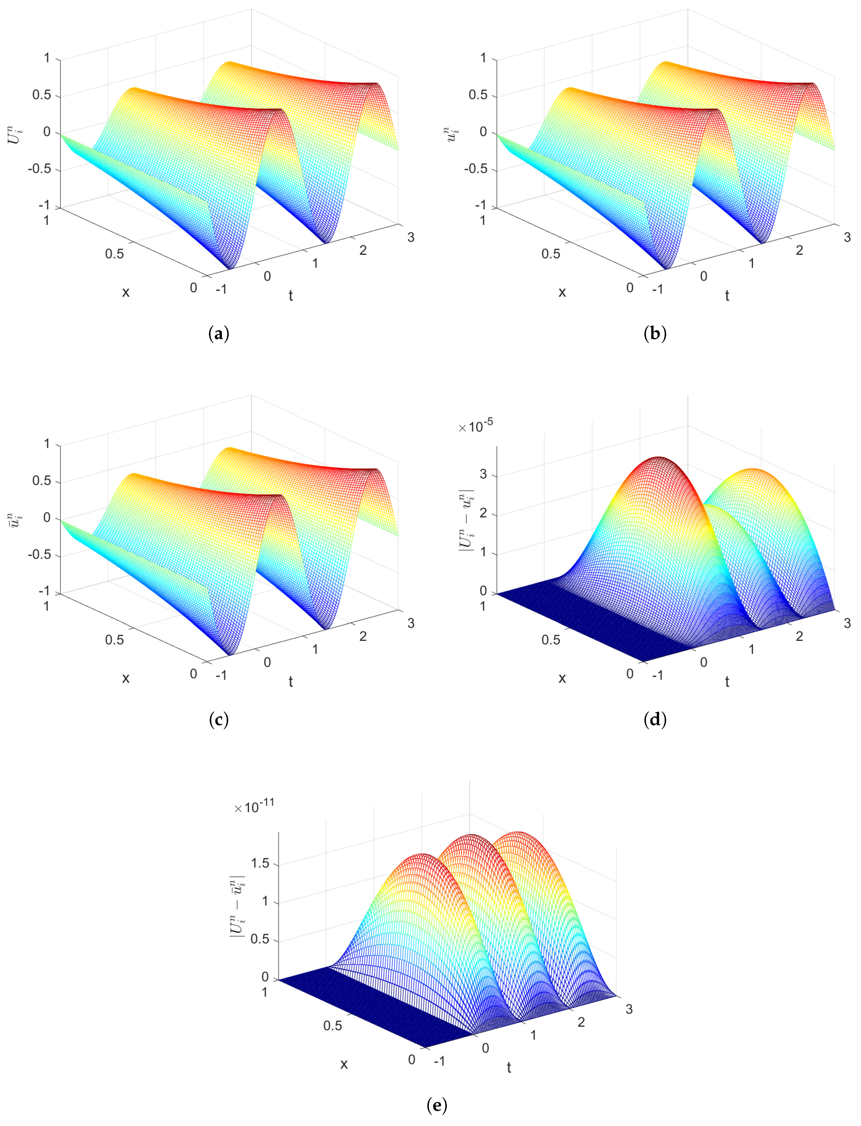
Figure 2.
Applying the HOCD-I and HOCD-II methods to solve example 2 with , the exact solutions (a), the numerical solutions of HOCD-I method(b), the numerical solutions of HOCD-II method(c), the error surface of HOCD-I method(d), the error surface of HOCD-II method(e).
Figure 2.
Applying the HOCD-I and HOCD-II methods to solve example 2 with , the exact solutions (a), the numerical solutions of HOCD-I method(b), the numerical solutions of HOCD-II method(c), the error surface of HOCD-I method(d), the error surface of HOCD-II method(e).
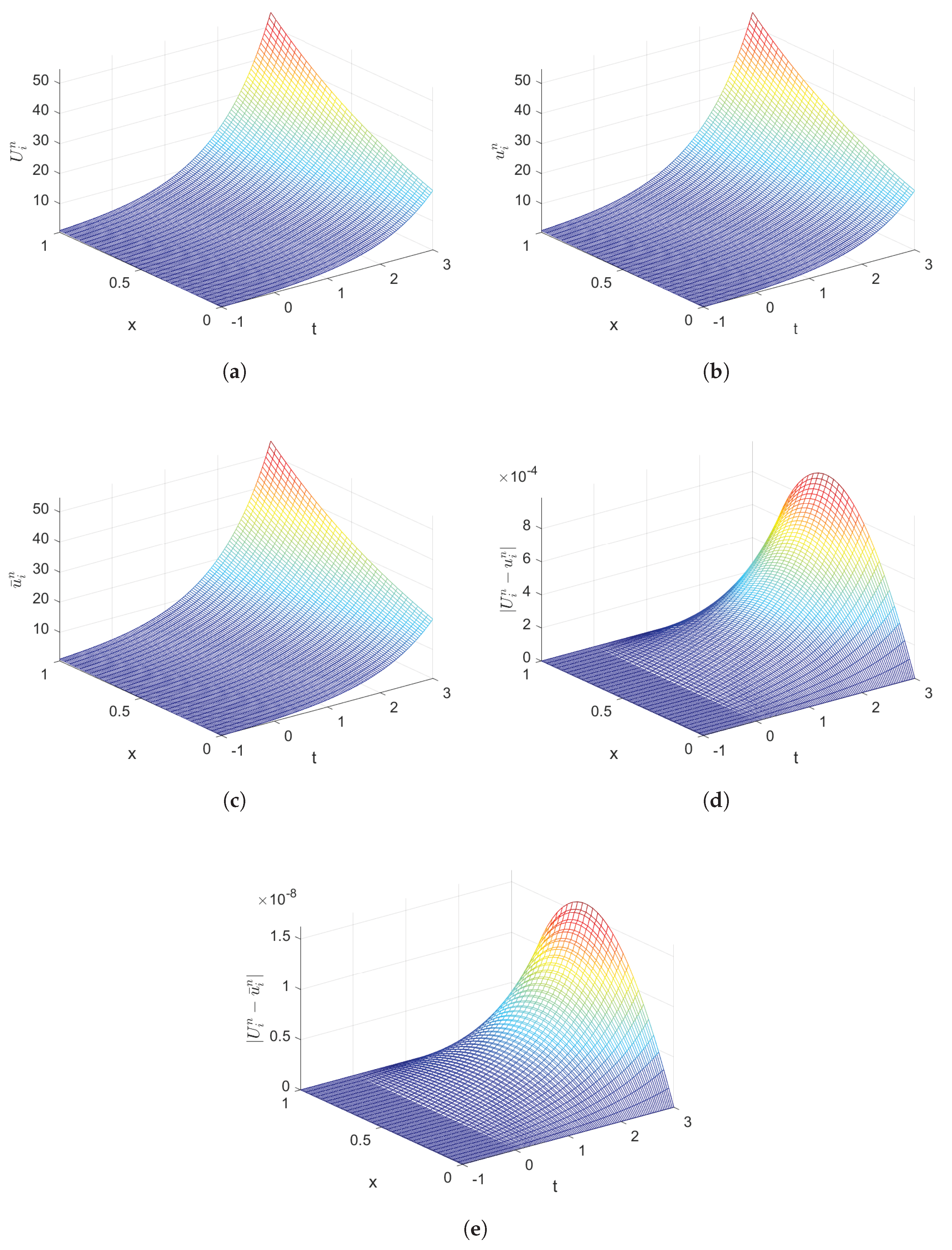

Table 1.
Global errors and convergence orders of example 1.
| h | HOCD-I method() | HOCD-II method() | ||
|---|---|---|---|---|
| p | ||||
| 4.2045e-06 | – | 1.0707e-07 | – | |
| 2.6424e-07 | 3.99 | 5.6532e-09 | 4.24 | |
| 5.2279e-08 | 4.00 | 1.0583e-09 | 4.13 | |
| 1.6533e-08 | 4.00 | 3.2483e-10 | 4.11 | |
| 6.7742e-09 | 4.00 | 1.3069e-10 | 4.08 | |
| 3.2595e-09 | 4.01 | 6.2227e-11 | 4.07 | |
Table 2.
Global errors and convergence orders of example 2.
| h | HOCD-I method() | HOCD-II method() | ||
|---|---|---|---|---|
| p | ||||
| 2.3095e-05 | – | 4.1861e-06 | – | |
| 1.4506e-06 | 3.99 | 2.6050e-07 | 4.01 | |
| 2.8699e-07 | 4.00 | 5.1321e-08 | 4.01 | |
| 9.0858e-08 | 4.00 | 1.6195e-18 | 4.01 | |
| 3.7166e-08 | 4.01 | 6.6321e-09 | 4.01 | |
| 1.8575e-08 | 3.80 | 3.1946e-09 | 4.01 | |
Disclaimer/Publisher’s Note: The statements, opinions and data contained in all publications are solely those of the individual author(s) and contributor(s) and not of MDPI and/or the editor(s). MDPI and/or the editor(s) disclaim responsibility for any injury to people or property resulting from any ideas, methods, instructions or products referred to in the content. |
© 2025 by the authors. Licensee MDPI, Basel, Switzerland. This article is an open access article distributed under the terms and conditions of the Creative Commons Attribution (CC BY) license (http://creativecommons.org/licenses/by/4.0/).
Copyright: This open access article is published under a Creative Commons CC BY 4.0 license, which permit the free download, distribution, and reuse, provided that the author and preprint are cited in any reuse.


