Submitted:
15 December 2025
Posted:
17 December 2025
You are already at the latest version
Abstract
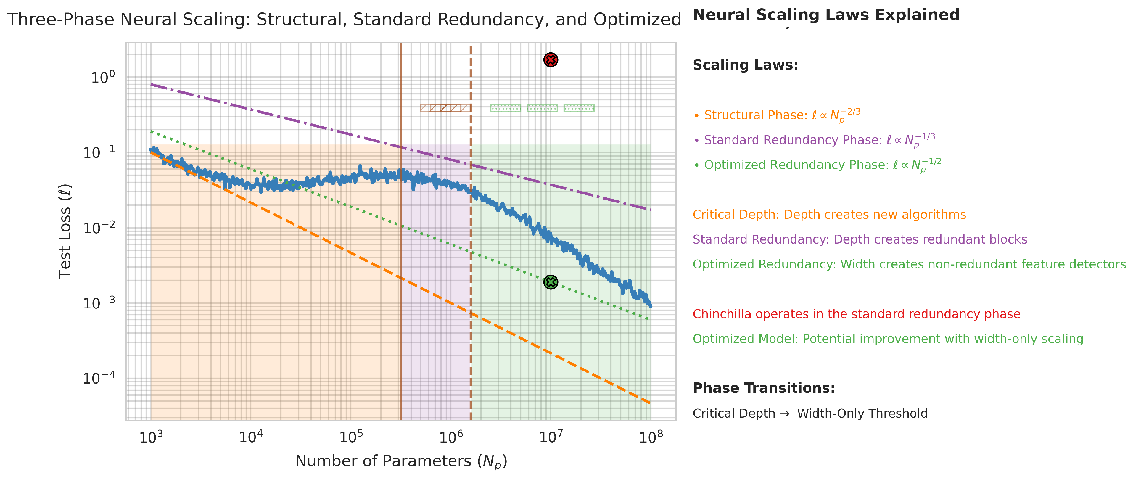
In this work, we present a refined interpretation of the Neural Scaling Laws that is inspired by phase transitions. Our starting point is from the paper: A Resource Based Model For Neural Scaling Laws. Indeed, there is both empirical and theoretical backing for the \( \ell \propto N_p^{-1/3} \) power law. Our formalization through the combined use of propositional logic and an SMT-solver allows us to draw new perspectives on the learning curve. As formulated and relied on for their internal consistency in the prior work, the critical depth conjecture is strengthened in our work. Rooted in a combination of: logic and empirical/theoretical insights, we draw a three regime profile of the Neural Scaling Laws. Ultimately, our physics-inspired proposal of Neural Scaling Laws profiles as follows: 1) structural phase, where we argue that, the loss scales following: \( \ell \propto N_p^{-2/3} \), 2) Above the \textit{critical depth}, a redundancy phase, with a loss following the classical: \( \ell \propto N_p^{-1/3} \) (where most of current LLMs operate). Finally, 3) an optimized trajectory where depth is fixed and a scaling is based on width following: \( \ell \propto N_p^{-1/2} \).
Keywords:
1. Introduction
1.1. Background
1.2. Motivation
1s mathematics {discovered or invented} ⟺ {revealed or engineered}?
- -
- The advent of the modern computing device or, commonly known as the computer,
- -
- The increasing size of our knowledge corpus – development of storage capabilities.
- -
- The digital -spectrum nature of our computing devices,
- -
- The accelerating pace at which our body of knowledge grows; it almost naturally arises that, we need to be building on solid/sound ground.
- -
- A form of “awareness” of the technological advancements and evolving environment i.e.: we move from, the local thinking/logic to innate network aware data types/structures.
- -
- On a syntactic level: we move away from manually allocating memory buffers to, powerful one-line design patterns of high-level programming languages – increased abstraction.
1.3. Recall and Preliminary Information
- -
- For the understanding of Deep Neural Networks – the articulation/interaction between data and model architecture,
- -
- From an efficiency perspective – considering both: fuel (data) and energy factors.
The landscape of Neural Scaling Laws (NSLs)
- -
- Learning Curve Theory [19]
- -
- A Resource Model For Neural Scaling Law [13]
- -
- A Neural Scaling Law from the Dimension of the Data Manifold [20]
- -
- Explaining neural scaling laws [21]
- -
- Scaling Laws for Deep Learning [22]
- -
- A Solvable Model of Neural Scaling Laws [23]
- -
- Information-Theoretic Foundations for Neural Scaling Laws [24]
1.4. NSLs – The Power Laws Recap
- -
- L: the test loss (e.g., cross-entropy or MSE),
- -
- N: the number of model parameters,
- -
- D: the number of training tokens (dataset size),
- -
- d: the intrinsic dimension of the data manifold Sharma and Kaplan [20].
- -
- L: the test loss (typically cross-entropy in nats),
- -
- N: the number of non-embedding model parameters,
- -
- D: the number of training tokens,
- -
- C: the training compute budget (FLOPs), with .
1.4.1. Summary of Key Scaling Exponents
- Data Manifold Dimension (d): Both Sharma and Kaplan [20] and Bahri et al. [21] link the scaling exponent to the intrinsic dimension d of the data. The difference in the predicted factor (4 vs. 1) arises from different assumptions about the nature of the approximation (e.g., piecewise constant vs. piecewise linear).
- Information-Theoretic View: Jeon and Roy [24] decomposes the loss into an estimation error () and a misspecification error (). This leads to a compute-optimal scaling where , implying equal scaling exponents of 1 for both N and D in the variance-limited regime.
- Random Feature Models: Maloney et al. [23] shows that the scaling exponent is directly inherited from the power-law decay of the data’s feature spectrum. This provides a direct, solvable link between data distribution statistics and model performance.
- Power Laws and Zipf’s Law: Hutter [19] demonstrates that if the underlying data features follow a Zipf distribution, the resulting learning curve will also be a power law, with the exponent being a function of the Zipf parameter.

| Paper | Scaling Law | Exponent |
|---|---|---|
| Sharma and Kaplan [20] | ||
| Bahri et al. [21] (2024) | , | |
| Jeon and Roy [24] | Optimal allocation: , | |
| Maloney et al. [23] | For a kernel spectrum | , |
| Hutter [19] | For Zipf-distributed features with exponent | , where |
| Song et al. [13] | (resource scaling), and | for |
| Paper | Scaling Law | Exponent | Optimal Scaling Policy |
|---|---|---|---|
| Kaplan et al. [16] | |||
| Hoffmann et al. [17] | |||
| (Chinchilla) | |||
| Besiroglu et al. [18] | |||
| (Replication attempt) |
- Kaplan et al. [16] established what’s most likely the foundational empirical scaling laws, finding that loss scales with a very shallow power law in N and D. Their analysis suggested a highly model-heavy optimal scaling policy ().
- Hoffmann et al. [17] revisited this with an extensive experimental sweep and found significantly steeper scaling exponents. Their key conclusion was that model and data should be scaled equally, leading to the “Chinchilla scaling” law where .
- Besiroglu et al. [18] attempted to replicate the parametric fit from Hoffmann et al. [17]. They found that the originally reported parameters were inaccurate due to an optimizer issue, and their corrected fit yields exponents that are consistent with the equal-scaling policy but with a slightly higher data exponent ().
1.5. Epicenter of Our Attention
Acknowledged Logical Inconsistency
2. Methods
2.1. Resource-Based Model – Specific Nomenclature
| Symbol / Term | Definition |
|---|---|
| ℓ, | Total test loss of the composite task. |
| N, | Total number of allocated neurons across all subtasks i.e. the “resource”. |
| Number of allocated neurons for a specific subtask. | |
| Number of neurons in a single layer (network width). | |
| Number of layers in the network (network depth). | |
| Total number of model parameters. | |
| Importance weight (penalty) assigned to a subtask during training. | |
| Module | A functional subnetwork responsible for a specific subtask. |
2.2. Resource-Based Model – Axioms & Conjectures
2.2.1. Hypotheses
- (Single task scaling),
- Homogeneous growth of resource allocation – the ratios of are constant as the network grows.
- Linear additivity of subtask losses – the total loss is the sum of subtask losses.
2.2.2. Axioms
- Assumption 1:
- Assumption 2:
- Assumption 3:
2.2.3. Conjecture – Critical Depth Conjecture
Critical Depth Conjecture
2.3. Resource-Based Model Logic Relies on “Critical Depth” Conjecture
2.4. Key Tricks for Formalizing Resource-Based Model in Z3
- -
- Through mechanized mathematics, we would like to confirm the Resource-based Model’s internal logic,
- -
- As a “byproduct”, working with machine-assistance, we could expect “angles” to be revealed that might not be readily visible.
- -
- In order to verify the properties we are interested in, it often necessary to reduce the the “space” search of the verifier/solver,
- -
-
Linked to the previous point, the problem so expressed lives in a pure “mathematical realm”. That is, the solver/prover has no awareness or intelligence about the nature of solution found.In other words, a solution can be perfectly fine from a mathematical point of view but might not describe a physical plausibility or sensical configuration of our problem.
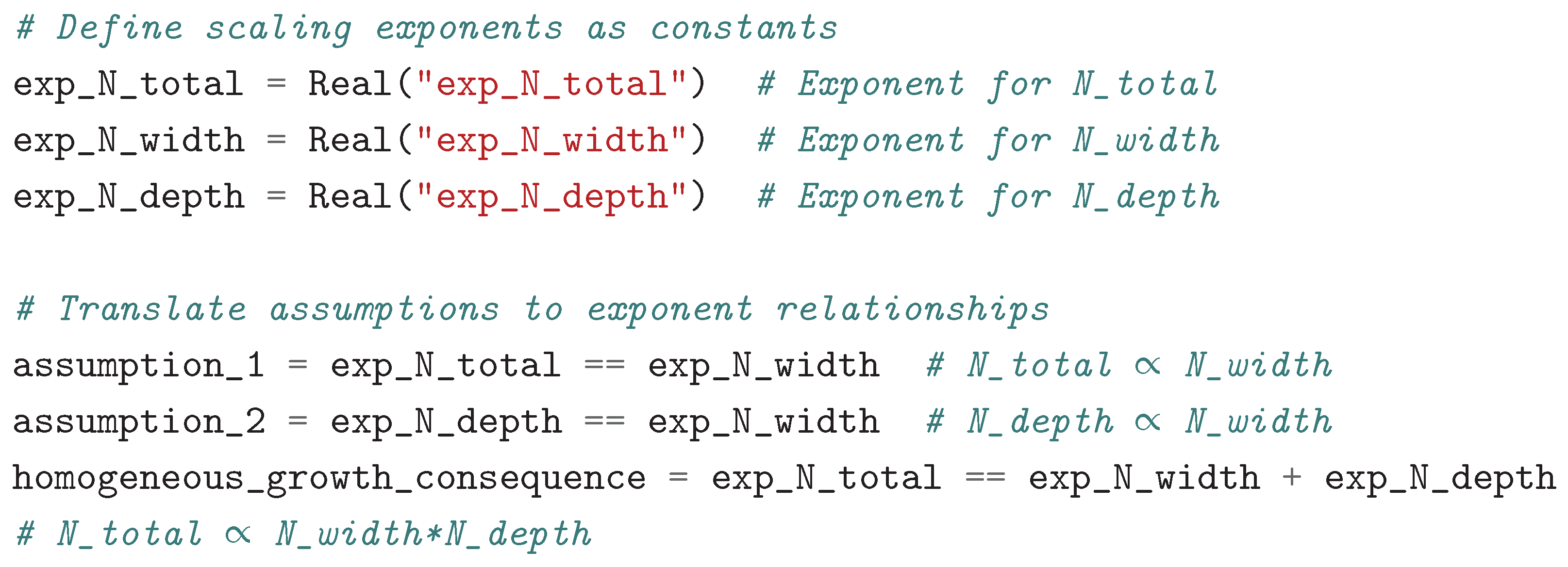
2.4.1. Modeling Scaling Exponents Instead of Absolute Values (The Core Trick)
 This is motivated because of:
- -
- Scaling laws are about how quantities change relative to each other as size increases,
- -
- By focusing on exponents (where ), we capture the essence of power-law relationships,
- -
- This eliminates trivial solutions such as: zero while preserving the scaling behavior.
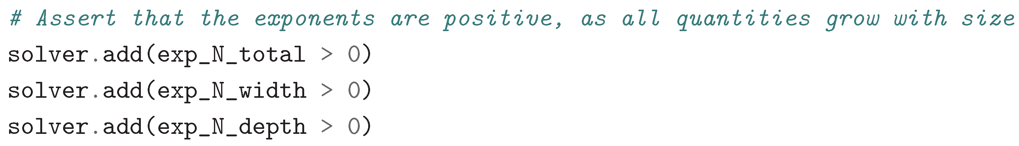
2.4.2. Enforcing Physical Plausibility with Positivity Constraints
 This is motivated because of:
- -
- In the context of neural network scaling, the width, depth, resources quantities should increase as model size increases,
- -
- Without this constraint, mathematically valid but physically meaningless solutions would satisfy the equations,
- -
- This is the key to discarding “trivial cases” that don’t embody a physical reality.
2.4.3. Correctly Translating Functional Relationships to Exponent Relationships
 This is motivated by the multiplicative law of exponents: i.e. to multiply exponents with the same basis is to addition their exponents.
2.4.4. Identifying the Precise Nature of the Contradiction
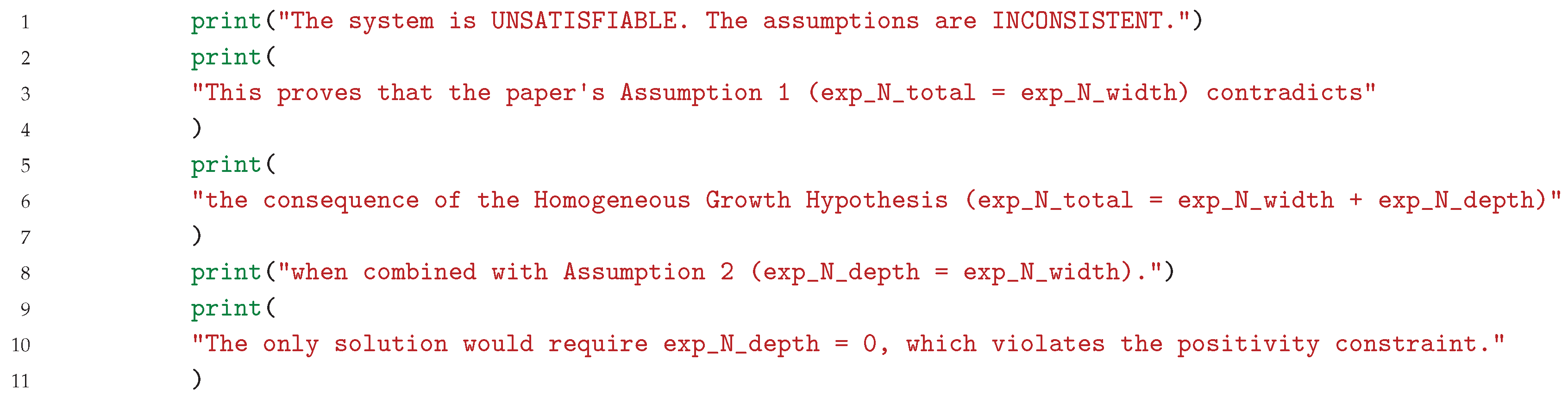
2.4.5. Separating Internal Consistency from Physical Plausibility
2.5. NSLs Derivation Based on Refactored Logic
- The Resource-based Model relying on the critical depth conjecture which predicts:
-
Our Refactored-resource Model uses the original paper assumptions without being indexed on the critical depth conjecture. Thus, we considers that the total number of allocated resources N should scale not only with the width but also with the depth of the network.It follows that, we derive a prediction relation loss of: .
- -
- The equation (A1) doesn’t hold when depth is scaled up, or,
- -
- The critical depth conjecture is topical and most of current Large Language Models (LLMs) are operating in a special regime – which we explore in the next sections to propose a proto-Unified Scaling Law (Section 3.3).
2.6. Pivoting Around the Critical Depth Conjecture
- -
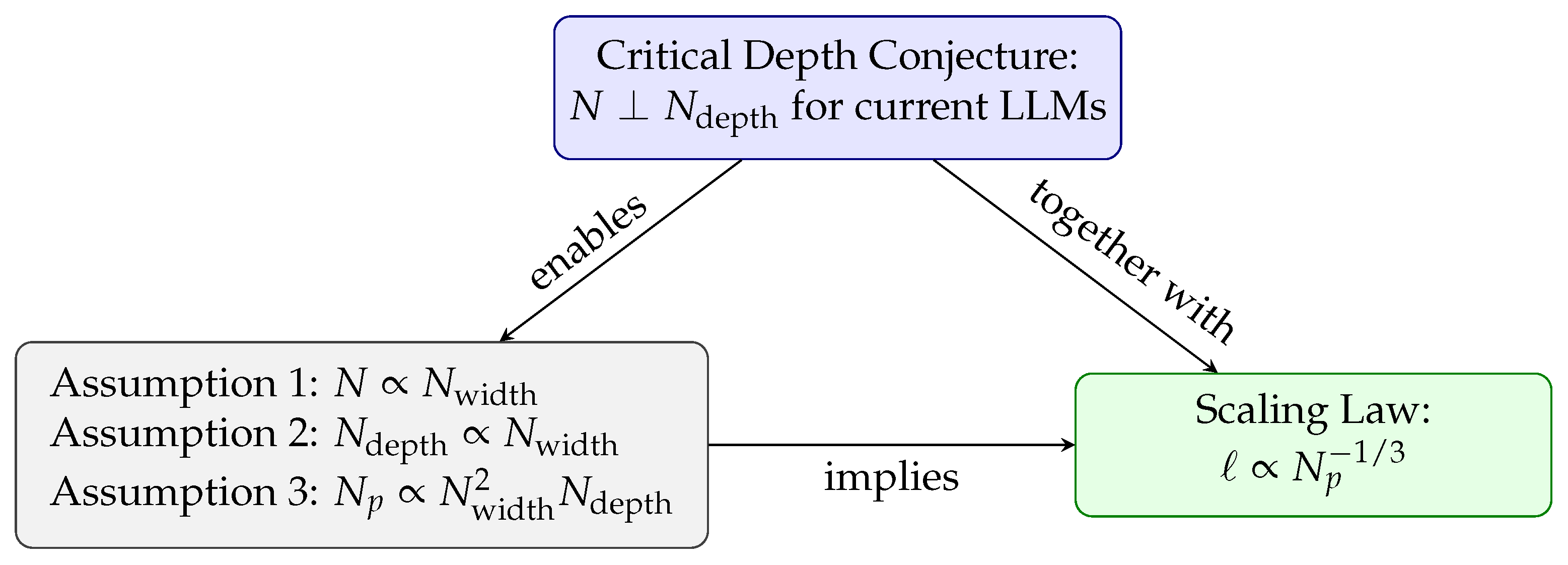
- Assumption 1: (resource scales only with width)
- -
- Assumption 2: (depth scales with width)
- -
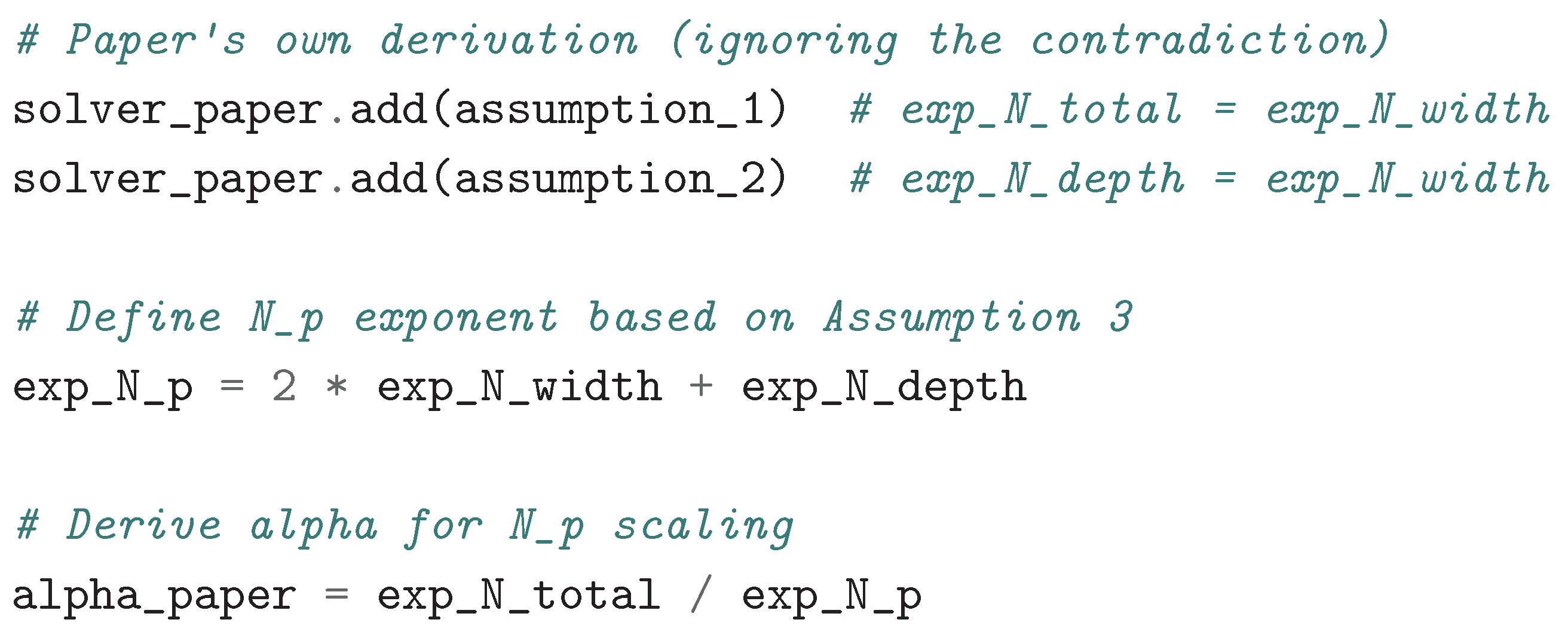
- Assumption 3:
- -
- The total effective resource N should scale with
- -
- With , this gives
- -
- Combined with , this yields
In the next sections, we bring forth a possible explanation and unification so to speak.What do we make of this discrepancy?
Together these results demonstrate that the block structure arises from preserving and propagating the first principal component across its constituent layers.
[...]
This might explain why beyond a threshold depth doesn’t bring additional value. In sense, they have “no other choice” than to replicate what has been already be seen/extracted i.e. no new circuits or modules.This result suggests that block structure could be an indication of redundant modules in model design, and that the similarity of its constituent layer representations could be leveraged for model compression.
This aspect might explain why, the Resource-based Model’s homogeneous growth hypothesis () works even across disparate neural networks designs.We show that depth/width variations result in distinctive characteristics in the model internal representations, with resulting consequences for representations and outputs across different model initializations and architectures.
We can link this to at least the following two points:Through further analysis, we show that the block structure arises from the preservation and propagation of the first principal component of its constituent layer representations. Additional experiments with linear probes (Alain & Bengio, 2016) further support this conclusion and show that some layers that make up the block structure can be removed with minimal performance loss.
- Based on excerpt, we can interpret this as empirical evidence that Resource-based Model mainly scales with width than depth,
- Additionally, we can link this, to the notion of super weights developed in Yu et al. [28] or, more precisely, to its negative counter-part( i.e. those not representing the super weights); their ablation leading to a negligible effect on the network’s performances.
| Theorem 3.1 – Theoretical Result [26] | Block Structure – Empirical Finding [27] | Resource-based Model Implication [13] |
|---|---|---|
| Any wide network can be approximated by a narrow-deep network | DNNs develop redundant “blocks” of similar layers | Beyond a critical depth, additional depth creates redundancy rather than new capabilities |
| Depth can theoretically compensate for width | The block structure emerges as networks get deeper | The effective resource N scales primarily with width, not depth |
| Requires polynomial increase in depth | The block structure grows with depth | Current LLMs are potentially beyond the critical depth where depth scaling becomes ineffective |
- -
- -
-
Can this threshold be related to the critical depth conjecture?In the positive, it could accredit the fact that most Large Language Models operate under this regime i.e. beyond this threshold.
- -
-
The Resource-based Model posits that resources N are allocated following: which subsequently also rely on the previous point.However, the slight performance drop due to the ablation of some layers from the block structures cannot readily be linked to the scale based on width. Indeed, we saw that the notion of super weights [28] might very well be connected to this aspect.
2.7. Dyadic Nature of Neural Scaling Laws: Making Sense of ∧
-
The other approach is derived from the theoretical reasoning developed in (Section 2.6) based on the work of Vardi et al. [26]. Which relies around:This means that any wide network can be approximated up to an arbitrarily small accuracy, by a narrow network where the number of parameters increases (up to log factors) only by a factor of L.and where L is the network’s depth factor. They establish an asymmetry between a neural network of width n and depthL. They show that depth has more weight, an increased expressive power than width – this latter requiring an exponential increase to compensate for depth reduction.
2.8. Ternary Nature of Neural Scaling Laws: The Scaling Law
This introduces the predictor beyond the critical depth conjecture and as further developed in Section (Section 2.9) in the redundancy phase.We conjecture: (1) there exists a critical depth such that above the critical depth, further increasing depth does not help; (2) current LLMs are beyond the critical depth. If these conjectures are indeed true, they would then give a testable hypothesis that the better way to scale up current LLMs is by scaling up the width but keeping the depth constant, which will give a faster scaling .
2.8.1. Theoretical Foundations
- Assumption 1: ,
- Assumption 3: ,
- Fixing depth gives: and leads to: .
- Because , we have:
- This development holds because of their critical depth conjecture and constitutes a pillar of their research,
- This conjecture is also the root cause of our work.
- -
- remains constant i.e. same description length,
- -
- It creates redundant representation of the same minimal descriptions,
- -
- By the central limit theorem (CLT), we argue that, error to decrease by: ,
- -
- Hence, because when when depth is fixed.
2.9. Critical Depth Conjecture as a Phase Transition
- – from our Refactored-resource Model (Section 2.5),
- – from the arguments we develop in Section (Section 2.8).
- The network builds new capabilities, it tries to learn “new algorithms”, the main resource is depth,
- The loss scales as: ,
- This phase is not affected by the scaling law.
- Standard trajectory with – where depth and width are jointly scaled up,
-
Width-only trajectory with – where depth is fixed and only width is increased.Thus, making the neural scaling law is an alternative scaling trajectory in the redundancy phase.
3. Results
3.1. Duality: Width ∧ Depth
- -
- Width enables parallel processing of features,
- -
- Whereas, depth enables sequential composition of operations. In other words, it seems that depth is linked to the expressivity capabilities of a network.
3.2. Paving the Path Through: {Theoretical ∧ Logic ∧ Empirical} Explorations
- Lead to the formulation of the Refactored-resource Model (Section 2.5) with:
- Strengthened the critical depth conjecture even though it may seem paradoxical at first sight.
- Lead to the expression of a 3 regimes phase transition proposal (Section 2.9).
3.3. Prescriptive Scaling Guidance
- -
- The Resource-based Model holds around the homogeneous growth and critical depth conjecture.
- -
- On the other hand, our Refactored-resource Model which doesn’t rely on other conjectures than the original Resource-based Model assumptions (Section 2.2).

- At first, we have the standard Neural Scaling Laws: ,
- Second, we derived that we conjecture taking place below the critical depth,
- And third, jointly with the original Resource-based Model and our developments in Section (Section 2.8), we endorsed and backed up: .
- Current practice (scaling width and depth):
- Our proposal beyond the critical depth (scaling width only):
- Current scaling reduces loss by approximately 33%,
- The proposed scaling would reduce loss by 50%.
4. Discussion & Conclusions
4.1. Further Research Paths
- -
- For LLMs, investigate the optimal depth-to-width ratio(s),
- -
- -
- Further investigate the critical depth conjecture/phenomenon, from a physics-basis perspective?
- -
- Using this work as a basis, can we shed some light on one of the challenges in LLMs e.g.: Why Can’t Transformers Learn Multiplication? Reverse-Engineering Reveals Long-Range Dependency Pitfalls Bai et al. [31]
5. Broader Impact Statement
Potential Reduction in Resource Requirements
Acknowledgments
Appendix A
Appendix B. Derivation of the Scaling Law
Appendix B.1. Step 1: The Foundational Hypotheses (From the: A Resource Model for Neural Scaling Laws) Paper’s Experiments
- Hypothesis 1 (Single Task Scaling): For a single subtask, the loss is inversely proportional to the number of allocated neurons for that task.
-
Hypothesis 2 (Homogeneous Growth): For a composite task with multiple subtasks, when the network grows, the ratios of allocated neurons between any two subtasks remain constant. This means the total number of allocated neurons increases, and each subtask’s allocation increases by the same factor.From these two hypotheses, the paper derives:
- Theorem (Composite Task Scaling): For a composite task, the total loss is inversely proportional to the total number of allocated neurons .
Appendix B.2. Step 2: Defining the Total Resource N
-
The Resource-based ModelAssumption (A1):This assumes the total resource N scales only with the network’s width. This is the source of the inconsistency and trigger of our work.
- Our Refactored Assumption:
- -
- The number of neurons per layer is ,
- -
- The number of layers is ,
- -
- Therefore, the total number of neurons is .
Appendix B.3. Step 3: Incorporating the Scaling of Depth
- Assumption 2:
Appendix B.4. Step 4: Relating Parameters Np to Architecture
- Assumption 3:
Appendix B.5. Step 5: Relating Np to N
Appendix B.6. Step 6: Deriving the Final Scaling Law
- -
- From Step 1, we have the loss scaling with the resource:
- -
- From Step 5, we have the resource scaling with the parameters:
Appendix C. Z3 Model Script
Appendix D. Homogeneous Growth Hypothesis – Derivation
Appendix D.1. Hypotheses
This implies that the ratios remain constant as the network scales.If a neural network with N neurons allocates resources to subtask i, then if the network size is scaled up (along width) such that , all the resources are scaled up by the same factor a, i.e., .
Composite Loss (Hypothesis 3 – Linear Additivity):For a single subtask, the loss scales inversely with its allocated neurons: .
The loss of a composite task can be decomposed as a linear summation of the losses of its subtasks: .
Appendix D.2. Derivation of the Total Loss Under Homogeneous Growth
- for some constants ,
- , where is a fixed ratio () due to homogeneous growth,
Appendix D.3. Summary
| 1 | Term borrowed from Domingos [12] |
| 2 | This is applicable to other problems. |
| 3 | Point taken, that at this stage, this word is probably too powerful. We further investigate this point in a subsequent work. |
References
- Weisstein, E.W. Langlands Program, 1967.
- Collaboration, T.E.H.T. First M87 Event Horizon Telescope Results. I. The Shadow of the Supermassive Black Hole, 2019.
- Cireşan, D.; Meier, U.; Masci, J.; Schmidhuber, J. Multi-column deep neural network for traffic sign classification. Neural Networks 2012, 32, 333–338. Selected Papers from IJCNN 2011.
- Krizhevsky, A.; Sutskever, I.; Hinton, G.E. ImageNet classification with deep convolutional neural networks. Commun. ACM 2017, 60, 84–90. [CrossRef]
- Vaswani, A.; Shazeer, N.; Parmar, N.; Uszkoreit, J.; Jones, L.; Gomez, A.N.; Kaiser, L.; Polosukhin, I. Attention is All you Need. In Proceedings of the Advances in Neural Information Processing Systems 30: Annual Conference on Neural Information Processing Systems 2017, December 4-9, 2017, Long Beach, CA, USA; Guyon, I.; von Luxburg, U.; Bengio, S.; Wallach, H.M.; Fergus, R.; Vishwanathan, S.V.N.; Garnett, R., Eds., 2017, pp. 5998–6008.
- Matuszewski, R.; Rudnicki, P. Mizar: The First 30 Years. Journal of Automated Reasoning 2006, 37, 1–33. See also the Mizar Project homepage: https://mizar.uwb.edu.pl/project/, . [CrossRef]
- Team, T.C.D. The Coq Proof Assistant, 2019. [CrossRef]
- Paulson, L.C. Isabelle - A Generic Theorem Prover (with a contribution by T. Nipkow), 1994. [CrossRef]
- Megill, N.D.; Wheeler, D.A. Metamath: A Computer Language for Mathematical Proofs, 2019. Available at http://us.metamath.org/downloads/metamath.pdf.
- de Moura, L.; Kong, S.; Avigad, J.; van Doorn, F.; von Raumer, J. The Lean Theorem Prover (System Description), 2015. [CrossRef]
- Bayer, J.; Benzmüller, C.; Buzzard, K.; David, M.; Lampert, L.; Matiyasevich, Y.; Paulsen, L.; Schleicher, D.; Stock, B.; Zelmanov, E. Mathematical Proof Between Generations. Notices of the American Mathematical Society 2024, 71, 1. [CrossRef]
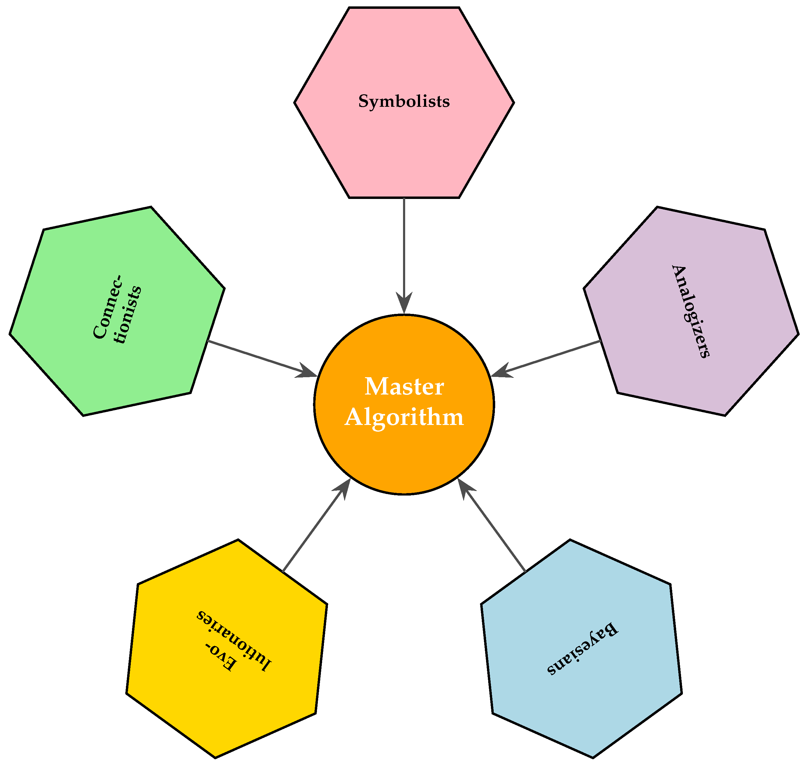
- Domingos, P. The master algorithm : how the quest for the ultimate learning machine will remake our world; Basic Books, A Member Of The Perseus Books Group: New York, 2015.
- Song, J.; Liu, Z.; Tegmark, M.; Gore, J. A Resource Model For Neural Scaling Law, 2024. [CrossRef]
- Radford, A.; Narasimhan, K.; Salimans, T.; Sutskever, I. Improving language understanding by generative pre-training, 2018.
- Alabdulmohsin, I.; Neyshabur, B.; Zhai, X. Revisiting Neural Scaling Laws in Language and Vision, 2022, [arXiv:cs.LG/2209.06640].
- Kaplan, J.; McCandlish, S.; Henighan, T.; Brown, T.B.; Chess, B.; Child, R.; Gray, S.; Radford, A.; Wu, J.; Amodei, D. Scaling Laws for Neural Language Models, 2020. [CrossRef]
- Hoffmann, J.; Borgeaud, S.; Mensch, A.; Buchatskaya, E.; Cai, T.; Rutherford, E.; de Las Casas, D.; Hendricks, L.A.; Welbl, J.; Clark, A.; et al. Training Compute-Optimal Large Language Models, 2022. [CrossRef]
- Besiroglu, T.; Erdil, E.; Barnett, M.; You, J. Chinchilla Scaling: A replication attempt, 2024. [CrossRef]
- Hutter, M. Learning Curve Theory, 2021. [CrossRef]
- Sharma, U.; Kaplan, J. A Neural Scaling Law from the Dimension of the Data Manifold, 2020. [CrossRef]
- Bahri, Y.; Dyer, E.; Kaplan, J.; Lee, J.; Sharma, U. Explaining neural scaling laws. Proceedings of the National Academy of Sciences 2024, 121. [CrossRef]
- Rosenfeld, J.S. Scaling Laws for Deep Learning. PhD thesis, Massachusetts Institute of Technology, Cambridge, MA, USA, 2021.
- Maloney, A.; Roberts, D.A.; Sully, J. A Solvable Model of Neural Scaling Laws, 2022. [CrossRef]
- Jeon, H.J.; Roy, B.V. Information-Theoretic Foundations for Neural Scaling Laws, 2024. [CrossRef]
- De Moura, L.; Bjørner, N. Z3: an efficient SMT solver. In Proceedings of the Proceedings of the Theory and Practice of Software, 14th International Conference on Tools and Algorithms for the Construction and Analysis of Systems, Berlin, Heidelberg, 2008; TACAS’08/ETAPS’08, p. 337–340.
- Vardi, G.; Yehudai, G.; Shamir, O. Width is Less Important than Depth in ReLU Neural Networks, 2022.
- Nguyen, T.; Raghu, M.; Kornblith, S. Do Wide and Deep Networks Learn the Same Things? Uncovering How Neural Network Representations Vary with Width and Depth, 2021. [CrossRef]
- Yu, M.; Wang, D.; Shan, Q.; Reed, C.J.; Wan, A. The Super Weight in Large Language Models, 2025. [CrossRef]
- Manoj, N.S.; Srebro, N. Interpolation Learning With Minimum Description Length, 2023. [CrossRef]
- Pitrat, J. A Step toward an Artificial Artificial Intelligence Scientist. Technical Report hal-03582345, LIP6, 2008.
- Bai, X.; Pres, I.; Deng, Y.; Tan, C.; Shieber, S.; Viégas, F.; Wattenberg, M.; Lee, A. Why Can’t Transformers Learn Multiplication? Reverse-Engineering Reveals Long-Range Dependency Pitfalls, 2025. [CrossRef]
- OpenAI. Preparedness Framework: Measuring and Managing Emerging Risks from Frontier Models, 2025. Accessed: 2025-11-26.
- Anthropic. Responsible Scaling Policy, Version 2.2, 2025. Accessed: 2025-11-26.
Disclaimer/Publisher’s Note: The statements, opinions and data contained in all publications are solely those of the individual author(s) and contributor(s) and not of MDPI and/or the editor(s). MDPI and/or the editor(s) disclaim responsibility for any injury to people or property resulting from any ideas, methods, instructions or products referred to in the content. |
© 2025 by the authors. Licensee MDPI, Basel, Switzerland. This article is an open access article distributed under the terms and conditions of the Creative Commons Attribution (CC BY) license (http://creativecommons.org/licenses/by/4.0/).


