
Submitted:
15 December 2025
Posted:
16 December 2025
You are already at the latest version
Abstract
The precise and automated classification of histopathology images is essential for early detection of cancer, particularly for widespread cancers like Colorectal Cancer (CRC) and Lung Cancer (LC). However, traditional deep learning models frequently encounter challenges due to significant intra-class variability, similarities between different classes, and inconsistent image quality. To overcome these limitations, a detailed multi-layer diagnostic framework is proposed. This method begins with a robust preprocessing pipeline that includes gamma correction, bilateral filtering, and adaptive CLAHE, leading to substantial improvements in quantitative metrics of image quality. A deep learning architecture based on hybrid attention mechanisms has been introduced, which integrates an Xception backbone, a Convolutional Block Attention Module (CBAM), a Transformer block, and an MLP classifier to effectively merge local features with global context. When evaluated on three publicly accessible datasets, the proposed model attained exemplary results, reaching classification accuracies of 99.98% on LC-2500, 99.58% on CRC-VAL-HE-7K, and 99.29% on NCT-CRC-HE-100K. To improve transparency, thorough explain ability analyses are performed utilizing layer-wise feature visualization and Grad-CAM. Lastly, the practical application of this framework is showcased through its implementation on a web-based platform, offering a valuable and user-friendly tool to assist in pathological diagnosis.
Keywords:
histopathology
; colorectal cancer
; lung cancer
; Xception
; CBAM
; image enhancement
; Grad-CAM
; deep learning
; web-based platform
1. Introduction
Cancer remains a significant cause of morality worldwide, with lung cancer and colorectal cancer (CRC) regularly ranking among the most common and deadly types [1]. The definitive diagnosis for most cancers, including CRC and lung cancer, relies on the histopathological examination of hematoxylin and eosin (H&E) stained tissue slides by expert pathologists [2]. Although this manual technique is regarded as the "gold standard," it is labor-intensive, subjective, and prone to considerable variability, both among different interpreters and within the same interpreter, which can negatively impact diagnostic reliability and patient outcomes [3]. To tackle these issues, the area of computational pathology has developed, utilizing computer-aided diagnosis (CAD) systems for more objective and efficient analyses. In the last decade, deep learning, particularly Convolutional Neural Networks (CNNs), has made significant progress in the classification of histopathological images [4]. Architectures such as ResNet, DenseNet, and Xception [5] have demonstrated their capability to retrieve intricate hierarchical features from pixel data, often achieving performance levels comparable to or even surpassing human capabilities in certain tasks. Nonetheless, these traditional CNN models confront two main limitations. Firstly, their convolutional architecture excels at detecting localized characteristics (for instance, the shape of cell nuclei) but frequently struggles to capture broader contextual details (such as the overall structure of the tissue), which is essential for precise diagnosis. Secondly, the "black box" nature of these models poses challenges for clinical application, as pathologists might find it difficult to comprehend the rationale behind the model's conclusions [6].
Moreover, the performance of any deep learning model heavily depends on the quality of the input data. Histopathological images exhibit considerable variability, frequently encountering problems related to stain intensity, variations in color, and artifacts arising from slide preparation [7]. Such variability can greatly diminish a model's ability to generalize effectively. While stain normalization is a common preprocessing step, simple normalization may not be sufficient. It is contended that a robust image enhancement pipeline is necessary not only to standardize images but also to reveal subtle textural details crucial for classification—a step that requires quantitative validation. To address these drawbacks, a new multi-stage hybrid deep learning framework is introduced. The process starts with a validated preprocessing pipeline that incorporates gamma correction, bilateral filtering, and Contrast Limited Adaptive Histogram Equalization (CLAHE) [8] to improve image quality. The metrics used to quantitatively assess these enhancements include Entropy and PSNR. For the classification task, a hybrid architecture is presented that utilizes the advantages of various paradigms. The Xception network [5] serves as a robust backbone for the extraction of local features. These features are subsequently refined through a Convolutional Block Attention Module (CBAM) [9], which adaptively readjusts the features by emphasizing the most significant spatial and channel-wise regions. To capture the wider context that traditional CNNs often miss, a Transformer block is integrated. Originally developed for natural language processing, Vision Transformers (ViT) [10] have demonstrated remarkable proficiency in capturing long-range dependencies within images, which makes them highly suitable for examining tissue architecture. The proposed model integrates these elements into a cohesive, end-to-end trainable network. To promote transparency and foster clinical confidence, explainability (XAI) techniques, particularly Gradient-weighted Class Activation Mapping (Grad-CAM) [11] and layer-wise feature visualization, are utilized to clarify the model's decisions. Ultimately, to showcase the practical applicability of this research, the trained model has been launched as an operational, web-based tool.
This model underwent extensive training and validation using three significant public datasets: NCT-CRC-HE-100K [12], CRC-VAL-HE-7K [12], and LC25000 [13]. The framework delivers state-of-the-art performance, showcasing a reliable, precise, and interpretable approach for automated histopathological diagnosis. The main contributions of this research are as follows:
- A quantitative comparison of histopathology images before and after a novel enhancement pipeline (gamma correction, bilateral filtering, CLAHE), using IQA metrics to validate its efficacy.
- The design and implementation of novel hybrid architecture (Xception-CBAM-Transformer) that synergistically combines local feature extraction, dual-axis attention, and global context modeling.
- State-of-the-art classification performance demonstrated on three distinct and widely used CRC and lung cancer datasets.
- A comprehensive explainability analysis using Grad-CAM and feature visualization to ensure model transparency and trustworthiness.
- The development and deployment of a web-based platform, translating our research into a practical tool for pathological assistance.
The following sections of this paper are structured as follows: Section 2 examines previous research relevant to the topic. Section 3 elaborates on the materials and methods, including an overview of the proposed framework and a description of the dataset. Section 4 outlines the experimental setup along with the implementation specifics. Section 5 delivers the experimental findings and offers an in-depth discussion. Lastly, Section 6 concludes with a summary of the findings.
2. Related Work
The automated examination of histopathological images for cancer classification has developed significantly, transitioning from conventional machine learning techniques to advanced deep learning frameworks. This section evaluates the main methods used for classifying colorectal cancer (CRC) and lung cancer, highlighting their respective strengths and weaknesses, which provides the rationale for the hybrid approach suggested in this paper.
2.1. Convolutional Neural Networks (CNNs) in Pathology
The first major advancement in computational pathology was the use of Convolutional Neural Networks (CNNs). Commonly utilized architectures that have been pre-trained on ImageNet, such as VGG [14], ResNet, and Xception [5], are frequently employed as feature extractors. Ongoing research continues to utilize these models, often in ensemble approaches, to attain high accuracy on datasets such as LC25000 and NCT-CRC-HE-100K [14,15].
Although these models excel at capturing local, hierarchical features (like nuclear atypia and mitotic figures), conventional CNNs have a key shortcoming: their effective receptive field is limited to a local scope. They find it challenging to represent long-range spatial relationships and the overall tissue architecture, such as the connections between tumor-infiltrating lymphocytes and epithelial cells that are distantly located, which are often vital for precise diagnosis and grading [16].
2.2. Attention-Enhanced CNNs
In order to overcome the shortcomings of conventional CNNs, researchers started incorporating attention mechanisms. These modules, such as the Convolutional Block Attention Module (CBAM) [9], help the network "learn what and where to emphasize." Recent 2024 studies confirm that integrating spatial and channel attention mechanisms (including CBAM) into CNN backbones significantly improves focus on critical regions, reduces noise, and enhances classification accuracy [17]. While these attention-gated CNNs improve performance, they are still fundamentally constrained by the convolutional backbone. They enhance the focus of local feature extraction but do not solve the problem of modeling global context.

Table 1.
Summary of Existing Models for Histopathological Image Classification.
| Model Category | Advantages | Limitations |
|---|---|---|
| Standard CNNs [5,14,15,20,50] | Excellent at extracting hierarchical local features (cell, nucleus morphology). Computationally efficient. | Limited effective receptive field fails to capture global tissue context. Highly sensitive to stain and color variations. |
| Attention-Enhanced CNNs [9,17,21] | Improves model focus on salient regions and suppresses background noise; enhances feature weighting across channels and space. | Still constrained by the CNN's local receptive field. Does not effectively model long-range dependencies. |
| Pure Transformers [10,18,22] | Excellent at modeling global context and long-range spatial relationships. | Requires massive training datasets. May lose fine-grained local texture details captured by CNNs. |
| Standard Hybrid Models [16,19,23] | Combines CNN local feature power with Transformer global context. (Represents current SOTA). | It can be overly complex. Often lacks a validated preprocessing stage and may not use fine-grained, low-level attention mechanisms (CBAM/SE). |
| Stain Invariance Networks [24,25] | Explicitly minimizes the variability caused by inconsistent H&E staining, improving generalization across different scanning centers. | Primary focus on color consistency may neglect morphological feature enhancement. Still reliant on local feature extractors. |
| Multiple Instance Learning (MIL) [26,27] | Handles extremely large Whole Slide Images (WSIs) by aggregating information from numerous small patches. Often includes a form of patch-level attention. | Aggregation layer may lose crucial spatial relationships between patches. Computationally intensive due to sequential tile processing. |
| Proposed Model (Enhancement + Xception-CBAM-Transformer) |
Designed to solve all listed limitations: (1) Preprocessing handles stain variance. (2) Xception captures local detail. (3) CBAM refines feature focus. (4) Transformer models global context. | - |
2.3. Transformers in Computational Pathology
Recently, the Vision Transformer (ViT) [10] has emerged as a formidable alternative. According to a comprehensive analysis by Xu et al. [18] released in 2024, the application of Transformers is increasingly prevalent in the domain of pathology. They effectively understand global, long-range relationships by dividing an image into smaller segments and employing self-attention. Nonetheless, pure Transformers are known for their substantial data requirements and may miss the detailed, pixel-level textural details that CNNs excel in capturing.
2.4. Hybrid Architectures and Identified Gaps
The latest advancements are leaning towards hybrid models that integrate the advantages of both frameworks: employing a CNN for effective local feature extraction and a Transformer to capture the overarching context of these features. Recent research in 2024 has clearly shown the effectiveness of hybrid Xception-Transformer architectures, confirming the strategy of utilizing Xception for enhancing local features that are then processed by a Transformer for modeling global context [19].
This is precisely where our work is positioned, but with key improvements. We identify three critical gaps in existing literature:
- Preprocessing: Many studies do not employ or, more importantly, quantitatively validate a preprocessing pipeline to handle the extreme stain variability in multi-center datasets.
- Feature Refinement: While hybrid models exist [19], the features are often passed directly from the CNN to the Transformer. We hypothesize that first refining these features with a lightweight dual-attention mechanism (CBAM) provides a more salient and robust input to the Transformer block.
- Explainability: Many complex hybrid models remain "black boxes." We integrate Grad-CAM and feature visualization as a core part of our methodology to ensure clinical trust and interpretability.
The proposed model validated preprocessing pipeline followed by an Xception-CBAM-Transformer network—is explicitly designed to address these three gaps. The following table summarizes the key models and their limitations, which our approach aims to resolve.
3. Materials and Methods
This section details the datasets, preprocessing pipeline, and the novel hybrid architecture used in this study. The overall workflow of our methodology is presented in Figure 1.
3.1. Dataset Description
We utilized three publicly available, large-scale histopathology datasets to ensure the robustness and generalizability of our model.
- CRC-VAL-HE-7K [12]: This validation set is associated with the NCT-CRC dataset and comprises 7,180 image patches from various patients, providing a strong evaluation of the model's ability to generalize.
- NCT-CRC-HE-100K [12]: This dataset comprises 100,000 distinct image patches derived from 86 patients. Each image has dimensions of 224x224 pixels and features nine different tissue categories: Adipose (ADI), Background (BACK), Debris (DEB), Lymphocytes (LYM), Mucus (MUC), Smooth Muscle (MUS), Normal Colon Mucosa (NORM), Cancer-Associated Stroma (STR), and Colorectal Adenocarcinoma Epithelium (TUM).
- LC25000 [13]: This dataset on "Lung and Colon Cancer" comprises 25,000 colored images (768x768 pixels) that are categorized into five classes: three types of lung tissue (Lung Adenocarcinoma, Lung Squamous Carcinoma, Benign Lung Tissue) and two types of colon tissue (Colon Adenocarcinoma, Benign Colon Tissue).
The visualization of the CRC-VAL-HE-7k, NCT-CRC-HE-100k, LC-2500 datasets class distribution is shown in Figure 2.
3.2. Image Preprocessing and Enhancement
Histopathological images often show considerable variability in staining and appearance. To unify the data and amplify important features, we developed a multi-phase preprocessing pipeline.
3.2.1. Image Enhancement
This initial phase, applied before the train/validation split, aimed to improve image fidelity.
- Gamma Correction: Gamma correction modifies the general brightness and contrast of an image through a nonlinear transformation, enhancing the visibility of both dark and light areas.where is the original pixel intensity at coordinates (x, y), is the gamma-corrected intensity, and γ is the correction parameter. In this study, γ = 1.2 was selected to enhance contrast without overexposure.
- Bilateral Filtering: Bilateral filtering minimizes noise while retaining edges, which is crucial for preserving the structural details of nuclei and tissues in histopathology images. The output of the bilateral filter at the pixel (x, y) is calculated in the following manner:where Ω is the spatial neighborhood around pixel (), controls spatial smoothing, controls intensity similarity, and Wp is the normalization factor.
- Adaptive CLAHE: Bilateral Adaptive Contrast Limited Histogram Equalization (CLAHE) enhances local contrast while preventing over-amplification of noise in homogeneous regions. For each pixel (x, y) in each tile, the output intensity is computed as:where is the clipped cumulative distribution function of the pixel intesities 149 within the tile, and L is the total number of possible intensity levels (typically 256). Clipping 150 limits the slope of the CDF, preventing over-enhancement in nearly uniform regions.
The overall image enhancement workflow is illustrated in Figure 3, which outlines the sequential application of gamma correction, bilateral filtering, and CLAHE to improve the contrast and structural clarity of histopathological images. Initially, brightness and contrast were adjusted using gamma correction (γ = 1.2), which brought out fine details in the darkest zones. Subsequently, a bilateral filter was applied to decrease noise while maintaining tissue and tumor edges. Finally, Contrast Limited Adaptive Histogram Equalization (CLAHE), applied in the LAB color space, enhanced local contrast and emphasized fine structural details.
This sequence produced enhanced images with better visual quality and preserved structural integrity, making them more appropriate for downstream classification tasks. The enhanced images according to their classes are represented in Figure 4.
Tables 5–10 present the image quality assessment results for the original and enhanced images across the CRC-VAL-HE-7k, NCT-CRC-HE-100K, and LC25000 datasets. For the CRC-VAL-HE-7k dataset (Tables 5 and 6), the original images exhibit class-dependent variations in entropy and sharpness, with classes such as NORM, LYM, and STR showing higher entropy and SI values, indicating richer structural information.
Table 5 presents the average image quality metrics for each class of the original images on CRC-VAL-HE-7k dataset.
| Class | Entropy | SI | PSNR (db) | IQI |
| ADI | 5.3087 | 13.5822 | 100.00 | 1.0 |
| BACK | 3.9238 | 4.9472 | 100.00 | 1.0 |
| DEB | 6.8641 | 18.8359 | 100.00 | 1.0 |
| LYM | 7.3665 | 24.9039 | 100.00 | 1.0 |
| MUC | 6.9295 | 20.7820 | 100.00 | 1.0 |
| MUS | 6.8906 | 17.7147 | 100.00 | 1.0 |
| NORM | 7.4485 | 17.6426 | 100.00 | 1.0 |
| STR | 7.0325 | 19.4184 | 100.00 | 1.0 |
| TUM | 7.1196 | 15.6653 | 100.00 | 1.0 |
Table 6 presents the average image quality metrics for each class of enhanced images on CRC-VAL-HE-7k dataset.
| Class | Entropy | SI | PSNR (db) | IQI |
| ADI | 5.9625 | 14.0326 | 26.9067 | 0.9943 |
| BACK | 5.1629 | 4.6107 | 18.8282 | 0.9316 |
| DEB | 7.4049 | 21.5364 | 21.9243 | 0.9744 |
| LYM | 7.7233 | 29.3981 | 21.9710 | 0.9750 |
| MUC | 7.3384 | 20.7820 | 23.4738 | 0.9814 |
| MUS | 7.3787 | 19.8815 | 22.2676 | 0.9813 |
| NORM | 7.7302 | 20.4912 | 21.9938 | 0.9749 |
| STR | 7.4978 | 22.5964 | 21.1507 | 0.9762 |
| TUM | 7.5359 | 17.6582 | 21.7172 | 0.9762 |
All original images maintain the maximum PSNR (100 dB) and IQI (1.0). After enhancement, entropy and SI increase consistently across all classes, confirming improved textural details, while PSNR and IQI slightly decrease as expected due to the introduction of new high-frequency information during enhancement.
A similar trend is observed in the NCT-CRC-HE-100K dataset (Tables 7 and 8).
Table 7 presents the average image quality metrics for each class of the original images on NCT-CRC-100k dataset.
| Class | Entropy | SI | PSNR (db) | IQI |
| ADI | 5.1162 | 16.2056 | 100.00 | 1.0 |
| BACK | 3.7543 | 4.9802 | 100.00 | 1.0 |
| DEB | 6.7772 | 19.1007 | 100.00 | 1.0 |
| LYM | 7.3677 | 21.6227 | 100.00 | 1.0 |
| MUC | 7.0829 | 17.7169 | 100.00 | 1.0 |
| MUS | 6.8061 | 18.9369 | 100.00 | 1.0 |
| NORM | 7.3585 | 19.1077 | 100.00 | 1.0 |
| STR | 6.9971 | 20.0641 | 100.00 | 1.0 |
| TUM | 7.1653 | 20.4176 | 100.00 | 1.0 |
Table 8 presents the average image quality metrics for each class of enhanced images on NCT-CRC-100k dataset.
| Class | Entropy | SI | PSNR (db) | IQI |
| ADI | 5.7392 | 16.4826 | 26.8352 | 0.9960 |
| BACK | 5.0444 | 4.6428 | 22.3114 | 0.9522 |
| DEB | 7.2333 | 21.5301 | 22.8247 | 0.9813 |
| LYM | 7.7413 | 27.3297 | 22.0819 | 0.9744 |
| MUC | 7.4602 | 19.4021 | 22.5264 | 0.9827 |
| MUS | 7.2743 | 21.3647 | 22.6810 | 0.9833 |
| NORM | 7.6924 | 22.1051 | 22.0992 | 0.9773 |
| STR | 7.4583 | 23.2537 | 22.1608 | 0.9812 |
| TUM | 7.5758 | 23.6460 | 21.9519 | 0.9793 |
The original images again show uniformly high PSNR and IQI values, whereas the enhanced images demonstrate increased entropy and SI across all classes, signifying improved visual sharpness and contrast. Although PSNR values decrease from the ideal 100 dB to the 21–27 dB range, the IQI values remain high (0.95–0.99), indicating preservation of structural similarity.
For the LC25000 dataset (Tables 9 and 10), the same pattern is maintained. Original images yield perfect PSNR and IQI values, while enhancement results in higher entropy and SI, particularly in colon_aca and colon_bnt, reflecting significant texture amplification. The enhanced PSNR values fall within the expected range (16–21 dB), with IQI values consistently above 0.93, demonstrating that the enhancement improves detail while preserving structural integrity.
Table 9 presents the average image quality metrics for each class of the original images on LC-2500 dataset.
| Class | Entropy | SI | PSNR (db) | IQI |
| colon_aca | 7.0919 | 28.2666 | 100.00 | 1.0 |
| colon_bnt | 7.1505 | 28.0476 | 100.00 | 1.0 |
| lung_aca | 7.0451 | 14.2314 | 100.00 | 1.0 |
| Lung_bnt | 6.6160 | 13.7855 | 100.00 | 1.0 |
| Lung_scc | 6.7575 | 13.9977 | 100.00 | 1.0 |
Table 10 presents the average image quality metrics for each class of enhanced images on LC-2500 dataset.
| Class | Entropy | SI | PSNR (db) | IQI |
| colon_aca | 7.6567 | 34.2878 | 17.2238 | 0.9511 |
| colon_bnt | 7.7199 | 32.7993 | 16.1384 | 0.9375 |
| lung_aca | 7.5795 | 19.8720 | 21.1361 | 0.9680 |
| Lung_bnt | 7.2235 | 18.2911 | 21.6530 | 0.9780 |
| Lung_scc | 7.4720 | 20.4731 | 20.7948 | 0.9687 |
Overall, the quantitative results across all three datasets confirm that the proposed enhancement method increases image entropy and sharpness while maintaining high structural quality, ensuring improved visual and textural richness suitable for downstream deep learning tasks.
3.3. Baseline Models for Comparison
Training deep learning models on large datasets is essential to avoid overfitting. Transfer learning allows for effective training with smaller, specialized datasets by refining pre-trained models, which boosts performance and reduces training time. To benchmark our proposed model, we implemented and fine-tuned several advanced CNN architectures known for their potent image recognition performance. We fine-tuned these models on our enhanced histopathology datasets to compare their ability to classify CRC and Lung Cancer.
- DenseNet121: Introduced by Huang et al. [28], this model utilizes dense skip connections to improve feature reuse, decrease parameters, and improve gradient flow.
- MobileNetV2: Sandler et al. [29] introduced an architecture that employs inverted residuals and linear bottlenecks (depthwise separable convolutions) to reduce computational cost, making it highly efficient.
- NASNetMobile: Zoph et al. [30] used neural architecture search to identify an effective network structure optimized for high performance on mobile-sized models.
- InceptionV3: Szegedy et al. [31] use factorized convolutions to enhance efficiency by reducing connections without sacrificing performance, and it is known for its multi-scale processing.
- VGG16: Introduced by Simonyan and Zisserman [32], this 16-layer model is renowned for its simplicity and uniform 3x3 filter-based architecture.
- Xception: Chollet [5] improved the Inception architecture by replacing Inception modules with depthwise separable convolutions and adding residual connections, achieving high accuracy with fewer parameters.
3.4. Proposed Hybrid Architecture
The proposed model, illustrated in Figure 5, represents an innovative hybrid structure. It aims to recognize both local morphological characteristics and global contextual relationships.
3.4.1. Xception Backbone (Local Feature Extractor)
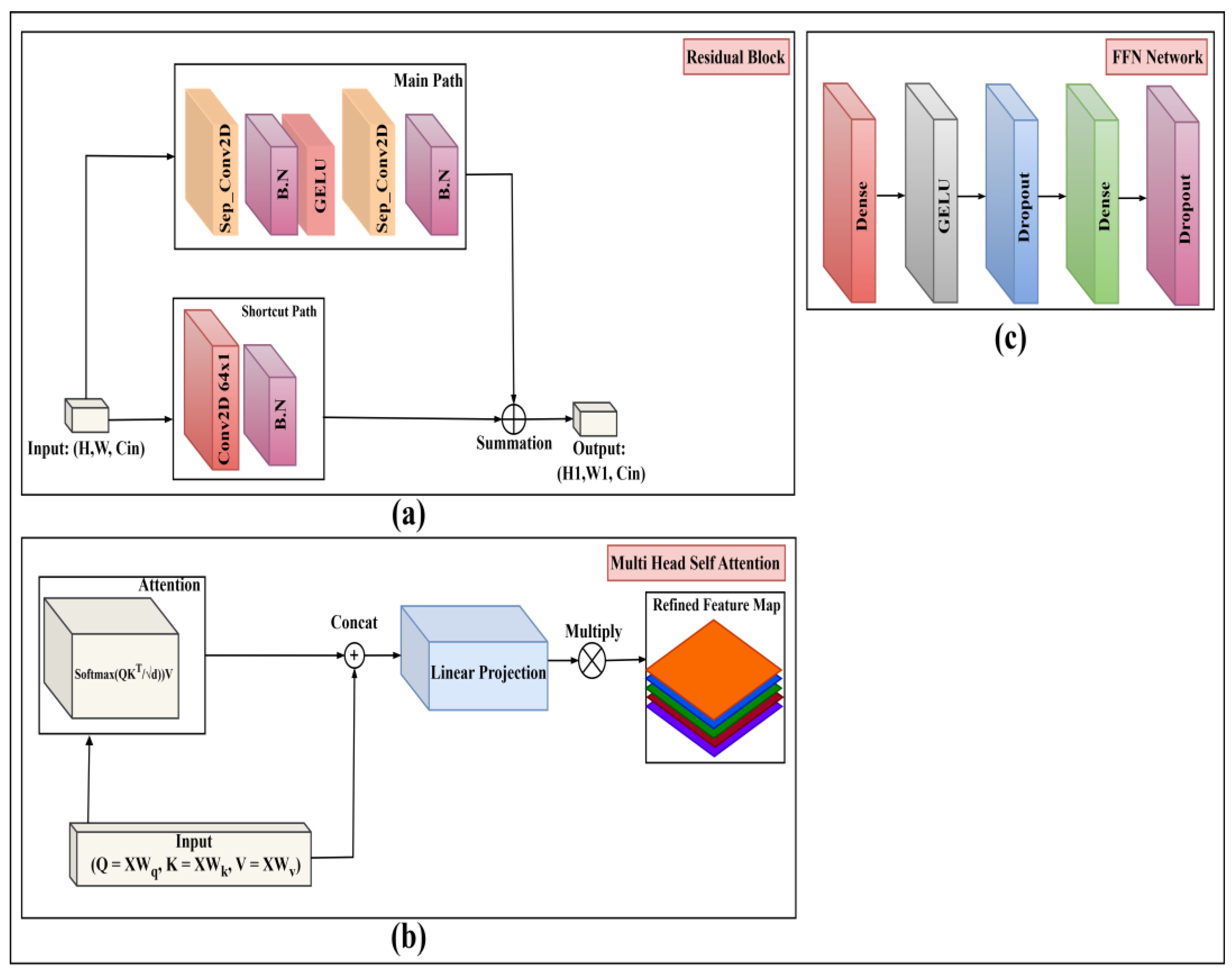
The 224x224x1 preprocessed images serve as input to the Xception Block (Figure 5a). We use the Xception architecture [5] as our primary local feature extractor. This backbone is built upon a series of Residual Blocks as detailed in Figure 6a. Each block consists of a 'Main Path' and a 'Shortcut Path'.
- Main Path: The input passes through a Separable 2D Convolution (Sep_Conv2D), Batch Normalization (BN), a GeLU activation, another Sep_Conv2D, and a final BN.
- Shortcut Path: The original input is passed through a 1x1 Convolution (Conv2D 64x1) and a BN layer to match the channel dimensions of the main path.
3.4.2. CBAM Attention (Feature Refinement)
The high-level feature map from the Xception backbone is immediately passed to the CBAM Block (Figure 5b) for feature refinement. This module [9] sequentially infers and applies channel and spatial attention maps to recalibrate the feature map, amplifying salient information and suppressing irrelevant noise before it is passed to the Transformer.
3.4.3. Transformer Encoder (Global Context Modeling)
To model global context, the refined feature map from CBAM is "tokenized" (flattened into a 1D sequence of feature vectors) and combined with a learned positional embedding. This sequence is fed into the Transformer Block (Figure. 5c). This block follows the standard encoder architecture [10], which is composed of two primary sub-layers:
- Multi-Head Self-Attention (MHSA): As detailed in Figure 6b, the input sequence (X) is used to generate the Query (Q), Key (K), and Value (V) matrices through learned linear projections. The attention output is calculated using scaled dot-product attention: Attention = Softmax. The outputs from multiple such "heads" are concatenated, passed through a final linear projection, and multiplied to produce the refined feature map. This allows the model to weigh the importance of every feature token relative to every other token.
- Feed-Forward Network (FFN): As shown in Figure 6c, the output of the MHSA sub-layer is passed through a position-wise FFN. This network consists of two Dense (fully connected) layers separated by a GeLU activation and Dropout layers for regularization.
Residual connections and layer normalization are applied around each of these two sub-layers (MHSA and FFN) as shown in Figure 5c.
Figure 5.
Overall architecture of the proposed hybrid model. (a) Xception backbone for hierarchical feature extraction, (b) Convolutional Block Attention Module (CBAM) for spatial–channel attention refinement, (c) Transformer block for capturing long-range spatial dependencies and, (d) Classification head for final prediction across all target classes.
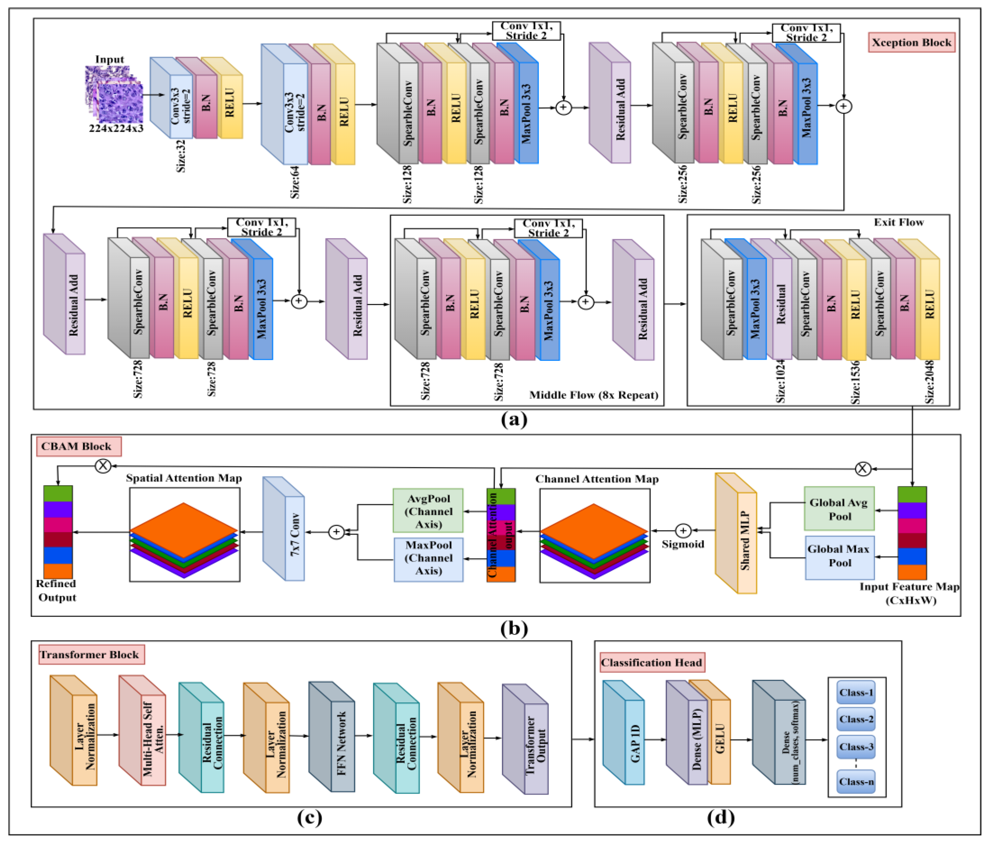
3.4.4. Classification Head
The output sequence from the Transformer block is processed by the final Classification Head (Figure 5d). First, a Global Average Pooling 1D (GAP1D) layer is applied to condense the token sequence into a single, fixed-size feature vector. This vector is then passed through a small MLP, consisting of a Dense (FC) layer with a ReLU activation, followed by the final Dense (FC) layer with a Softmax activation to produce a probability distribution across the n output classes.
Figure 6.
Proposed Model Architecture with Attention: (a) Residual block, (b) Multiheaded self-attention (c) FFN network.
Figure 6.
Proposed Model Architecture with Attention: (a) Residual block, (b) Multiheaded self-attention (c) FFN network.
3.5. Web-Based Deployment
To demonstrate translational applicability, the final, optimized model was deployed as an interactive, web-based tool where a user can upload a histopathology image and receive a classification.
4. Experimental Setup
This segment describes the technical details of the hardware utilized for training and the hyperparameter configurations employed across all models.
4.1. Hardware Configuration
All experiments were conducted on a workstation with the specifications detailed in Table 11. The deep learning models were created, trained, and evaluated using the TensorFlow and Keras libraries (version 2.10) in conjunction with Python 3.9 [51].
| Hardware Specifications | Details |
| Platform | Jupyter Notebook |
| Processor | AMD Ryzen 5 3600 |
| Memory (RAM) | 16GB |
| Operating System | Ubuntu 23.10, 64 bit |
| Graphics Card | Nvidia GeForce GTX 1660 (VRAM 6GB) |
4.2. Hyperparameter Settings
The model was trained on 224 × 224 × 3 inputs for 100 epochs with a batch size of 8 using the Adam optimizer (learning rate 1 × 10⁻⁴) and categorical cross-entropy loss. A dropout rate of 0.5 was applied before the SoftMax layer to decrease overfitting. A 20% validation split was used for data augmentation, which includes rescaling, shearing, zooming, rotating, width/height shifts, horizontal flips, and brightness modifications. The architecture consists of five residual blocks, each featuring SeparableConv2D and batch normalization, followed by global average pooling and a five-class SoftMax head. The best checkpoint was saved automatically based on validation performance. All hyperparameter settings used in the training process are summarized in Table V.
Table 12.
Hyperparameters used in training the Proposed Model.
| Hyperparameter | Value |
|---|---|
| Input image size | 224 × 224 × 3 |
| Number of classes | 5, 9 & 9 |
| Batch size | 16 |
| Number of epochs | 50,100 & 100 |
| Optimizer | Adam |
| Learning rate | 1 × 10⁻⁴ |
| Loss function | Categorical Cross entropy |
| Dropout rate | 0.5 |
| Data augmentation | Rescale (1/255), Shear (0.3), Zoom (0.3), Rotation (30◦), Width shift (0.2), Height shift (0.2), Horizontal flip, Brightness range [0.7, 1.3] |
| Model architecture | Xception Backbone, CBAM Attention Layer, and Transformer block |
| Pooling layer | Global Average Pooling |
| Final activation | Softmax |
| Callback | ModelCheckpoint (save best) |
5. Result Analysis and Discussion
This segment offers an in-depth evaluation of the experimental findings. We first define the performance metrics used, then present the detailed performance of our proposed model, and finally compare it against the baseline models and existing state-of-the-art research.
5.1. Performance Metrics
Metrics of evaluation are crucial for assessing the performance of the model. Accuracy, Precision, Sensitivity, F1- score, AUC, Loss, Cohen’s Kappa, and Matthews Correlation Coefficient (MCC) were among the metrics we utilized to evaluate our classification model. Here in this context, TP, TN, FP, and FN stand for True Positives, True Negatives, False Positives, and False Negatives, respectively [52,53,54].
Where, is observed agreement (accuracy) and is expected agreement.
5.2. Performance Results
In this subsection, we analyze the quantitative and qualitative performance of the proposed hybrid model.
5.2.1. Confusion Matrices
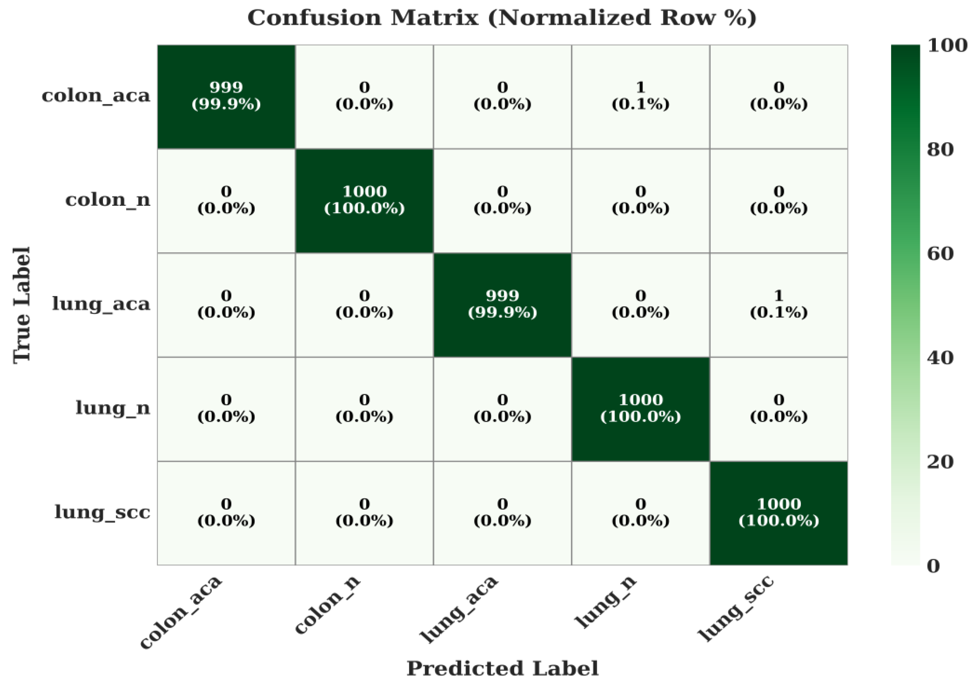
The class-wise performance of the proposed model is detailed in the normalized confusion matrices in Figure 7, Figure 8 and Figure 9.
The model achieves exceptional accuracy, with most classes at or near 100%. For instance, ADI, BACK, DEB, LYM, and STR are all classified with >99.6% accuracy. The most complex class, TUM (Tumor), is still correctly identified 98.8% of the time, with only minor, clinically expected confusion with related tissues like NORM (0.8%).
Figure 7.
Confusion Matrix of the Proposed Model on CRC-VAL-HE-7k Dataset.
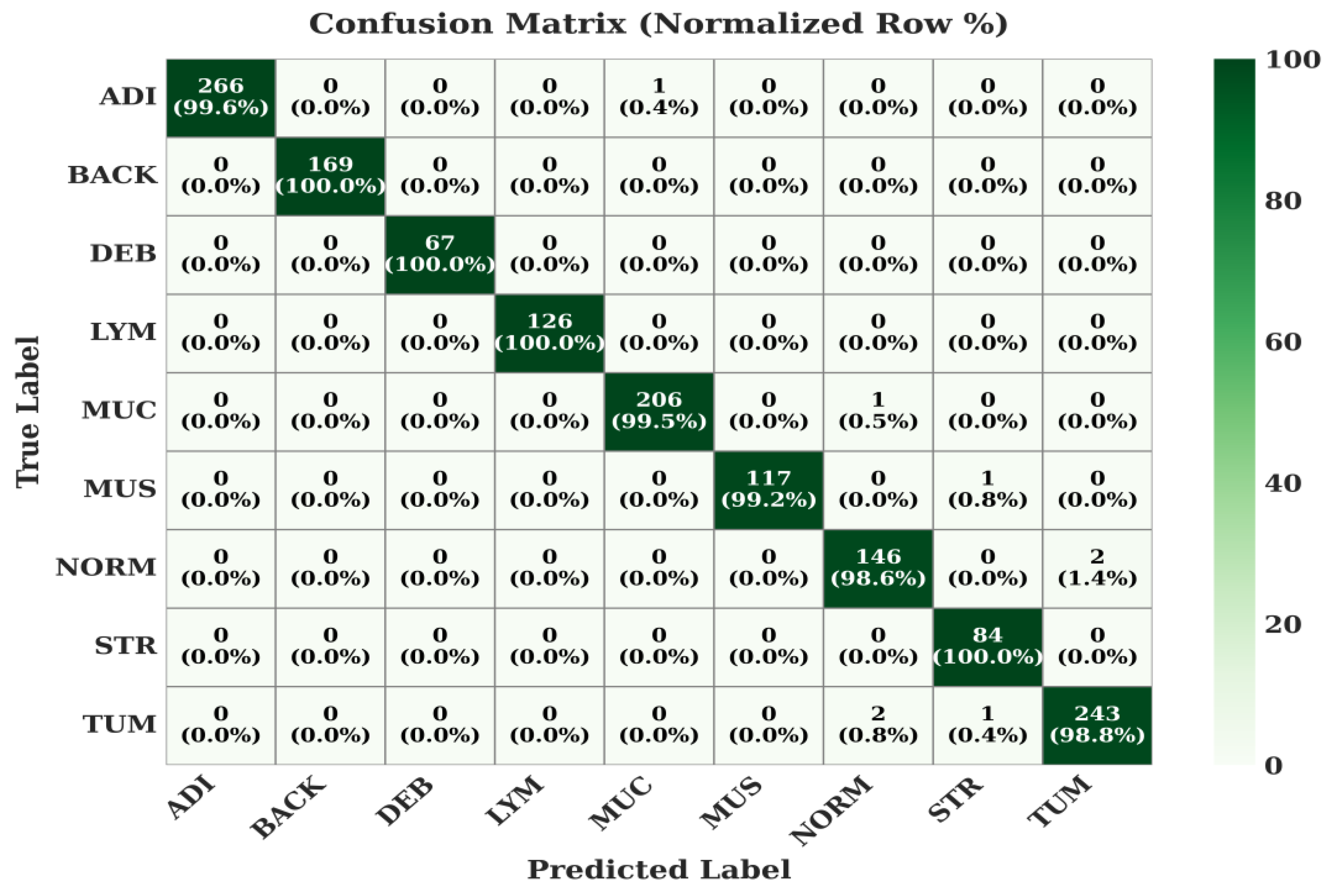
On this larger and more complex 9-class dataset, the model's robustness is evident. It achieves 100% for ADI and LYM. The TUM (Tumor) class, which is notoriously difficult, is correctly classified 98.6% of the time, with slight confusion with other stromal and mucosal classes (MUC, NORM, STR), which is a common challenge in pathology.
Figure 8.
Confusion Matrix of the Proposed Model on NCT-CRC-HE-100k Dataset.

The model's performance on the 5-class lung and colon dataset is virtually flawless. colon_n, lung_n, and lung_scc are all classified with 100% accuracy. The adenocarcinoma classes (colon_aca, lung_aca) are classified with 99.9% accuracy, demonstrating the model's profound capability to distinguish between benign and malignant tissues, as well as between different types of carcinomas.
Figure 9.
Confusion Matrix of the Proposed Model on LC-2500 Dataset.
5.2.2. Training and Validation
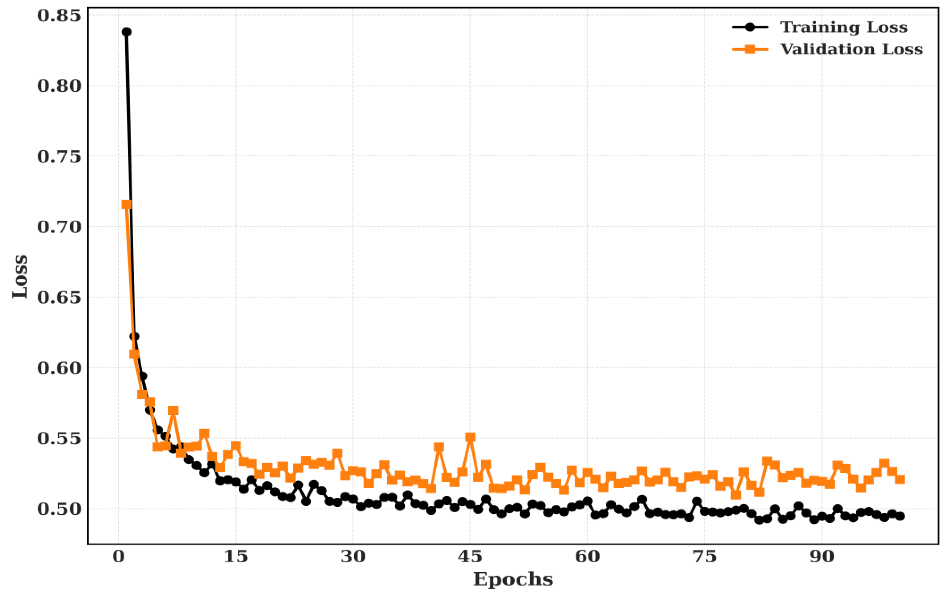
The Training and Validation Accuracy and Training and validation loss for CRC-VAL-HE-7k dataset is shown in Figure 9 and Figure 10.
Figure 10.
The proposed model’s training and validation accuracy for CRC-VAL-7k.
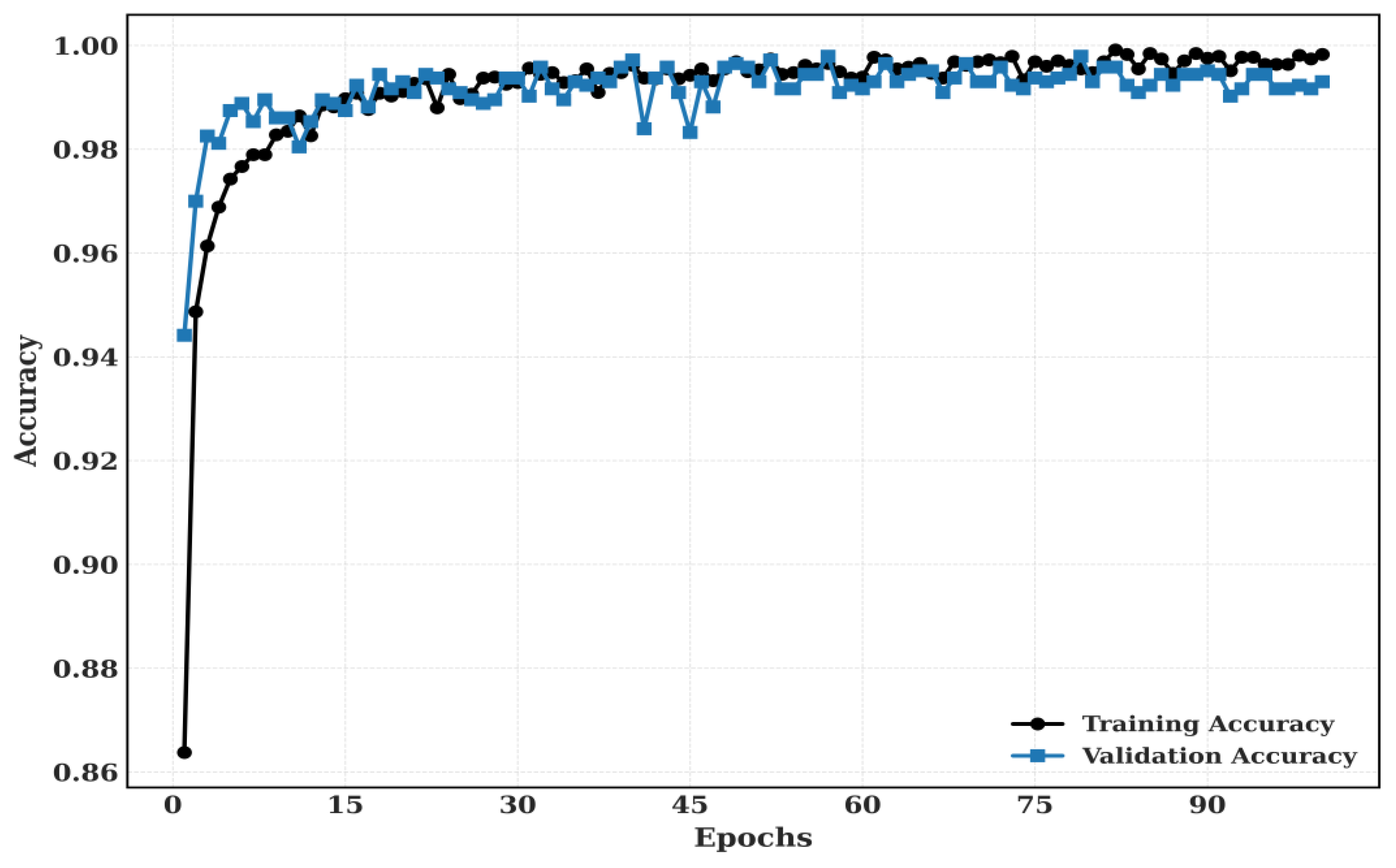
Figure 11.
The proposed model’s training and validation loss for CRC-VAL-7k.
5.2.3. Feature Space and ROC Analysis
The discriminative power of the learned features is visualized in Figure 16, Figure 17 and Figure 18 using t-SNE. These plots show clear, well-separated clusters for the different tissue classes.
The model's superiority is benchmarked in the ROC curves in Figure 19, Figure 20 and Figure 21. These figures compare the Area Under the Curve (AUC) of our proposed model against all six baselines (InceptionV3, NASNetMobile, VGG16, Xception, DenseNet121, MobileNetV2) for the three datasets. Our model consistently achieves the highest AUC, approaching 1.0.
5.2.4. Explainability Visualization
5.3. Comparative Analysis
In this section, the performance of the proposed model is evaluated against pretrained deep learning baselines and existing work reported in the literature, with per-class performance metrics provided.
Table 13.
Comparative performance of pretrained models and the proposed model on CRC-VAL-HE-7k.
| Model | Accuracy | Precision | Recall | F1-score | MCC | Kappa |
|---|---|---|---|---|---|---|
| Densenet-121 | 99.58 | 99.60 | 99.60 | 99.60 | 99.58 | 99.57 |
| MobileNetV2 | 97.76 | 96.73 | 96.89 | 96.81 | 96.60 | 96.61 |
| Xception | 99.20 | 98.77 | 98.84 | 98.80 | 98.78 | 98.79 |
| InceptionV3 | 97.27 | 97.14 | 97.89 | 96.38 | 96.63 | 95.82 |
| VGG-16 | 98.18 | 97.54 | 96.70 | 97.12 | 97.08 | 97.09 |
| NasNetMobile | 94.35 | 95.08 | 93.30 | 94.19 | 98.32 | 93.86 |
| Proposed Model | 99.58 | 99.10 | 99.00 | 99.40 | 99.40 | 99.40 |
Table 14.
Per-Class Performance Metrics for Each Histopathological Class on CRC-VAL-HE-7k.
| Class | Precision | Recall | F1-Score | Per-Class Acc. | MCC | Support |
|---|---|---|---|---|---|---|
| ADI | 1.0000 | 0.9925 | 0.9962 | 0.9986 | 0.9954 | 267 |
| BACK | 1.0000 | 1.0000 | 1.0000 | 1.0000 | 1.0000 | 169 |
| DEB | 1.0000 | 0.9851 | 0.9925 | 0.9993 | 0.9921 | 67 |
| LYM | 1.0000 | 0.9921 | 0.9960 | 0.9993 | 0.9956 | 126 |
| MUC | 1.0000 | 0.9952 | 0.9976 | 0.9993 | 0.9972 | 207 |
| MUS | 1.0000 | 0.9831 | 0.9915 | 0.9986 | 0.9907 | 118 |
| NORM | 1.0000 | 0.9932 | 0.9966 | 0.9993 | 0.9962 | 148 |
| STR | 0.9545 | 1.0000 | 0.9767 | 0.9972 | 0.9756 | 84 |
| TUM | 0.9840 | 1.0000 | 0.9919 | 0.9972 | 0.9903 | 246 |
| Macro Avg | 0.9932 | 0.9935 | 0.9932 | 0.9988 | 0.9926 | – |
| Weighted Avg | 0.9946 | 0.9944 | 0.9944 | 0.9987 | 0.9937 | 1432 |
Table 15.
Comparative performance of pretrained models and the proposed model on NCT-CRC-HE-100k.
| Model | Accuracy | Precision | Recall | F1-score | MCC | Kappa |
|---|---|---|---|---|---|---|
| Densenet-121 | 96.81 | 96.81 | 96.81 | 96.81 | 96.40 | 96.40 |
| MobileNetV2 | 96.30 | 96.25 | 96.29 | 96.29 | 95.83 | 95.82 |
| Xception | 98.16 | 98.12 | 98.18 | 98.14 | 97.92 | 97.92 |
| InceptionV3 | 95.20 | 95.17 | 95.13 | 95.14 | 94.58 | 94.58 |
| VGG-16 | 97.02 | 96.94 | 97.06 | 96.98 | 96.65 | 96.64 |
| NasNetMobile | 94.20 | 94.16 | 94.10 | 94.12 | 93.46 | 93.45 |
| Proposed Model | 99.29 | 99.32 | 99.26 | 99.29 | 99.21 | 99.20 |
Table 16.
Per-Class Performance Metrics for Each Histopathological Class on on NCT-CRC-HE-100k.
| Class | Precision | Recall | F1-Score | Per-Class Acc. | MCC | Support |
|---|---|---|---|---|---|---|
| ADI | 0.9981 | 0.9981 | 0.9981 | 0.9996 | 0.9979 | 2081 |
| BACK | 0.9991 | 0.9986 | 0.9988 | 0.9997 | 0.9987 | 2113 |
| DEB | 0.9858 | 0.9952 | 0.9905 | 0.9978 | 0.9893 | 2302 |
| LYM | 0.9996 | 0.9944 | 0.9970 | 0.9993 | 0.9966 | 2311 |
| MUC | 0.9977 | 0.9826 | 0.9901 | 0.9982 | 0.9892 | 1779 |
| MUS | 0.9937 | 0.9948 | 0.9943 | 0.9984 | 0.9934 | 2707 |
| NORM | 0.9897 | 0.9897 | 0.9897 | 0.9982 | 0.9887 | 1752 |
| STR | 0.9871 | 0.9885 | 0.9878 | 0.9974 | 0.9864 | 2089 |
| TUM | 0.9882 | 0.9923 | 0.9902 | 0.9972 | 0.9886 | 2863 |
| Macro Avg | 0.9932 | 0.9927 | 0.9929 | 0.9984 | 0.9921 | – |
| Weighted Avg | 0.9930 | 0.9930 | 0.9930 | 0.9984 | 0.9921 | 19997 |
Table 17.
Comparative performance of pretrained models and the proposed model on LC25000 dataset.
| Model | Accuracy | Precision | Recall | F1-score | MCC | Kappa |
|---|---|---|---|---|---|---|
| Densenet-121 | 99.26 | 99.52 | 99.52 | 99.52 | 99.40 | 99.25 |
| MobileNetV2 | 99.26 | 99.37 | 99.38 | 99.37 | 99.25 | 99.20 |
| Xception | 99.68 | 99.68 | 99.68 | 99.68 | 99.60 | 99.42 |
| InceptionV3 | 97.86 | 97.88 | 97.84 | 97.83 | 97.31 | 97.32 |
| VGG-16 | 99.72 | 99.78 | 99.78 | 99.78 | 99.72 | 99.60 |
| NasNetMobile | 97.74 | 97.82 | 97.78 | 97.78 | 97.32 | 97.45 |
| Proposed Model | 99.98 | 99.98 | 99.98 | 99.98 | 99.75 | 99.75 |
Table 18.
Per-Class Performance Metrics for Colon and Lung Cancer Classification on LC-2500 dataset.
Table 18.
Per-Class Performance Metrics for Colon and Lung Cancer Classification on LC-2500 dataset.
| Class | Precision | Recall | F1-score | Per-class Acc. | MCC | Support |
|---|---|---|---|---|---|---|
| colon_aca | 1.0000 | 1.0000 | 1.0000 | 1.0000 | 1.0000 | 1000 |
| colon_bnt | 1.0000 | 1.0000 | 1.0000 | 1.0000 | 1.0000 | 1000 |
| lung_aca | 0.9990 | 1.0000 | 0.9995 | 0.9996 | 0.9988 | 1000 |
| lung_bnt | 1.0000 | 1.0000 | 1.0000 | 1.0000 | 1.0000 | 1000 |
| lung_scc | 1.0000 | 0.9990 | 0.9996 | 0.9996 | 0.9987 | 1000 |
| Macro Avg | 0.9998 | 0.9998 | 0.9998 | 0.9998 | 0.9995 | – |
| Weighted Avg | 0.9998 | 0.9998 | 0.9998 | 0.9998 | 0.9995 | 5000 |
Table 19.
Step by step implementation approaches of the proposed model on LC-2500 dataset.
| Model Variant | Params | FLOPS (G) | Inference (ms) | Accuracy (%) | F1 (%) | Acc Vs Base (%) |
|---|---|---|---|---|---|---|
| Ensemble (MobilenetV2 + Xception + VGG16) | 164.8M | 24.2 | 112 | 98.76 0.21 | 96.74 0.23 | 3.24 |
| Xception (ImageNet) | 21.9M | 4.2G | 7.66 | 99.68 0.17 | 99.68 0.26 | 0.30 |
| Xception Conv5 | 7.6M | 3.8G | 3.6 | 97.58 0.38 | 97.48 0.62 | 2.20 |
| Xception + Spatial Attention | 0.66M | 1.5G | 0.7 | 98.54 0.04 | 98.38 0.34 | 1.11 |
| Xception (like-CNN) + SE + CBAM | 3.01M | 2.45G | 11.3 | 98.53 0.15 | 98.46 0.36 | 1.45 |
| Xception + CBAM Attention + Transformer | 20.1M | 3.9G | 7.1 | 99.980.01 | 99.980.01 |
Table 20.
Performance Comparison Between Prior Work and the Proposed Model on LC2500 dataset.
| Model | Dataset | Accuracy | Precision | Recall | F1-Score | MCC | Kappa | Ref. |
|---|---|---|---|---|---|---|---|---|
| Fine-tuned ResNet101 | LC2500 | 99.94 | 99.84 | 99.85 | 99.84 | NA | NA | [33] |
| LW-MS-CCN | LC2500 | 99.20 | 99.16 | 99.36 | 99.29 | NA | NA | [34] |
| CNN | LC2500 | 96.33 | 96.39 | 96.37 | 96.38 | 95.44 | 95.41 | [35] |
| CNN + GC attention block | LC2500 | 99.76 | 99.76 | 99.40 | 99.70 | 99.50 | 99.50 | [36] |
| HIELCC-EDL | LC2500 | 99.60 | 99.00 | 99.00 | 99.00 | 99.00 | 99.20 | [37] |
| Self-ONN | LC2500 | 99.89 | 99.74 | 99.74 | 99.74 | 99.84 | 99.78 | [38] |
| CNN + ImageNet | LC2500 | 99.96 | 99/96 | 99.96 | 99.96 | 99.96 | 98.36 | [39] |
| Ensemble (MobileNet+Xception) | LC2500 | 99.44 | 99.42 | 99.43 | 99.42 | 99.43 | 99.30 | [40] |
| Ensemble (ResNet + NasNet + EfficientNet) | LC2500 | 99.94 | 99.84 | 99.84 | 99.84 | 99.78 | 99.88 | [41] |
| Proposed Model | LC2500 | 99.98 | 99.98 | 99.98 | 99.98 | 99.95 | 99.98 |
Table 21.
Performance Comparison Between Prior Work and the Proposed Model on NCT-CRC-HE-100k dataset.
Table 21.
Performance Comparison Between Prior Work and the Proposed Model on NCT-CRC-HE-100k dataset.
| Model | Dataset | Accuracy | Precision | Recall | F1-Score | MCC | Kappa | Ref. |
|---|---|---|---|---|---|---|---|---|
| CRCCN-NET | NCT-CRC-HE-100k | 96.26 | 96.44 | 96.34 | 96.38 | 96.00 | 96.00 | [43] |
| CNN + SWIN Transformer | NCT-CRC-HE-100k | 95.80 | 97.90 | 97.63 | 97.76 | 97.61 | 97.64 | [44] |
| VGG19 | NCT-CRC-HE-100k | 96.40 | 94.22 | 94.44 | 94.44 | NA | NA | [45] |
| Ensemble CNN | NCT-CRC-HE-100k | 96.16 | 96.17 | 96.15 | NA | NA | NA | [46] |
| GAN + Inception | NCT-CRC-HE-100k | 89.54 | 86.84 | 86.62 | 98.70 | NA | NA | [47] |
| Proposed Model | NCT-CRC-HE-100k | 99.29 | 99.32 | 99.26 | 99.29 | 99.21 | 99.20 |
Table 22.
Performance Comparison Between Prior Work and the Proposed Model on CRC-VAL-HE-7k.
| Model | Dataset | Accuracy | Precision | Recall | F1-Score | MCC | Kappa | Ref. |
|---|---|---|---|---|---|---|---|---|
| ResNet50 + Kernel Polynomial | CRC-VAL-HE-7k | 97.01 | 98.20 | 98.20 | 98.20 | 96.50 | 98.10 | [42] |
| FineTuned-VGG16 | CRC-VAL-HE-7k | 97.92 | 98.02 | 97.38 | 97.65 | 97.62 | 97.61 | [48] |
| CNN-adam | CRC-VAL-HE-7k | 90.00 | 89.00 | 87.00 | 87.00 | NA | NA | [49] |
| Proposed Model | CRC-VAL-HE-7k | 99.44 | 99.32 | 99.35 | 99.32 | 99.36 | 98.90 |
6. Conclusions
This research introduces an innovative, multi-phase hybrid deep learning framework aimed at the automated classification of colorectal and lung cancers from histopathology images. The approach addresses major limitations of traditional models by utilizing a validated image-enhancement technique, the local feature-extraction strengths of Xception-Base, the feature-refinement functions of the CBAM attention mechanism, and the global context modeling provided by a Transformer block.
The proposed architecture achieved state-of-the-art results, reaching accuracy levels of 99.58%, 99.29%, and 99.98% for the CRC-VAL-HE-7k, NCT-CRC-HE-100K, and LC2500 datasets, correspondingly. The performance was rigorously validated using both quantitative and qualitative approaches, employing confusion matrices, ROC curves, and t-SNE visualizations, which showcased strong discriminative abilities. Ablation studies further validated the compounded benefits of each component in the architecture, while explainability assessments with Grad-CAM and layer-wise feature maps underscored the model's transparency and dependability.
To facilitate practical use, the trained model has been launched as an easy-to-access web tool. In summary, this research presents a highly accurate, interpretable, and comprehensive framework intended to assist pathologists in the crucial task of diagnosing cancer.
Author Contributions
Conceptualization: S.S., M.S.H., and M.B.A.M.; data curation, formal analysis, investigation, methodology: S.S., M.S.H., M.B.A.M., M.F.A.M., and Z.M.; funding acquisition, project administration: Z.M., M.B.A.M and M.F.A.M.; resources, software: S.S., M.S.H. and M.B.A.M..; validation, visualization: M.B.A.M., A.A., M.F.A.M and Z.M.; writing—original draft: S.S., M.S.H. and M.B.A.M.; writing—review and editing: M.B.A.M., A.A., Z.M. and M.F.A.M.
Funding
None
Data Availability Statement
The data used in this study are publicly available. The CRC-VAL-HE-7K and NCT-CRC-HE-100K datasets are accessible from the publicly released collection by Kather et al. [12]. The LC25000 dataset is available from the publicly released “Lung and Colon Cancer” dataset by Borkowski et al. [13]. All datasets can be obtained from their respective open-access sources without restrictions.
Conflicts of Interest
The authors declare no conflicts of interest.
Abbreviations
The following abbreviations are used in this manuscript:
| XAI | Explainability (Explainable Artificial Intelligence) |
| CRC | Colorectal Cancer |
| SOTA | State-of-the-art |
| IQA | Image Quality Assessment |
| PSNR | Peak Signal-to-Noise Ratio |
| t-SNE | t-distributed Stochastic Neighbor Embedding |
| H&E | Hematoxylin and Eosin |
| CAD | Computer-Aided Diagnosis |
| CNN | Convolutional Neural Network |
| GELU | Gaussian Error Linear Unit |
References
- Sung, H., Ferlay, J., Siegel, R. L., Laversanne, M., Soerjomataram, I., Jemal, A., & Bray, F. (2021). Global cancer statistics 2020: GLOBOCAN estimates of incidence and mortality worldwide for 36 cancers in 185 countries. CA: a cancer journal for clinicians, 71(3), 209-249. [CrossRef]
- Bera, K., Schalper, K. A., Rimm, D. L., & Madabhushi, A. (2019). Artificial intelligence in digital pathology—new tools for diagnosis and precision oncology. Nature Reviews Clinical Oncology, 16(11), 703-715. [CrossRef]
- Elmore, J. G., Longton, G. M., Carney, P. A., Geller, B. M., Onega, T., Tosteson, A. N., ... & Weaver, D. L. (2015). Diagnostic concordance among pathologists interpreting breast biopsy specimens. JAMA, 313(11), 1122-1132. [CrossRef]
- Komura, D., & Ishikawa, S. (2018). Machine learning methods for histopathological image analysis. Computational and structural biotechnology journal, 16, 34-42. [CrossRef]
- Chollet, F. (2017). Xception: Deep learning with depthwise separable convolutions. In Proceedings of the IEEE conference on computer vision and pattern recognition (CVPR) (pp. 1251-1258).
- Tizhoosh, H. R., & Pantanowitz, L. (2018). Artificial intelligence and digital pathology: A guide to the perplexed. Journal of pathology informatics, 9.
- Vahadane, A., Peng, T., Sethi, A., Albarqouni, S., Wang, L., Baust, M., ... & Navab, N. (2016). Structure-preserving color normalization and sparse stain separation for histological images. IEEE transactions on medical imaging, 35(8), 1962-1971. [CrossRef]
- Zuiderveld, K. (1994). Contrast limited adaptive histeq. In Graphics gems IV (pp. 474-485). Academic Press.
- Woo, S., Park, J., Lee, J. Y., & Kweon, I. S. (2018). Cbam: Convolutional block attention module. In Proceedings of the European conference on computer vision (ECCV) (pp. 3-19).
- Dosovitskiy, A., Beyer, L., Kolesnikov, A., Weissenborn, D., Zhai, X., Unterthiner, T., ... & Houlsby, N. (2020). An image is worth 16x16 words: Transformers for image recognition at scale. arXiv preprint arXiv:2010.11929.
- Selvaraju, R. R., Cogswell, M., Das, A., Vedantam, R., Parikh, D., & Batra, D. (2017). Grad-cam: Visual explanations from deep networks via gradient-based localization. In Proceedings of the IEEE international conference on computer vision (ICCV) (pp. 618-626. [CrossRef]
- Kather, J. N., Krisam, J., Charoentong, P., Luedde, T., Herpel, E., Weis, C. A., ... & Halama, N. (2all). (2019). Predicting survival from colorectal cancer histology slides using deep learning: A retrospective multicenter study. PLOS medicine, 16(1), e1002730. [CrossRef]
- Borkowski, A. A., Bui, M. M., Thomas, L. B., Wilson, C. P., DeLand, L. A., & Mastorides, S. M. (2019). Lung and colon cancer histopathological image dataset (LC25000). arXiv preprint arXiv:1912.12142.
- Ke, Q., Yap, W. S., Tee, Y. K., Hum, Y. C., Zheng, H., & Gan, Y. J. (2025). Advanced deep learning for multi-class colorectal cancer histopathology: integrating transfer learning and ensemble methods. Quantitative imaging in medicine and surgery, 15(3), 2329–2346. [CrossRef]
- Hadiyoso, A., & Ws, A. H. (2023). Automatic Classification of Lung and Colon Cancer Using VGG16 with CLAHE. In 2023 5th International Conference on Electrical, Re-newable Energy, and Engineering (ICORE) (pp. 1-6). IEEE.
- Chen, R. J., Lu, M. Y., Wang, J., Williamson, D. F., & Mahmood, F. (2022). Pathomic fusion: an integrated framework for fusing histopathology and genomic features for cancer diagnosis and prognosis. IEEE transactions on medical imaging, 41(4), 757-768. [CrossRef]
- Das, S., et al. (2024). Cutting-Edge CNN Approaches for Breast Histopathological Classification: The Impact of Spatial Attention Mechanisms. Journal of Artificial Intelligence, 1(1), 109-130.
- Xu, H., et al. (2024). Vision Transformers for Computational Histopathology. IEEE Reviews in Biomedical Engineering, 17, 63-79. [CrossRef]
- Zeynali, A., Tinati, M., & Tazehkand, B. M. (2024). Hybrid CNN-Transformer Architecture With Xception-Based Feature Enhancement for Accurate Breast Cancer Classification. IEEE Access, 12, 10252-10264. [CrossRef]
- Wang, X., Wang, X., & Zhang, D. (2020). Stain-Invariant Histology Image Classification Using Deep Convolutional Neural Networks. IEEE Transactions on Medical Imaging, 39(12), 4349-4360.
- Hou, L., et al. (2022). Deep learning with multiple instance learning for histopathology image analysis. IEEE Transactions on Medical Imaging, 41(3), 643-652.
- Wulczyn, E., et al. (2021). Interpretable, highly accurate AI classification of whole-slide images for cancer diagnosis. Nature Medicine, 27, 1068–1079.
- Ghorbanzadeh, O., et al. (2023). A combined CNN-Transformer architecture for histopathology image classification. Computer Methods and Programs in Biomedicine, 233, 107481.
- Janowczyk, A., & Madabhushi, A. (2016). Deep learning for digital pathology: A review. Journal of pathology informatics, 7(1), 29.
- Xing, F., et al. (2017). Automatic stain normalization and color transfer for whole slide histology images. Medical Image Analysis, 35, 237–251.
- Campanella, G., et al. (2019). Clinical-grade computational pathology using weakly supervised deep learning on whole slide images. Nature Medicine, 25, 1301–1309. [CrossRef]
- Liu, Y., et al. (2021). Whole-slide images-based cancer diagnosis with deep multiple instance learning. npj Digital Medicine, 4(1), 159.
- Huang, G., Liu, Z., Van Der Maaten, L., & Weinberger, K. Q. (2017). Densely connected convolutional networks. In Proceedings of the IEEE conference on computer vision and pattern recognition (CVPR) (pp. 4700-4708).
- Sandler, M., Howard, A., Zhu, M., Zhmoginov, A., & Chen, L. C. (2018). Mobilenetv2: Inverted residuals and linear bottlenecks. In Proceedings of the IEEE conference on computer vision and pattern recognition (CVPR) (pp. 4510-4520). [CrossRef]
- Zoph, B., Vasudevan, V., Shlens, J., & Le, Q. V. (2018). Learning transferable architectures for scalable image recognition. In Proceedings of the IEEE conference on computer vision and pattern recognition (CVPR) (pp. 8697-8710). [CrossRef]
- Szegedy, C., Vanhoucke, V., Ioffe, S., Shlens, J., & Wojna, Z. (2016). Rethinking the inception architecture for computer vision. In Proceedings of the IEEE conference on computer vision and pattern recognition (CVPR) (pp. 2818-2826).
- Simonyan, K., & Zisserman, A. (2015). Very deep convolutional networks for large-scale image recognition. arXiv preprint arXiv:1409.1556.
- S. A. El-Ghany, M. Azad, and M. Elmogy, “Robustness fine-tuning deep learning model for cancers diagnosis based on histopathology image analysis,” Diagnostics, vol. 13, no. 4, p. 699, 2023. [CrossRef]
- M. A. Hasan, F. Haque, S. R. Sabuj, H. Sarker, M. O. F. Goni, F. Rahman, and M. M. Rashid, “An end-to-end lightweight multi-scale cnn for the classification of lung and colon cancer with xai integration,” Technologies, vol. 12, no. 4, p. 56, 2024. [CrossRef]
- M. Masud, N. Sikder, A.-A. Nahid, A. K. Bairagi, and M. A. AlZain, “A machine learning approach to diagnosing lung and colon cancer using a deep learning-based classification framework,” Sensors, vol. 21, no. 3, p. 748, 2021. [CrossRef]
- M. A.-M. Provath, K. Deb, P. K. Dhar, and T. Shimamura, “Classification of lung and colon cancer histopathological images using global context attention based convolutional neural network,” IEEE Access, vol. 11, pp. 110 164–110 183, 2023. [CrossRef]
- M. Alotaibi, A. Alshardan, M. Maashi, M. M. Asiri, S. R. Alotaibi, A. Yafoz, R. Alsini, and A. O. Khadidos, “Exploiting histopathological imaging for early detection of lung and colon cancer via ensemble deep learning model,” Scientific Reports, vol. 14, no. 1, p. 20434, 2024. [CrossRef]
- M. M. Said, M. S. B. Islam, M. S. I. Sumon, S. Vranic, R. M. Al Saady, A. Alqahtani, M. E. Chowdhury, and S. Pedersen, “Innovative deep learning architecture for the classification of lung and colon cancer from histopathology images,” Applied Computational Intelligence and Soft Computing, vol. 2024, no. 1, p. 5562890, 2024. [CrossRef]
- A. H. Uddin, Y.-L. Chen, M. R. Akter, C. S. Ku, J. Yang, and L. Y. Por, “Colon and lung cancer classification from multi-modal images using resilient and efficient neural network architectures,” Heliyon, vol. 10, no. 9, 2024. [CrossRef]
- K. Vanitha, M. T. R, S. S. Sree, and S. Guluwadi, “Deep learning ensemble approach with explainable ai for lung and colon cancer classification using advanced hyperparameter tuning,” BMC Medical Informatics and Decision Making, vol. 24, no. 1, p. 222, 2024. [CrossRef]
- A. Abd El-Aziz, M. A. Mahmood, and S. Abd El-Ghany, “Advanced deep learning fusion model for early multi-classification of lung and colon cancer using histopathological images,” Diagnostics, vol. 14, no. 20, p. 2274, 2024. [CrossRef]
- D. H. Intissar and B. A. Yassine, “Detecting early gastrointestinal polyps in histology and endoscopy images using deep learning,” Frontiers in Artificial Intelligence, vol. 8, p. 1571075, 2025.
- A. Kumar, A. Vishwakarma, and V. Bajaj, “Crccn-net: Automated framework for classification of colorectal tissue using histopathological images,” Biomedical Signal Processing and Control, vol. 79, p. 104172, 2023. [CrossRef]
- Z. Qin, W. Sun, T. Guo, and G. Lu, “Colorectal cancer image recognition algorithm based on improved transformer,” Discover Applied Sciences, vol. 6, no. 8, p. 422, 2024. [CrossRef]
- Martínez-Fernandez, E., Rojas-Valenzuela, I., Valenzuela, O., & Rojas, I. (2023). Computer aided classifier of colorectal cancer on histopatological whole slide images analyzing deep learning architecture parameters. Applied Sciences, 13(7), 4594. [CrossRef]
- Ghosh, S., Bandyopadhyay, A., Sahay, S., Ghosh, R., Kundu, I., & Santosh, K. C. (2021). Colorectal histology tumor detection using ensemble deep neural network. Engineering Applications of Artificial Intelligence, 100, 104202. [CrossRef]
- Jiang, L., Huang, S., Luo, C., Zhang, J., Chen, W., & Liu, Z. (2023). An improved multi-scale gradient generative adversarial network for enhancing classification of colorectal cancer histological images. Frontiers in Oncology, 13, 1240645. [CrossRef]
- Anju, T. E., & Vimala, S. (2023, February). Finetuned-VGG16 CNN model for tissue classification of colorectal cancer. In International conference on intelligent sustainable systems (pp. 73-84). Singapore: Springer Nature Singapore.
- Azar, A. T., Tounsi, M., Fati, S. M., Javed, Y., Amin, S. U., Khan, Z. I., ... & Ganesan, J. (2023). Automated system for colon cancer detection and segmentation based on deep learning techniques. International Journal of Sociotechnology and Knowledge Development (IJSKD), 15(1), 1-28. [CrossRef]
- Miah, M. B. A., & Yousuf, M. A. (2015, May). Detection of lung cancer from CT image using image processing and neural network. In 2015 International conference on electrical engineering and information communication technology (ICEEICT) (pp. 1-6). ieee.
- Hossain, M.N.; Bhuiyan, E.; Miah, M.B.A.; Sifat, T.A.; Muhammad, Z.; Masud, M.F.A. Detection and Classification of Kidney Disease from CT Images: An Automated Deep Learning Approach. Technologies 2025, 13, 508. [CrossRef]
- Hossain, M. M., Miah, M. B. A., Saedi, M., Sifat, T. A., Hossain, M. N., & Hussain, N. (2025). An IoT-Based Lung Cancer Detection System from CT Images Using Deep Learning. Lecture Notes in Electrical Engineering.
- Rahman, M.A.; Miah, M.B.A.; Hossain, M.A.; Hosen, A.S.M.S. Enhanced Brain Tumor Classification Using MobileNetV2: A Comprehensive Preprocessing and Fine-Tuning Approach. BioMedInformatics 2025, 5, 30. [CrossRef]
- Miah, M. B. A., Awang, S., Rahman, M. M., Hosen, A. S., & Ra, I. H. (2022). Keyphrases frequency analysis from research articles: A region-based unsupervised novel approach. IEEE Access, 10, 120838-120849. [CrossRef]
Figure 1.
System architecture of the proposed hybrid classification model, including the preprocessing, feature extraction, and classification stages.
Figure 1.
System architecture of the proposed hybrid classification model, including the preprocessing, feature extraction, and classification stages.
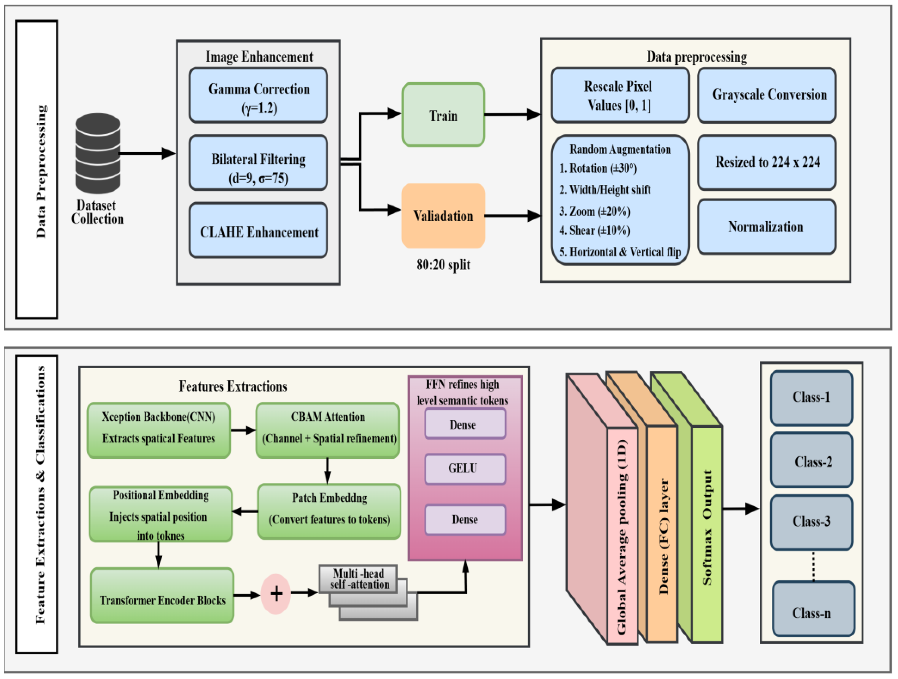
Figure 2.
Representative Sample Images from Each Class in the (a) CRC-VAL-HE-7k, (b) NCT-CRC-HE-100k, and (c) LC2500 Dataset.
Figure 2.
Representative Sample Images from Each Class in the (a) CRC-VAL-HE-7k, (b) NCT-CRC-HE-100k, and (c) LC2500 Dataset.
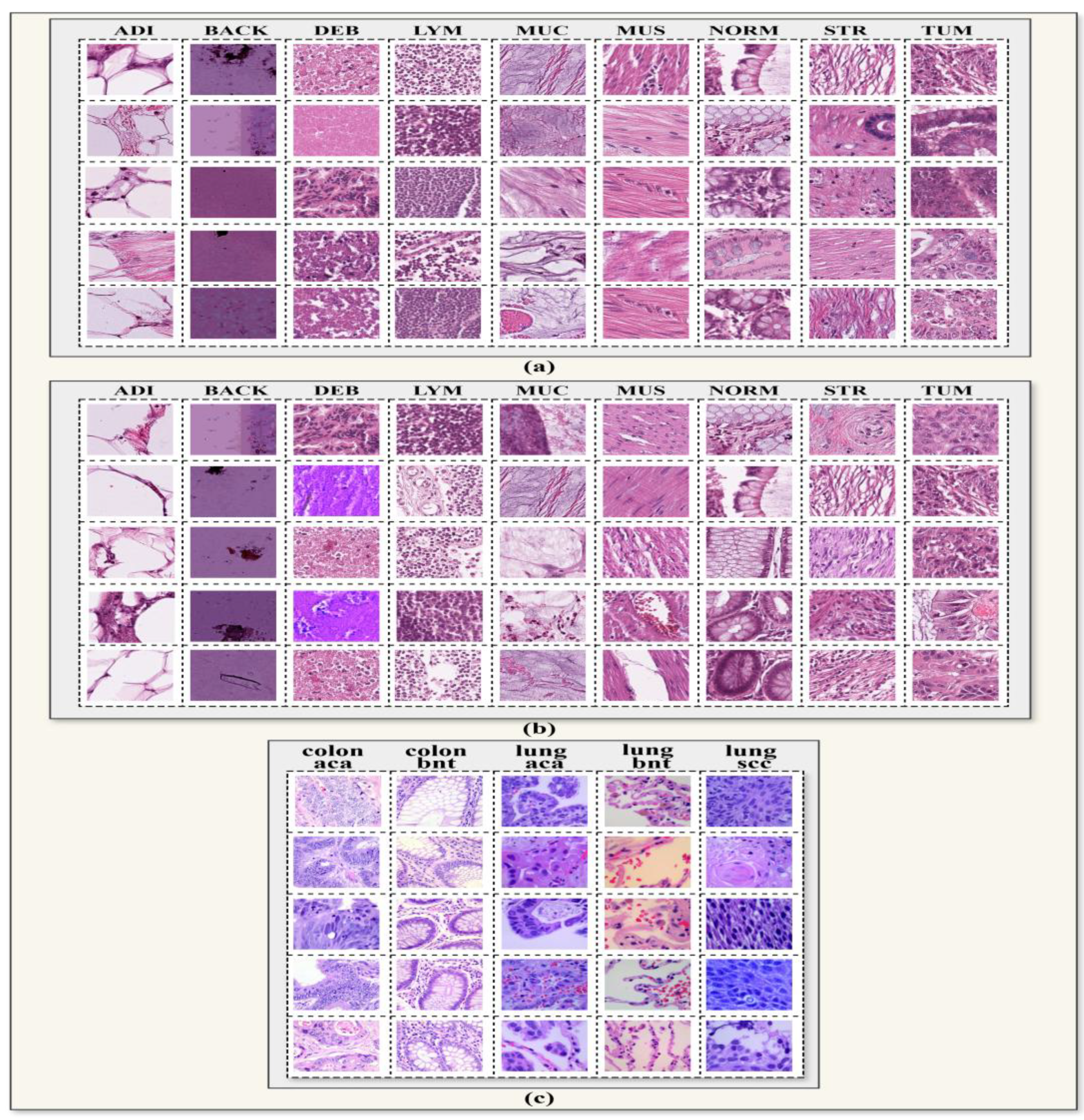
Figure 3.
Image enhancement process applied to histopathological samples, including gamma correction, bilateral filtering, and CLAHE to improve contrast and tissue structure visibility.
Figure 3.
Image enhancement process applied to histopathological samples, including gamma correction, bilateral filtering, and CLAHE to improve contrast and tissue structure visibility.
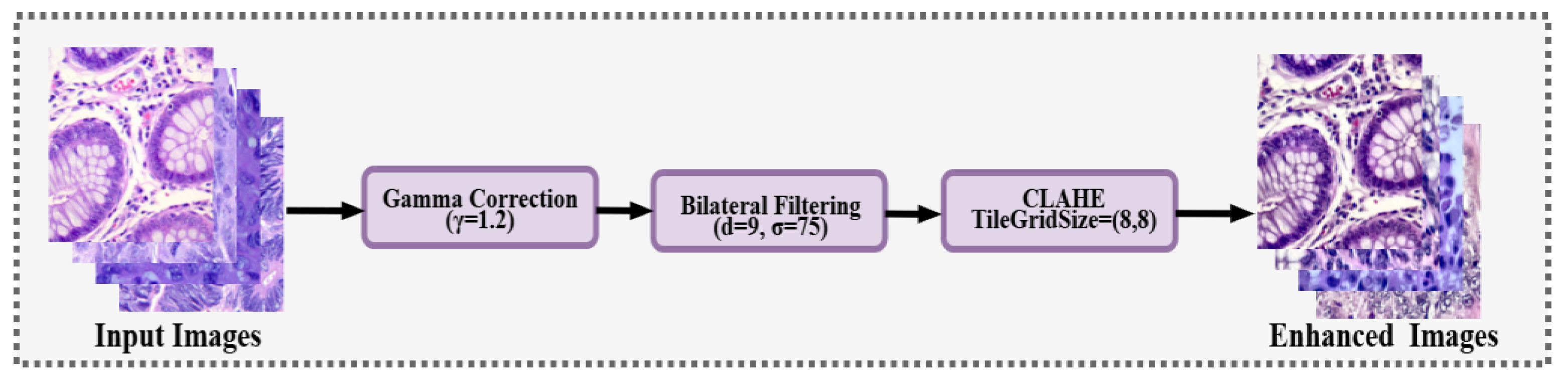
Figure 4.
Normal versus enhanced histopathological images from the (a) CRC-VAL-7K, (b) NCT-CRC-HE-100K, and (c) LC25000 datasets, demonstrating the visual improvements introduced by the enhancement pipeline.
Figure 4.
Normal versus enhanced histopathological images from the (a) CRC-VAL-7K, (b) NCT-CRC-HE-100K, and (c) LC25000 datasets, demonstrating the visual improvements introduced by the enhancement pipeline.
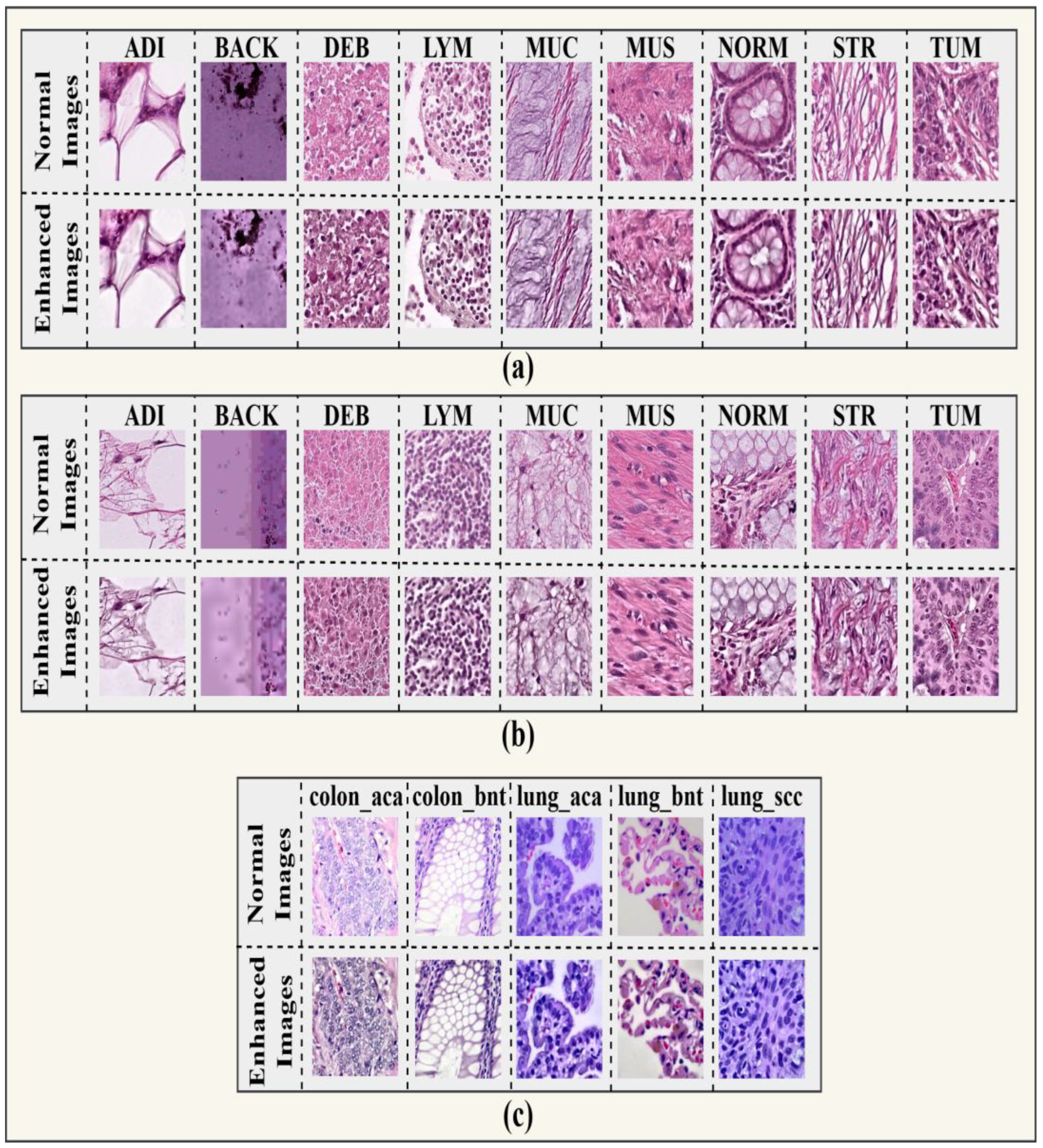
Figure 12.
The proposed model’s training and validation accuracy for NCT-CRC-100k.
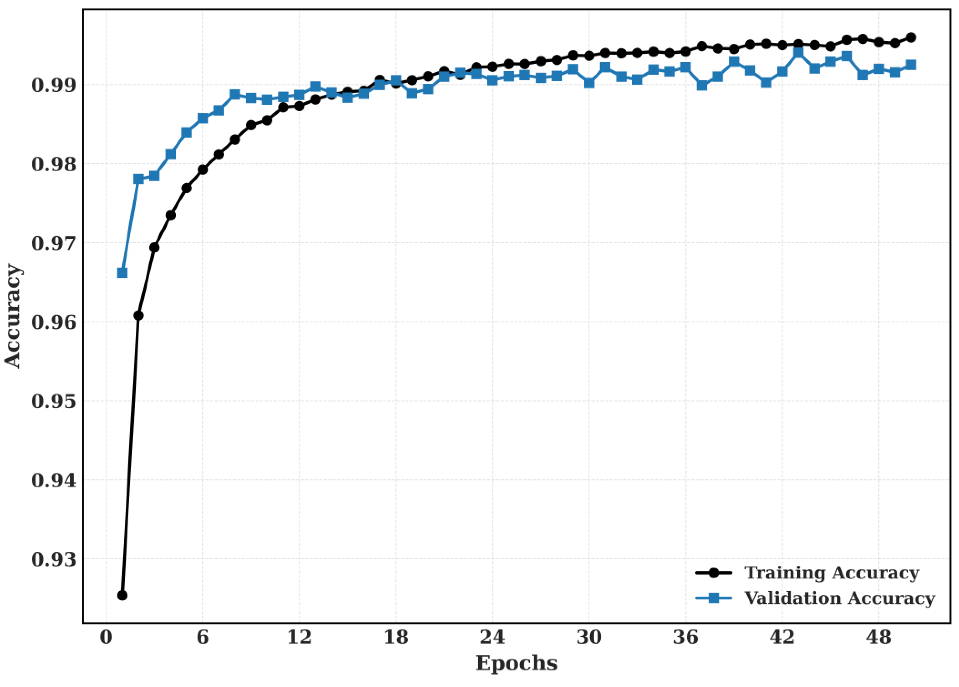
Figure 13.
The proposed model’s training and validation loss for NCT-CRC-HE-100k.
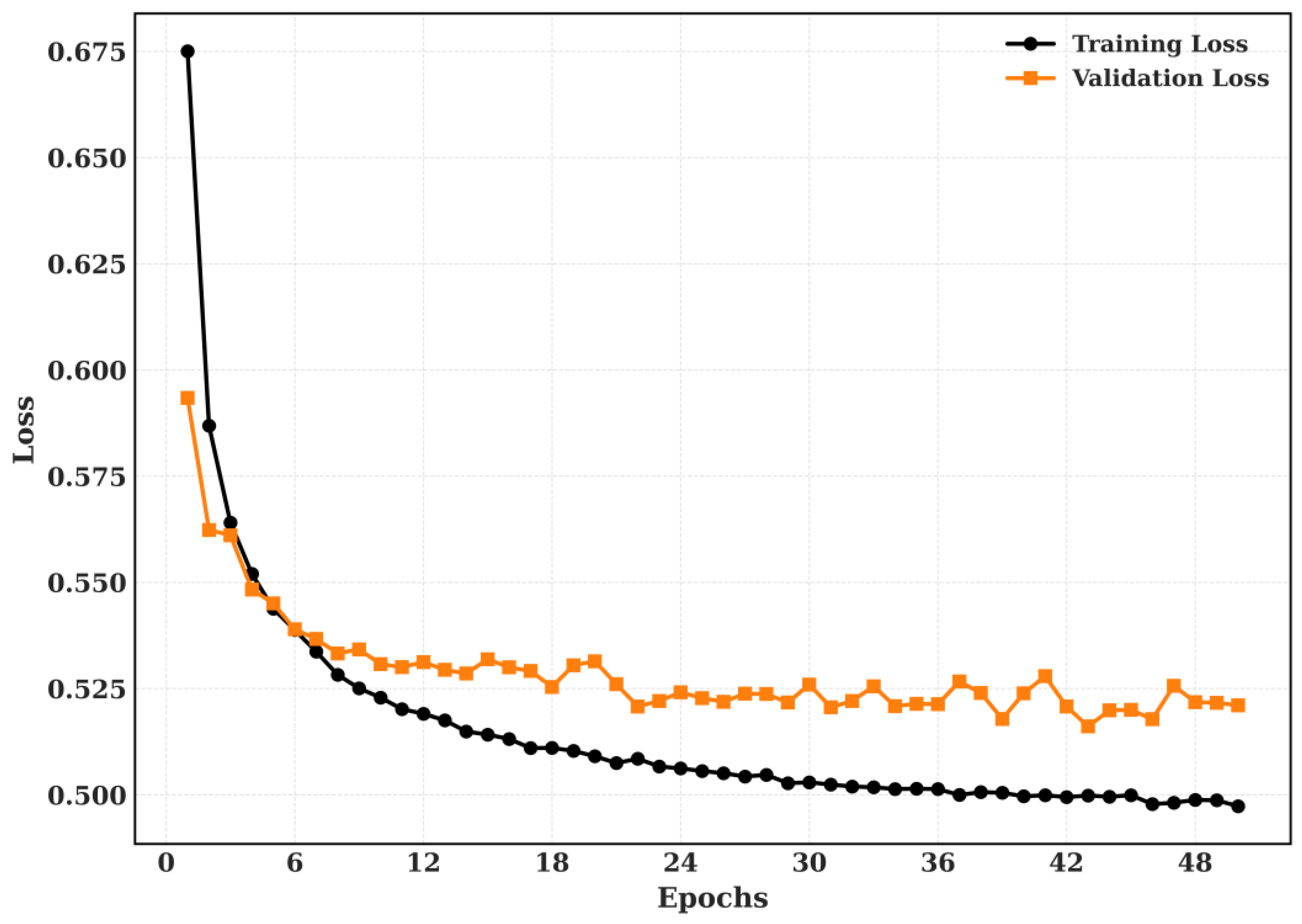
Figure 14.
The proposed model’s training and validation loss for LC-2500.
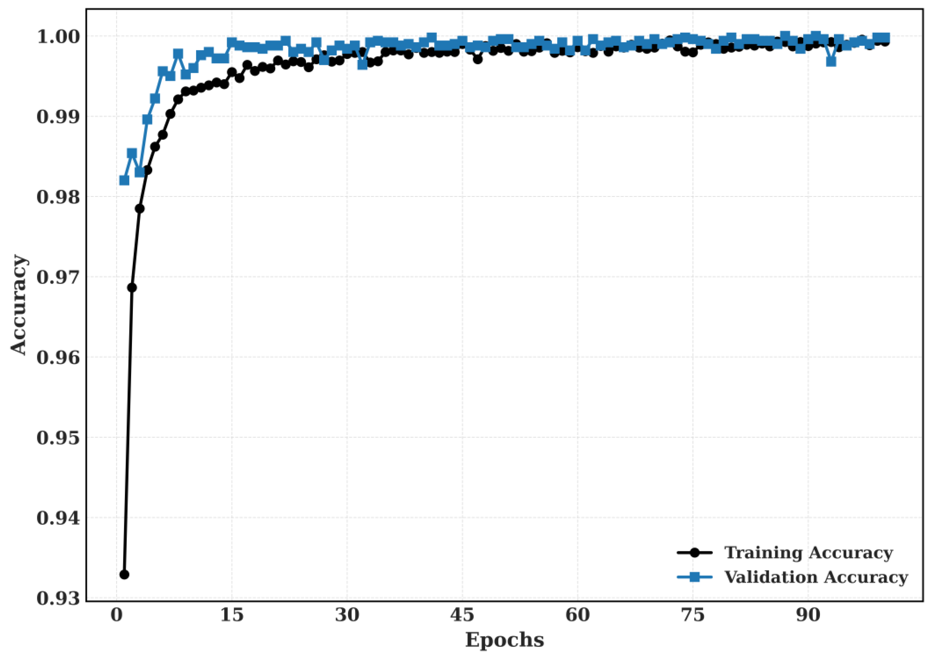
Figure 15.
The proposed model’s training and validation loss for LC-2500.
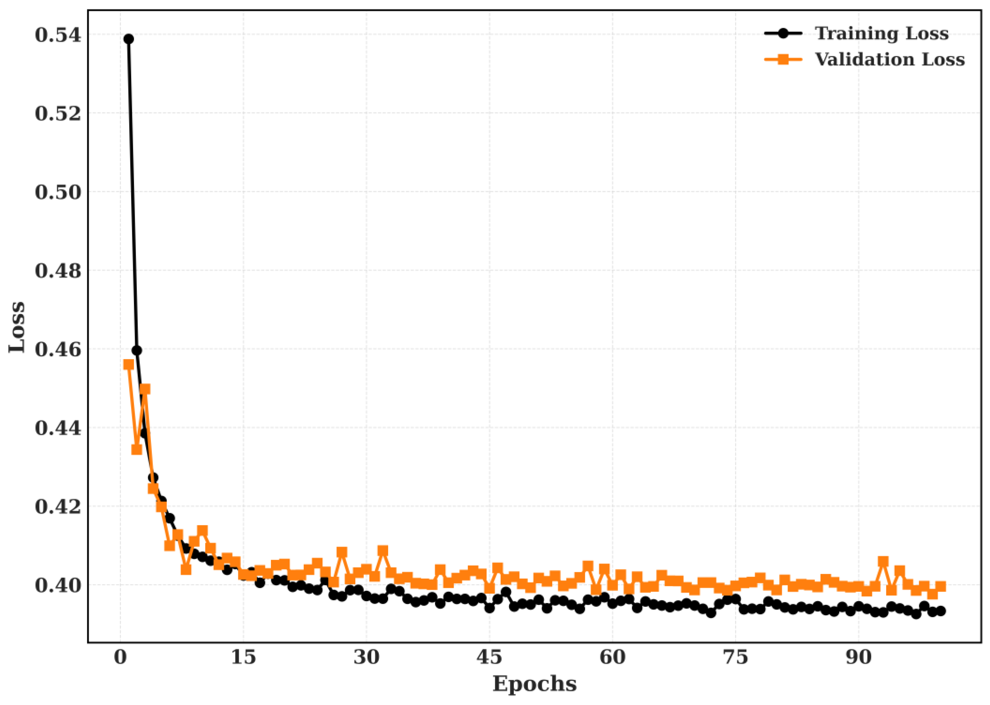
Figure 16.
t-SNE Visualization of Deep Feature Representations (CRC-VAL-HE-7k).
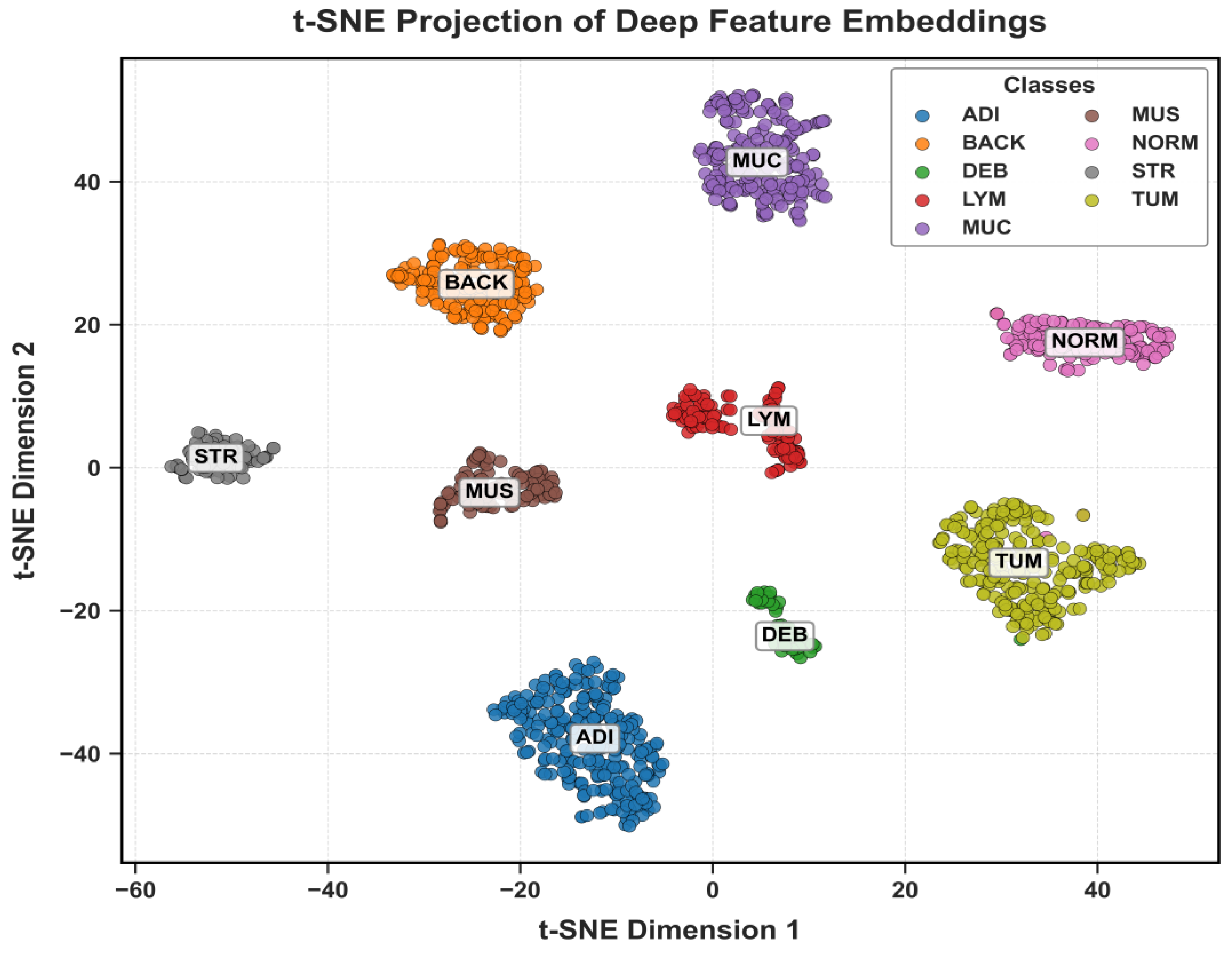
Figure 17.
t-SNE Visualization of Deep Feature Representations (NCT-CRC-HE-100k).
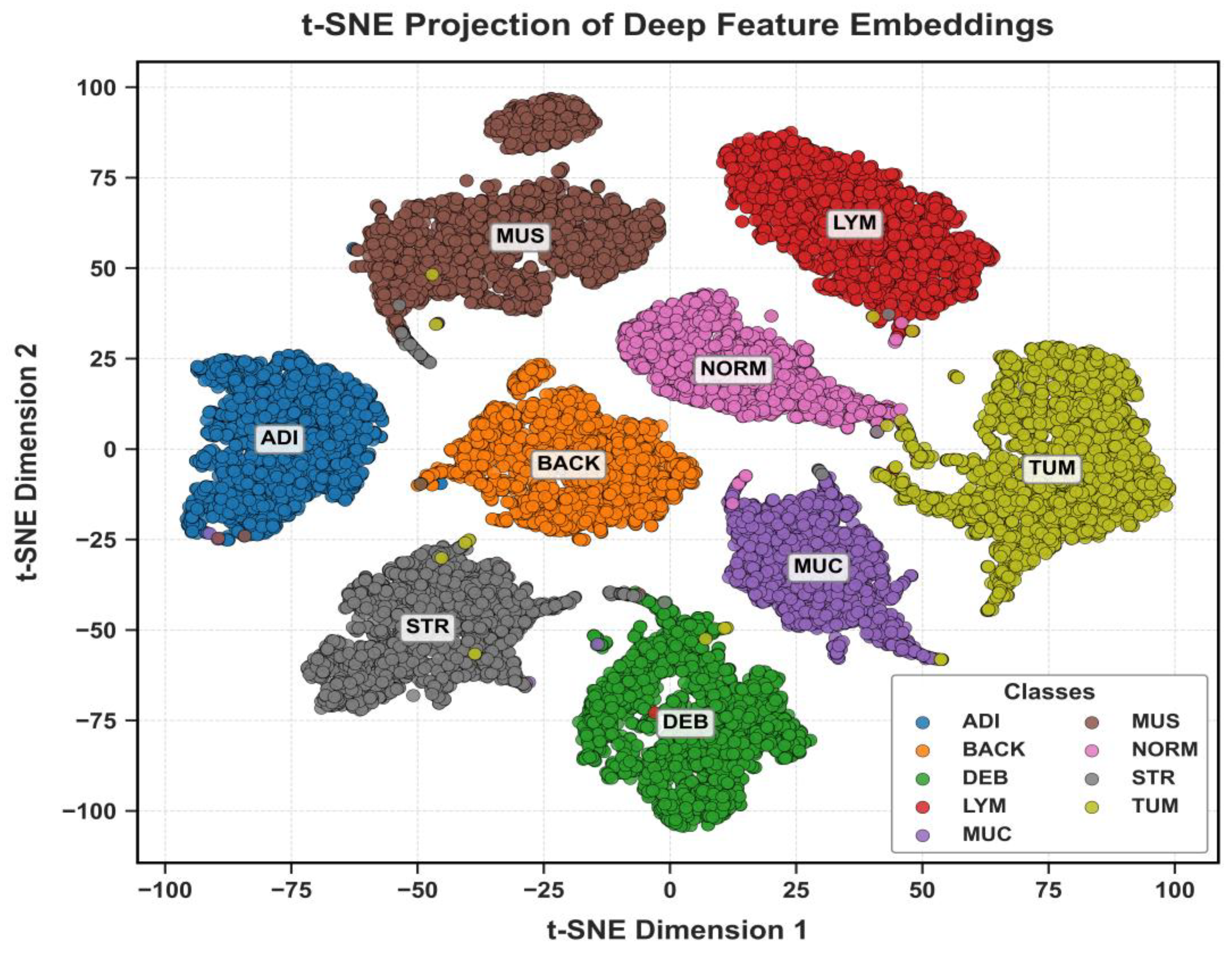
Figure 18.
t-SNE Visualization of Deep Feature Representations (LC-2500).
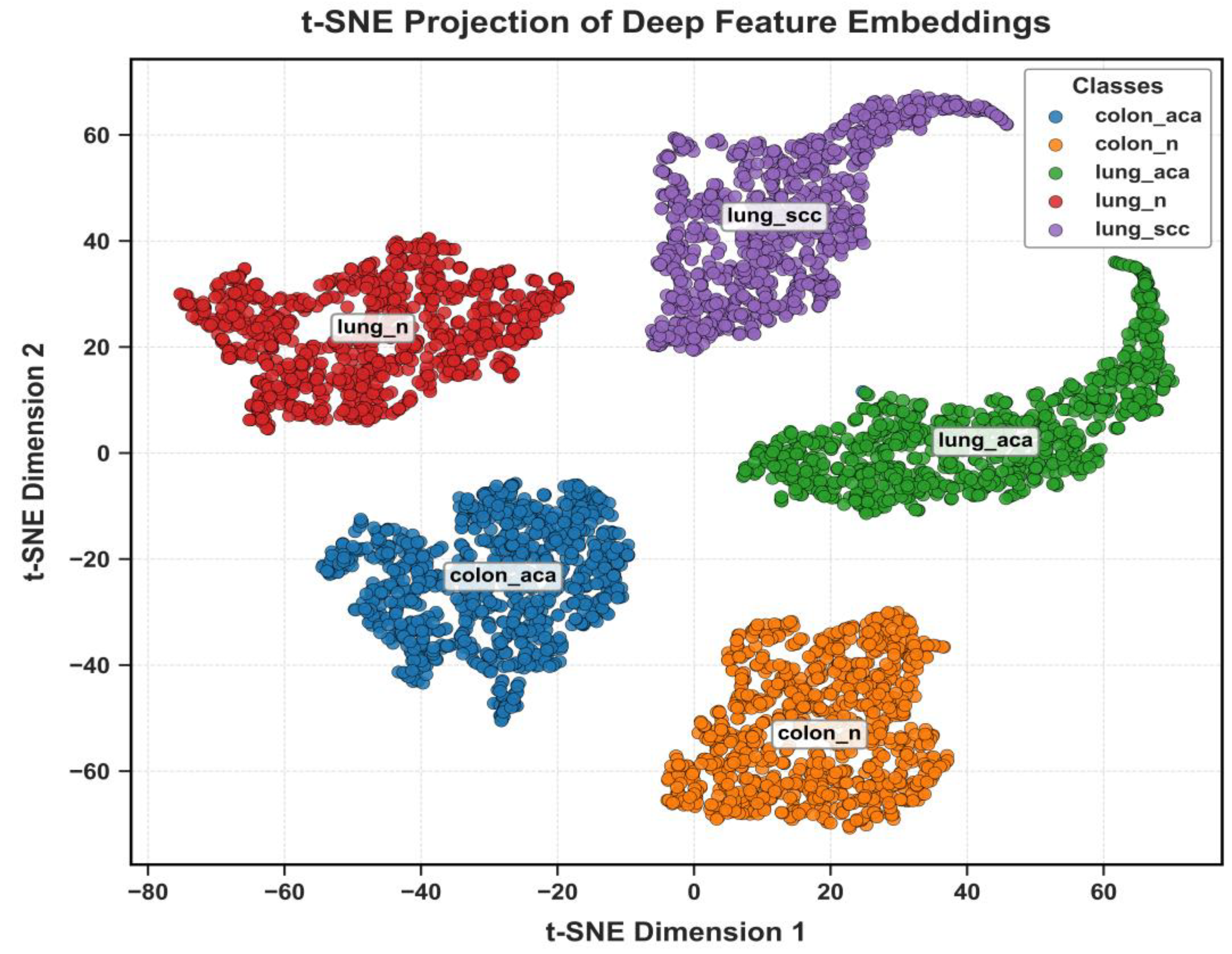
Figure 19.
ROC curve for the Proposed Model on (CRC-VAL-HE-7k).
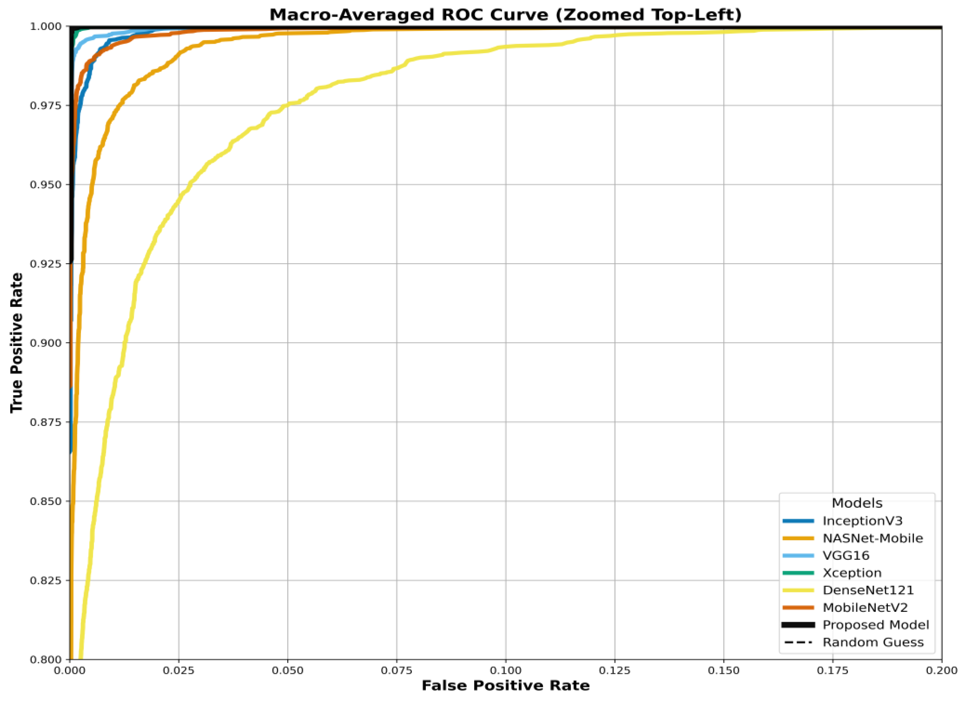
Figure 20.
ROC curve for the Proposed Model (NCT-CRC-100k).
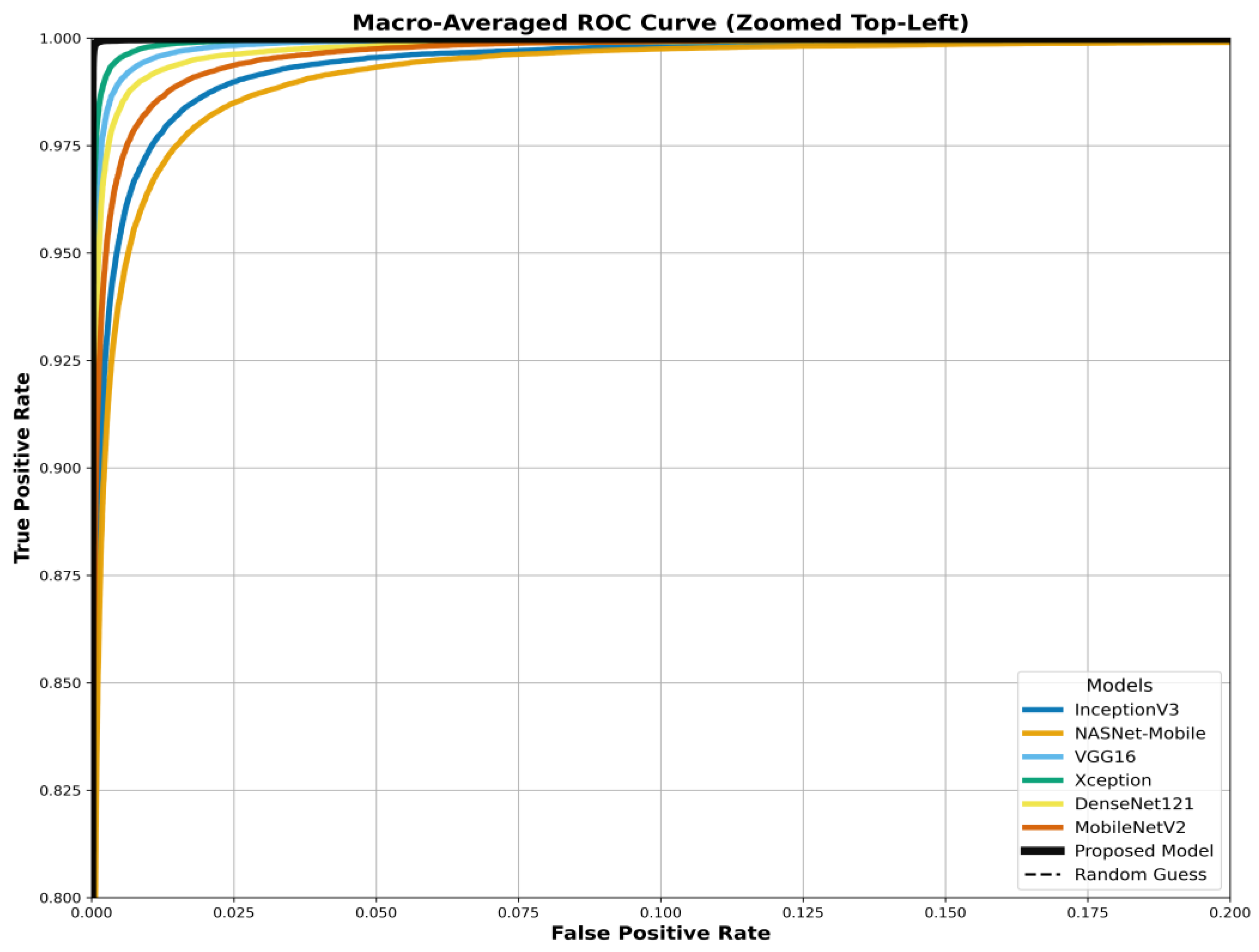
Figure 21.
ROC curve for the Proposed Model (LC-2500).
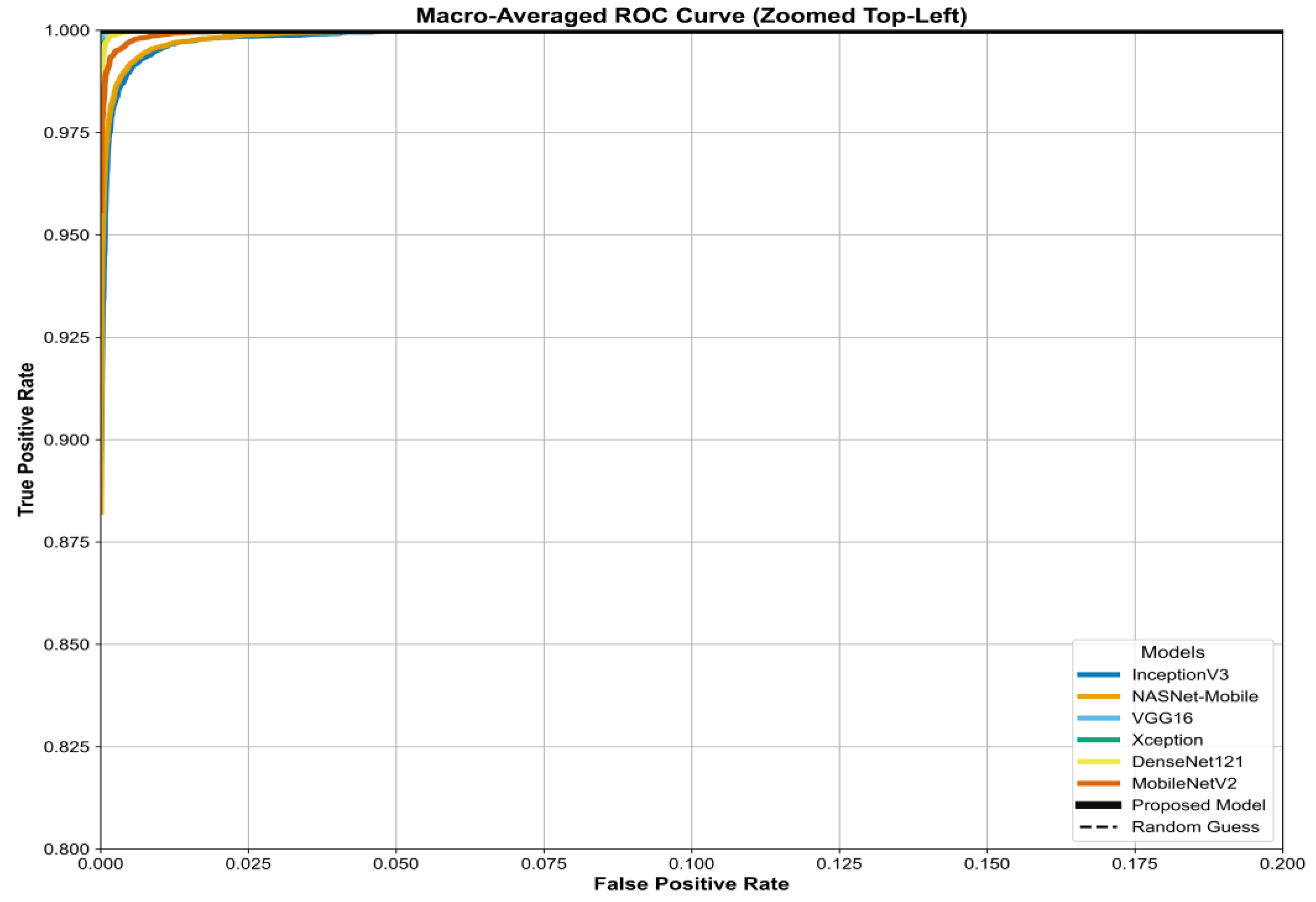
Figure 22.
The proposed model’s Layer wise feature extraction process on the input images. The Grad-CAM heatmaps highlight the model's focus on pathologically relevant regions.
Figure 22.
The proposed model’s Layer wise feature extraction process on the input images. The Grad-CAM heatmaps highlight the model's focus on pathologically relevant regions.
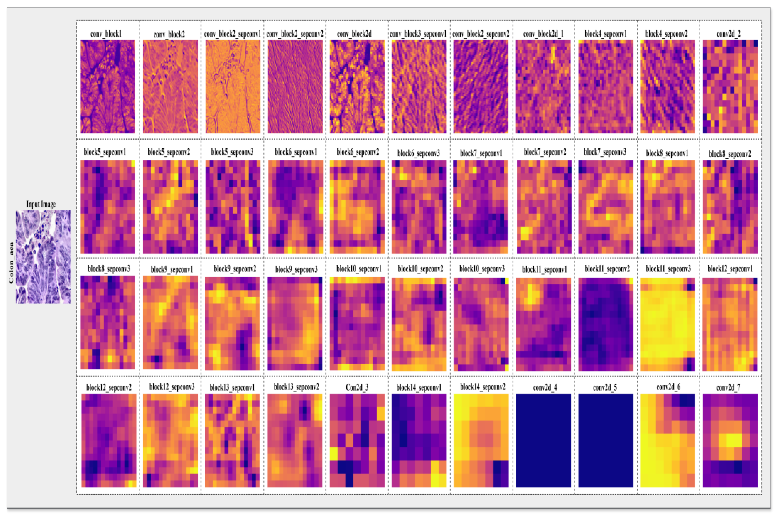
Figure 23.
The proposed model’s GradCAM visualization on CRC-VAL-HE-7k, NCT-CRC-HE-100k, and LC-2500 dataset.
Figure 23.
The proposed model’s GradCAM visualization on CRC-VAL-HE-7k, NCT-CRC-HE-100k, and LC-2500 dataset.
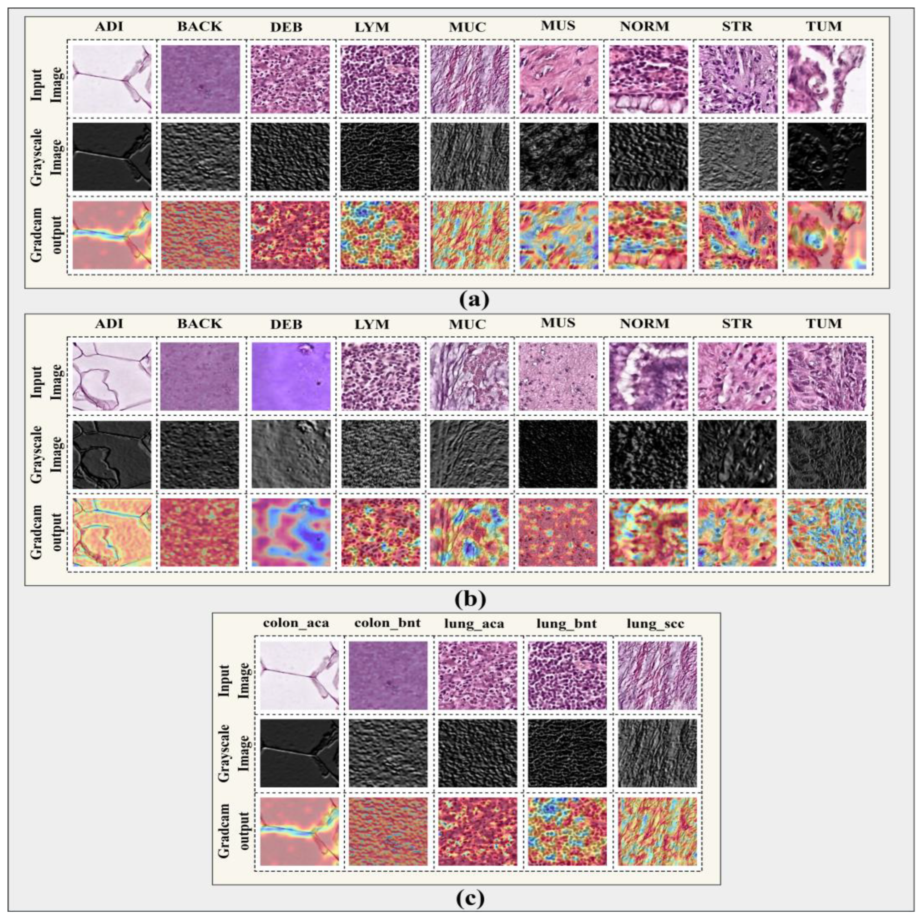
Table 2.
Class Distribution of the CRC-VAL-7k Dataset Following an 80–20% Train–Validation Split.
| Class | Total | Training (80%) | Validation (20%) |
|---|---|---|---|
| ADI | 1338 | 1070 | 268 |
| BACK | 847 | 678 | 169 |
| DEB | 339 | 271 | 68 |
| LYM | 634 | 507 | 127 |
| MUC | 1035 | 828 | 207 |
| MUS | 592 | 474 | 118 |
| NORM | 741 | 593 | 148 |
| STR | 421 | 337 | 84 |
| TUM | 1233 | 986 | 247 |
| Total | 7280 | 5744 | 1536 |
Table 3.
Class Distribution of the NCT-CRC-100k Dataset Following an 80–20% Train–Validation Split.
| Class | Total | Training (80%) | Validation (20%) |
|---|---|---|---|
| ADI | 15,020 | 12,016 | 3,004 |
| BACK | 10,566 | 8,453 | 2,113 |
| DEB | 11,512 | 9,210 | 2,302 |
| LYM | 11,557 | 9,246 | 2,311 |
| MUC | 8,896 | 7,117 | 1,770 |
| MUS | 13,536 | 10,829 | 2,707 |
| NORM | 8,763 | 7,010 | 1,753 |
| STR | 10,446 | 8,357 | 2,089 |
| TUM | 14,317 | 11,454 | 2,863 |
| Total | 104,113 | 83,192 | 20,921 |
Table 4.
Class Distribution of the LC25000 Dataset Following an 80–20% Train–Validation Split.
| Class | Total | Training (80%) | Validation (20%) |
|---|---|---|---|
| colon_aca | 5000 | 4000 | 1000 |
| colon_bnt | 5000 | 4000 | 1000 |
| lung_aca | 5000 | 4000 | 1000 |
| lung_scc | 5000 | 4000 | 1000 |
| lung_bnt | 5000 | 4000 | 1000 |
| Total | 25000 | 20000 | 5000 |
Disclaimer/Publisher’s Note: The statements, opinions and data contained in all publications are solely those of the individual author(s) and contributor(s) and not of MDPI and/or the editor(s). MDPI and/or the editor(s) disclaim responsibility for any injury to people or property resulting from any ideas, methods, instructions or products referred to in the content. |
© 2025 by the authors. Licensee MDPI, Basel, Switzerland. This article is an open access article distributed under the terms and conditions of the Creative Commons Attribution (CC BY) license (http://creativecommons.org/licenses/by/4.0/).
Copyright: This open access article is published under a Creative Commons CC BY 4.0 license, which permit the free download, distribution, and reuse, provided that the author and preprint are cited in any reuse.


