
Submitted:
15 December 2025
Posted:
16 December 2025
You are already at the latest version
Abstract
An infinite-horizon H∞ linear-quadratic control problem is considered. This problem has the following features: (i) the quadratic form of the control in the integrand of the cost functional is with a positive small multiplier (small parameter), meaning that the control cost is much smaller than the state cost; (ii) the current cost of the fast state variable in the cost functional is a positive semi-definite (but non-zero) quadratic form. These features require developing a significantly novel approach to asymptotic solution of the matrix Riccati algebraic equation associated with the considered H∞ problem by solvability conditions. Using this solution, an asymptotic analysis of the H∞ problem is carried out. This analysis yields parameter-free solvability conditions for this problem and a simplified controller solving this problem. An illustrative example is presented.
Keywords:
infinite-horizon H∞ control problem
; cheap control problem
; perturbed matrix Riccati algebraic equation
; asymptotic solution
; simplified controller
MSC: 93C05; 93C15; 93C73; 93D15; 93D20; 15A24; 65F45
1. Introduction
Uncertain dynamics systems are widely studied in the literature (see, e.g., [1,2,3,4,5,6,7,8,9,10,11,12,13,14] and references therein). The two most considered types of uncertainties are the following: (I) uncertainties which belong to a specified bounded set of an Euclidean space; (II) uncertainties which are quadratically integrable in a given interval (finite or infinite). For controlled systems with the second type of uncertainties (additive disturbances), the control problem is frequently considered (see, e.g., [1,3,4,5,8,13] and references therein).
In the present paper, we consider an infinite-horizon linear-quadratic control problem. The features of this problem are the following: (i) the current quadratic cost of the control in the cost functional is with a small multiplier ( is a small parameter), meaning that the control cost is much smaller than the state cost; (ii) the current quadratic cost of the fast state variable in the cost functional is a positive semi-definite (but non-zero) quadratic form. The first feature means that the considered problem is a cheap control problem.
Infinite-horizon cheap control problems and closed to these problems infinite-horizon zero-sum cheap control differential games have been studied in a number of works in the open literature. In these works, the following two types of the current quadratic cost of the fast state variable in the cost functional are considered: (a) the cost is a positive definite quadratic form (see, e.g., [13,15,16,17,18,19] and references therein); (b) the cost is zero (see, [16]). As it is aforementioned, in the present paper, we study an infinite-horizon cheap control problem in the case where the current quadratic cost of the fast state variable in the cost functional is a positive semi-definite (but non-zero) quadratic form. To the best of our knowledge, this case is completely novel.
The motivation of this purely theoretical paper is three-fold. The first motivation is to study asymptotically a considerably new class of cheap control problems. The second motivation is to carry out an asymptotic analysis of a new type of -dependent Riccati matrix algebraic equation associated with the original cheap control problem by solvability conditions. This analysis requires developing an essentially novel approach to the derivation of the asymptotic solution of the Riccati equation with respect to . The third motivation is to establish -free solvability conditions for the considered cheap control problem and to design a simplified controller, solving this problem.
The paper is organized as follows. In the next section, the problem is rigorously formulated. Objectives of the paper are stated. In Section 3-dependent solvability conditions for the formulated infinite-horizon cheap control problem are presented. Asymptotic solution of the -dependent Riccati matrix algebraic equation, appearing in these solvability conditions, is obtained in Section 4. Based on this asymptotic solution, -free conditions of solvability of the cheap control problem, valid for all sufficiently small , are established. In Section 5, the simplified controller, solving this cheap control problem for all sufficiently small , is designed. An academic illustrative example is presented in Section 6. Conclusions are placed in Section 7. Appendix A is devoted to the proof of the theorem justifying the validity of the simplified controller.
The following main notations are applied in the paper.
- denotes the n-dimensional real Euclidean space;
- denotes the Euclidean norm either of a vector () or of a matrix ();
- denotes the linear space of the functions square integrable in the interval ;
- denotes the norm in the space ;
- the superscript denotes the transposition either of a vector () or of a matrix ();
- denotes the identity matrix of dimension n;
- , where , ,..., , denotes the column block-vector of the dimension with the upper block , the next block and so on, and the lower block ;
- denotes the real part of a complex number .
2. Problem Formulation
Consider the system
where and , are the state vectors; is the control; is a disturbance; is an output; is a small parameter ; , and , , are given constant matrices of corresponding dimensions.
Assuming the fulfillment of the inclusions and , we consider the cost functional
where is a given constant called a performance level.
Let us consider the block vector
and let be a given number.
Definition 1.
The infinite horizon control problem with the dynamics (1)-(2) and the cost functional (6) is to design a controller such that, for any : (i) there exists the unique locally absolutely continuous solution , of the initial-value problem (1)-(2) with in the entire interval ; (ii) the following inequality is valid
Remark 1.
Due to the smallness of the parameter , the problem, formulated in Definition 1, is a cheap control problem, i.e., the problem where a control cost in the cost functional is much smaller than a state cost. In what follows, we call the problem with the dynamics (1)-(2) and the cost functional (6) the Cheap Control Problem (HCCP).
Remark 2.
Due to the equation (5), the matrices and are symmetric and at least positive semi-definite. In what follows, for the sake of timplicity (but without loss of the generality), we assume that the matrix has the form
Remark 3.
Using the non-singular control transformation , ( is a new control), we convert the HCCP into the equivalent control problem, which consists of the differential equations (1) and
and of the cost functional
The dynamic system of the new control problem is singularly perturbed. In this dynamic system is a slow state variable and is a fast state variable (see, e.g., [20]). Therefore, we call the state variables and of the HCCP a slow state variable and a fast state variable, respectively.
Objectives of this paper are:
- (I)
- to analyze asymptotically with respect to the HCCP using the method of its solution based on the game-theoretic matrix Riccati algebraic equation;
- (II)
- to derive an asymptotic solution to this Riccati equation;
- (III)
- to obtain -independent conditions for the existence of a controller solving the HCCP for all sufficiently small ;
- (IV)
- to design an asymptotically simplified controller solving the HCCP for all sufficiently small .
3. Solvability Conditions of the HCCP
First, we introduce the following block-form matrices:
where A and D are of the dimension ; B is of the dimension ; F is of the dimension .
Based on these matrices, let us construct the following matrix Riccati algebraic equation with respect to -matrix P:
where
We assume:
A1.
lie strictly inside the left-hand half-plane.
For a given , the equation (13) has a real solution such that:
- (a)
- ;
- (b)
- all roots , of the polynomial equation
Lemma 1.
Let the assumption A1 be valid. Then:
(i) is a positive semi-definite matrix;
(ii) the controller
solves the HCCP.
Proof.
We start with the item (i).
Consider the matrix
Since the matrices D and are symmetric and positive semi-definite, and the matrix is real and symmetric, then the matrix is symmetric and positive semi-definite.
Using the equation (17) and that is a solution of the equation (13), we obtain the following equality:
Let us consider this equality as a matrix Lyapunov algebraic equation (see, e.g., [21]) for with the matrix-valued coefficients and , and the matrix-valued non-homogeneity . Thus, using the item (b) of the assumption A1 and the results of [21], we can rewrite the equality (18) in the equivalent form
Since the matrices and are positive semi-definite, then the matrix in the right-hand side of the equality (19) is positive semi-definite. Hence, is positive semi-definite, which completes the proof of the item (i).
Proceed to the item (ii).
Consider the Lyapunov function
Let
where, for any given , is the solution of the initial-value problem (1)-(2) generated by the controller (see the equation (16)). Due to the assumption A1 and the form of , the aforementioned solution of the problem (1)-(2) exists, is unique and locally absolutely continuous in the entire interval .
Differentiating with respect to and using the assumption A1, we obtain the following expression:
Using the equations (1)-(2) with , as well as the equations (7),(12),(13),(14) and that is a solution of (13), we can convert (22) after a routine algebra to the following expression:
Finally, using the equation (16) and the notation
the expression (23) can be rewritten as:
where is the time realization of the controller along .
Let , () be any given vector and be any non-negative number. Let , be the solution of the system of the differential equations in (1)-(2), generated by the controller (see the equation (16)), the disturbance and the initial condition . Due to the item (b) of the assumption A1,
Let
The expression (27) implies the inequality
Remember that in this inequality is any -dimensional vector. This observation directly yields the validity of the item (i) of the lemma. Thus, the chain of the equations (20)-(30) represents an alternative proof of this item.
Based on the inequality (30), we continue to treat the expression (24). Since , this expression implies the following inequality for all :
Integrating this inequality from to any , using the equation (20) and taking into account that , we obtain
Since is a positive semi-definite matrix, the inequality (32) yields
which, along with the inclusion , implies
Since the matrix D is symmetric and positive semi-definite, the integral in the left-hand side of the inequality (34) is a non-decreasing function of and this function is bounded from above. Therefore, this integral has a finite limit for . This observation, along with the equations (6),(12) and the inequality (34), directly yields the inequality (8), where is given by the equation (16). Thus, the item (ii) of the lemma is proven. This completes the proof of the lemma □
Substituting into the system (1)-(2) and into the cost functional (6), and using the equations (7) and (12), we obtain after some rearrangement the following system and cost functional:
where
For the differential system (35), we consider the output equation
where is the unique symmetric positive semi-definite square root of the symmetrix positive semi-definite matrix .
Remark 4.
By virtue of Lemma 1 and the results of [3], the assumption A1 guarantees that the norm of the system (35),(38) satisfies the inequality
Moreover, for all and any number , the following inequality is valid:
Remark 5.
It should be noted the following. Lemma 1 is similar to the results of [13] (Theorem 3.4). However, this theorem is proven subject to the more restrictive assumptions than Lemma 1, while yields the stronger result than Lemma 1. Namely, in contrast to Lemma 1, Theorem 3.4 from [13] yields the positive definiteness of the solution to the matrix Riccati algebraic equation.
4. Asymptotic Solution of the Equation (13)
We derive the asymptotic solutions to the equation (13) (and, then, to the HCCP) subject to the condition
where , are the entries of the matrix (see the equation (9)).
4.1. Transformation of the Equation (13)
Due to the form of the matrix , the left-hand side of the equation (13) has the singularity for . In order to remove this singularity, we are going to transform this equation in a proper way. Namely, assuming the symmetry of the solution to (13) and using the form of the matrices and (see the equations (9),(41) and (14)), we look for this solution in the following block form:
where the matrices , and are of the dimensions , and , respectively, and these matrices are symmetric.
Let us partition the matrices A and into blocks as follows:
where
the blocks , , and , , are of the same dimensions as the corresponding blocks in (42); , .
In what follows, we derive the asymptotic solution of the equation (13) and, therefore, the asymptotic solution of the HCCP subject to the assumption:
A2..
In Section 4.3, the meaning of the assumption A2 is explained.
Using the equations (9),(12),(14),(41),(42),(43),(44) and the assumption A2, we can convert the equation (13) to the following equivalent form:
where
Remark 6.
The representation (42) and the system (46)-(51) differ considerably from the results of [13,22,23,24,25]. These representation and system are essentially novel results in the asymptotic analysis of parameter-dependent matrix Riccati algebraic equations with singularities, arising in infinite horizon control problems, differential games and optimal control problems.
4.2. Zero-Order Asymptotic Solution of the Set of the Equations (46)- (51)
We seek the zero-order solution of the set of the equations (46)- (51). The equations for this asymptotic solution are obtained by setting formally in (46)- (51) and replacing with , . Thus, we have
The equation (57) yields the unique symmetric positive definite solution
Substituting (60) into (55) and (58) and resolving the resulting equations with respect to and , respectively, we obtain
where .
Considering the equation (63) as an equation with respect to the unknown matrix , we can choose its solution as:
which, along with (62), yields
Now, using the equations (61),(64),(65), we can convert the equations (54) and (59) into the following equations for and , respectively:
In what follows, we assume:
A3. The equation (66) has a solution such that:
(a) ;
(b) all roots , of the polynomial equation
lie strictly inside the left-hand half-plane;
(c) all roots , of the polynomial equation
lie strictly inside the left-hand half-plane.
A4.
Remark 7.
4.3. Reduced Control Problem
Let us set in the Control Problem, consisting of the singularly perturbed system (1),(10) and the non-cheap control cost functional (11). Re-denoting the notations x, y, , w and in the resulting system and functional with , , , and , respectively, we obtain
It is seen that, in the set (72),(75), the variable , does not satisfy any equation. Hence, we can choose this variable to satisfy a desirable property of the system (72) and the functional (75). The latter means that can be chosen as a control in these system and functional. This observation means that the functional (75) depends on and , i.e., , where is the control, while is the disturbance. Similarly to Definition 1, we can formulate the control problem with the dynamics (72) and the cost functional (75).
Since the matrix is not invertible (see the equations (9),(41)), then the control problem (72),(75) cannot be solved by direct application of the method based on the matrix Riccati algebraic equation, i.e., it is singular (see, e.g., [13]). However, if the assumption A2 is fulfilled, the control problem (72),(75) becomes as:
where is the upper block of the control vector and it is the control in the problem (76)-(77). Since the matrix is positive definite, the problem (76)-(77) is regular, i.e., the method based on the matrix Riccati algebraic equation can be used for its solution. We call this control problem the Reduced Control Problem (RHCP). Thus, the assumption A2 guarantees the RHCP to be regular.
Consider the function
where is the solution of the problem (66) mentioned in the assumption A3 (items (a) and (c)).
Taking into account that , we obtain (similarly to Lemma 1) the following assertion.
Lemma 2.
Let the assumption A3 (items (a) and (c)) be valid. Then:
(i) is a positive semi-definite matrix;
(ii) the controller (78) solves the RHCP.
4.4. Justification of the Asymptotic Solution to the Equations (46)-(51)
Lemma 3.
Proof.
Let us transform the variables in the equations (46)- (51) as follows:
where , are new unknown matrices.
Consider the block-form matrix
Substitution of (80) into the equations (46)-(51) and use of the equations (54)-(59) and the block forms of the matrices , , A, (see the equations (14),(42), (43),(44)), yield after a routine matrix algebra the equation for
where
the matrix has the form
Taking into account the symmetry of the matrix , let us represent it in the block form
where the blocks have the same dimensions as the corresponding blocks of the matrix .
Substituting the expression for the matrix (see the equation (83)) into the equation (84) and using the equations (54)-(59),(64),(65), we obtain the estimates of the blocks in (85)
where is some sufficiently small number and is some number independent of .
Now, let us analyze the matrix . Taking into account the equations (60),(61),(64),(65), we can represent this matrix in the block form as:
where and denote matrices of corresponding dimensions satisfying the inequalities
is some number independent of .
Let us estimate the real parts of the eigenvalues of the matrix for all sufficiently small . For this purpose, first, we permute simultaneously the second and third block rows and columns of the matrix . This permutation yields the matrix
For any , the matrices and have the same set of eigenvalues.
Presenting the matrix as and applying the results of the work [28] (Theorem 2.1) in the particular (undelayed case) to the matrix , we can conclude the following. If the matrices and
are Hurwitz matrices, then there exists a positive number such that, for all , eigenvalues of the matrix satisfy the inequality
while the other eigenvalues satisfy the inequality
where and are some numbers independent of .
Proceed to the matrix . Using the equations (87),(90) and the inequalities (88), we obtain after a routine matrix algebra
Thus, is a Hurwitz matrix if and only if the matrices and are Hurwitz matrices. Due to the assumption A3 (item b), is a Hurwitz matrix. Due to Remark 7, is a Hurwitz matrix. Hence, is a Hurwitz matrix. Therefore, the inequalities (91) and (92) are satisfied.
Based on the inequalities (91),(92) and using the results of [21], we can rewrite the equation (82) in the equivalent form
where, for any given , the -matrix-valued function is the unique solution of the problem
We are going to estimate the matrix-valued function . For this purpose, let us partition it into blocks as:
where the blocks are of the same dimensions as the corresponding blocks in (42).
By virtue of the results of [28] (Theorem 2.3), we have the following estimates of these blocks:
where is some sufficiently small number; is some positive number independent of .
Now, let us apply the method of successive approximations to the equation (95). For this purpose, we consider the sequence of the matrices given as:
where ; ; the matrices have the block form
and the dimensions of the blocks in each of these matrices are the same as the dimensions of the corresponding blocks in (81).
Using the block form of the matrices , , , , (see the equations (14),(44),(85),(97),(100)), as well as using the estimates (86) and (98), we obtain the existence of a positive number such that, for any , the sequence converges in the linear space of -matrices. Moreover, the following inequalities are fulfilled:
where is some number independent of , r and l.
Thus, for any ,
is a solution of the equation (95) and, therefore, of the equation (82). Moreover, this solution has the block form similar to (81) and satisfies the inequalities
This observation, along with the equation (80), proves the lemma. □
Consider the matrix
where is the solution of the set of the equations (46)- (51) mentioned in Lemma 3.
Corollary 1.
Let the assumptions A2-A4 be valid. Then, there exists a positive number such that, for all , the assumption A1 is fulfilled with given by (101). Therefore, for these ε, all the statements of Lemma 1 are valid.
Proof.
First of all, let us note the following. Since the set of the equations (46)- (51) is equivalent to the equation (13) and is a solution of (46)- (51) for all , then the matrix is a solution of (13). Since the matrix is symmetric, then the item (a) of the assumption A1 is fulfilled for all .
Proceed to the proof of the fulfillment of the item (b).
Consider the matrix given in the equation (37).
Using the block form of the matrices , A and (see the equations (14),(43) and (101)), as well as Lemma 3, the assumption A2 and the equations (60),(61),(64),(65), we can represent the matrix in the following block form
where denotes a matrix of corresponding dimension satisfying the inequality
are some numbers independent of .
Let us estimate the real parts of the eigenvalues of the matrix for all sufficiently small . This estimation is done quite similarly to such an estimation for the matrix in the proof of Lemma 3. Namely, first, we permute simultaneously the second and third block rows and columns of the matrix which yields the matrix
For any , the matrices and have the same set of eigenvalues.
Presenting the matrix as and applying the results of the work [28] (Theorem 2.1) in the particular (undelayed case) to the matrix , we can conclude the following. If the matrices and
are Hurwitz matrices, then there exists a positive number such that, for all , eigenvalues of the matrix satisfy the inequality
while the other eigenvalues satisfy the inequality
where and are some numbers independent of .
Proceed to the matrix . Using the equations (102),(105) and the inequalities (88),(103), we obtain after a routine matrix algebra
Thus, is a Hurwitz matrix if and only if the matrices and are Hurwitz matrices. Due to the assumption A3 (item c), is a Hurwitz matrix. Due to Remark 7, is a Hurwitz matrix. Hence, is a Hurwitz matrix. Therefore, the inequalities (106) and (107) are satisfied, meaning that the item (b) of the assumption A1 is fulfilled for all . Since both items of the assumption A1 are fulfilled for all , then the statements of Lemma 1 are valid for these . Thus, the corollary is proven. □
Remark 9.
Corollary 1 presents the ε-free solvability conditions of the HCCP.
5. Simplified Controller for the HCCP
Consider the following controller for the HCCP:
where the matrix B is given in (12) and the matrix is given in (83).
Comparing the equations (16) and (110) with each other, one can conclude that the controller is obtained from the controller by replacing in the latter with .
Substituting into the system (1)-(2) and into the cost functional (6), and using the equations (7),(12) and (14), we obtain after some rearrangement the following system and cost functional:
where
Remark 10.
Theorem 1.
Let the assumptions A2-A4 be valid. Then, there exists a positive number such that, for all , the controller solves the HCCP.
Proof of the theorem is presented in Appendix A.
For the differential system (111), we consider the output equation
where is the unique symmetric positive semi-definite square root of the symmetrix positive semi-definite matrix .
Similarly to Remark 4, we have the following remark.
6. Illustrative Example
Consider a particular case of the HCCP with the following data:
yielding
Let be the solution of the matrix Riccati algebraic equation (13) for the matrix-valued coefficients given in (119).
In this example, was calculated numerically using the MATLAB function [style=Matlab-editor]icare(A,[],D,[],[],[],-(Su-Sw)). Numerical simulation shows that the equation (13) with the data (119) admits the unique symmetric stabilizing solution for .
In Figure 1 and Figure 2, the real parts of the eigenvalues , of the closed-loop matrix (see the equation (37)) are depicted for .
It is seen that , for all , i.e., the MATLAB function [style=Matlab-editor]icare returns the symmetric stabilizing solution of (13),(119) meaning that the assumption A1 is satisfied for all .
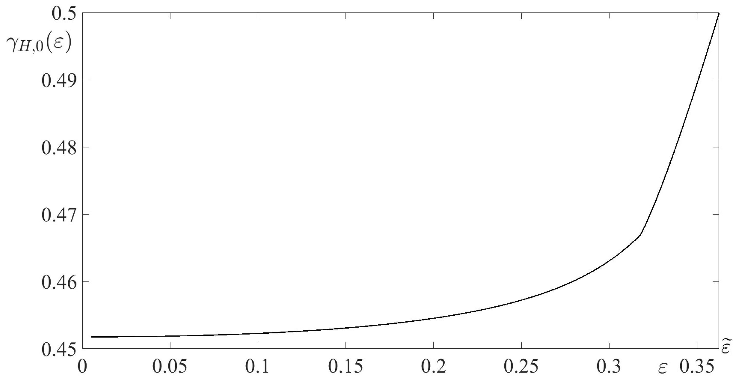
Figure 3 presents the norm of the system (35),(38) in this example as a function of . It is seen that for all , which illustrates Remark 4. The norm was calculated by implementing the MATLAB code
[style=Matlab-editor]Acl=A-Su*P;
[style=Matlab-editor]Dcl=D+P*Su*P;
[style=Matlab-editor]Ccl=sqrtm(Dcl);
[style=Matlab-editor]system=ss(Acl,F,Ccl,0);
[style=Matlab-editor]hinfn=hinfnorm(system);
One can observe that, in agreement with the results of [3],
Using the equations (12),(14),(43)-(45),(118), we obtain that in this example the system (46)-(51) becomes as:
where , , , , and are scalar unknowns.
Using the results of the Section 4.2 and the data (118) of the example, we obtain the following components of the solution to the system (122):
The components and satisfy the equations
and
respectively.
The component satisfies the equation
Let us start with the equation (124). This quadratic equation has two solutions and . It is directly verified that satisfies the assumption A3, while does not satisfy this assumption. Thus,
which, along with (126), yields
Proceed to the equation (125). Before solving this equation, let us check the fulfillment of the assumption A4.
Due to the data (118) of the example, , and . Substituting these values into the equation (70), we immediately obtain the fulfillment of the assumption A4. Therefore, the equation (125) has the solution mentioned in Remark 7. This solution is
The absolute values of the errors , defined in (80), for , and for are shown in Figure 4 and Figure 5, respectively. For the sake of clear demonstration, the errors are depicted for . It is seen that these errors are of the order , which illustrates Lemma 3.
Furthermore, using the equations (7),(110),(118),(130), we obtain the simplified controller in this example
where ; x, , are scalar state variables; x is a slow state variable, while is a fast state variable.
Moreover, in this example the matrix-valued coefficient of the closed-loop system (111) is
and (111) becomes
where .
The matrix , appearing in the cost functional (112), becomes
By a routine algebra, it is shown that the eigenvalues of the matrix (132) are
and these eigenvalues satisfy the inequalities for all . Thus, the simplified controller (131) stabilizes the system (1)-(2) with the data (118) for all .
In this example, the Riccati algebraic equation (A1) was solved numerically using the MATLAB function [style=Matlab-editor]icare. Numerical simulation showed that this equation admits the unique symmetric stabilizing solution for .
Thus, the simplified controller (131) solves the HCCP for .
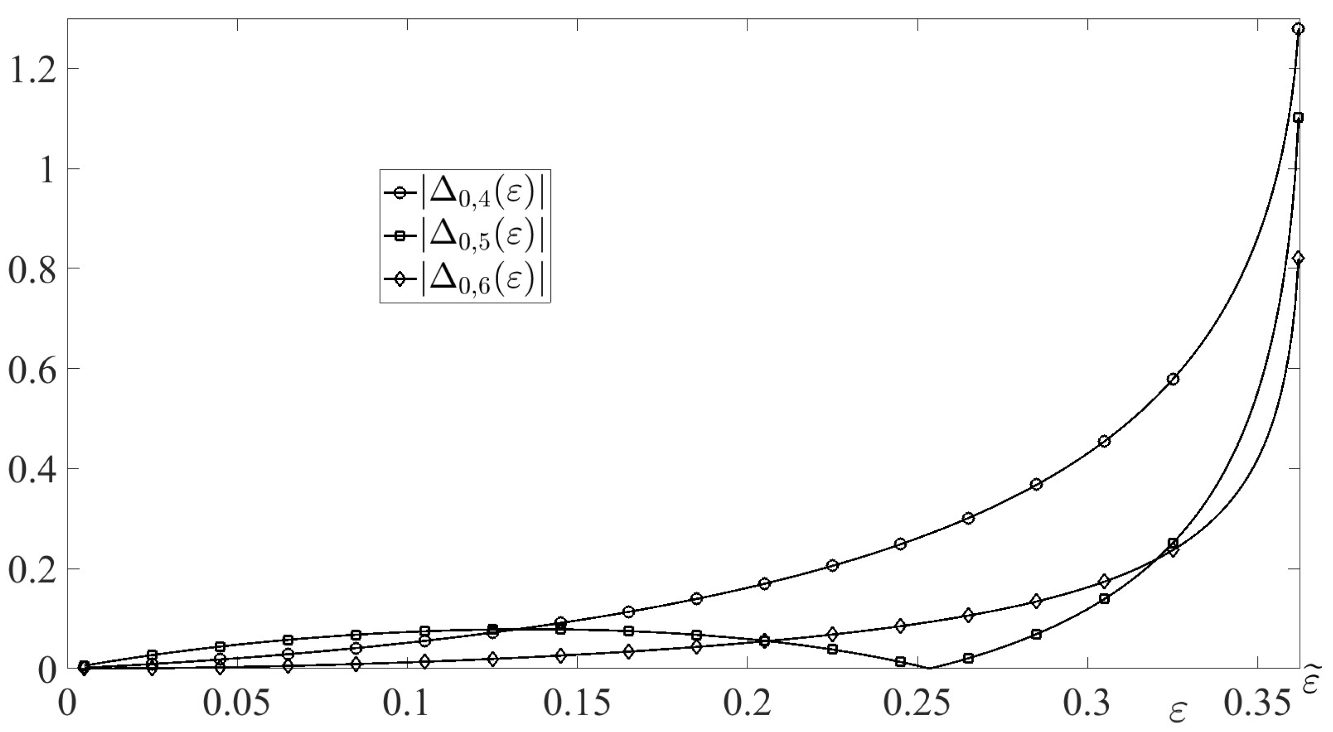
The absolute values of the errors for , and for are shown in Figure 6 and Figure 7, respectively, for . It is seen that these errors are of the order , which illustrates Lemma A2.
In Figure 8, the norm of the differential system (133) with the output (115) and the matrix , given by (134), is depicted for . It is seen that, for these values of , . The latter means that the simplified controller (131) solves the HCCP (1)-(2),(6) with the data (118) not only for all and , but also for all and any performance level instead of in the cost functional.
In addition, let us note that, similarly to (120), .
7. Conclusions
In this paper, an infinite-horizon control problem for a linear differential equation and a quadratic cost functional was studied in the case where the control cost is much smaller than the state cost. This smallness is due to the presence of the small multiplier ( is a small parameter) in the control cost. Because of this feature, the considered problem is a cheap control problem. One more feature of this problem is the following. The problem’s dynamics has both, slow and fast, state variables, and the current quadratic cost of the fast state variable in the cost functional is a positive semi-definite (but non-zero) quadratic form. By the solvability conditions, the solution of the considered control problem was reduced to the solution of the game-theoretic matrix Riccati algebraic equation perturbed by the small parameter . This equation represents a new type of -dependent matrix Riccati algebraic equations arizing in the control theory. The zero-order asymptotic solution to the aforementioned matrix Riccati algebraic equation was derived. This derivation requires the developing the considerably novel approach. Based on the asymptotic solution to the matrix Riccati algebraic equation, the -free conditions, providing the existence of the solution to the considered cheap control problem for all sufficiently small , were established. The simplified controller, solving this problem for all sufficiently small , was designed. Using the theoretical results, the academic example was solved. Numerical simulation in this example shows that a very accurate approximation of the solution to the cheap control problem is obtained even for not too small values of .
Appendix A. Proof of Theorem 1
Proof of Theorem 1 is based on two auxiliary lemmas.
Appendix A.1. Auxiliary Lemmas
Lemma A1.
Let the assumptions A2-A4 be valid. Then, there exists a positive number such that, for all , the real parts of all eigenvalues of the matrix are smaller than some negative number independent of ε.
Proof.
The lemma is proven just similarly to the proof of Corollary 1 (the property of the matrix ). □
Consider the following matrix Riccati algebraic equation with respect to the -matrix :
Lemma A2.
Let the assumptions A2-A4 be valid. Then, there exists a positive number such that, for all , the equation (A1) has a solution of the block form
where the matrices , and are of the dimensions , and , respectively, and these matrices are symmetric.
Moreover, the matrices , satisfy the inequalities
where the matrices , are obtained in Section 4.2; is some constant independent of ε.
Proof.
The lemma is proven quite similarly to Lemma 3. □
Appendix A.2. Main Part of the Proof
Consider the Lyapunov-like function
where is the solution of the equation (A1), mentioned in Lemma A2; .
Let
where, for any given , is the unique solution of the initial-value problem (111). This solution is locally absolutely continuous in the entire interval .
Differentiating with respect to , we obtain the following expression:
Using the equations (111),(A1), we can convert (A4) after a routine algebra to the following expression:
Let be any given vector and be any non-negative number. Let , be the solution of the differential equation in (111), generated by the disturbance and the initial condition . Due to Lemma A1,
Let
Since is a positive semi-definite matrix for all , the expression (A9) yields the inequality
In this inequality is any -dimensional vector. This observation directly yields the positive semi-definiteness of the matrix for all .
Since , this expression implies the inequality
Integrating this inequality from to any , using the equation (A2) and taking into account that , we obtain
Since is a positive semi-definite matrix, the inequality (A12) yields
which, along with the inclusion , implies
Since the matrix is symmetric and positive semi-definite for all , the integral in the left-hand side of the inequality (A14) is a non-decreasing function of and this function is bounded from above. Therefore, this integral has a finite limit for . This observation, along with the equation (112) and the inequality (A13), directly yields the inequality (114). This conclusion, along with Remark 10, completes the proof of the theorem.
References
- Doyle, J.C.; Glover, K.; Khargonekar, P.P.; Francis, B. State-space solution to standard H2 and H∞ control problem. IEEE Trans. Autom. Control 1989, 34, 831-–847. [Google Scholar] [CrossRef]
- Doyle, J.; Francis, B.; Tannenbaum, A. Feedback Control Theory; Macmillan Publishing Co.: London, UK, 1990. [Google Scholar]
- Baar, T.; Bernhard, P. H∞-Optimal Control and Related Minimax Design Problems: A Dynamic Games Approach; Birkhauser: Boston, MA, USA, 1991. [Google Scholar]
- Petersen, I.; Ugrinovski, V.; Savkin, A.V. Robust Control Design Using H∞ Methods; Springer: London, UK, 2000. [Google Scholar]
- Gershon, E.; Shaked, U.; Yaesh, I. H∞-Control and Estimation of State-multiplicative Linear Systems. In Lecture Notes in Control and Information Science Series; Springer: London, UK, 2005; Volume 318. [Google Scholar]
- Martynyuk, A.A.; Martynyuk-Chernienko, Yu.A. Uncertain Dynamical Systems: Stability and Motion Control; CRC Press: Florida, USA, 2011. [Google Scholar]
- Glizer, V.Y.; Turetsky, V. Robust Controllability of Linear Systems; Nova Science Publishers: New-York, NY, USA, 2012. [Google Scholar]
- Chang, X.H. Robust Output Feedback H∞ Control and Filtering for Uncertain Linear Systems; Springer: Berlin, Germany, 2014. [Google Scholar]
- Fridman, L.; Poznyak, A.; Rodrguez, F.J.B. Robust Output LQ Optimal Control via Integral Sliding Modes; Birkhuser: Basel, Switzerland, 2014. [Google Scholar]
- Petersen, I.R.; Tempo, R. Robust control of uncertain systems: classical results and recent developments. Autom. J. IFAC 2014, 50, 1315–-1335. [Google Scholar] [CrossRef]
- Yedavalli, R.K. Robust Control of Uncertain Dynamic Systems: A Linear State Space Approach; Springer: New York, NY, USA, 2014. [Google Scholar]
- Kersten, J.; Rauh, A.; Aschemann, H. Analyzing uncertain dynamical systems after state-space transformations into cooperative form: verification of control and fault diagnosis. Axioms 2021, 10, 88. [Google Scholar] [CrossRef]
- Glizer, V.Y.; Kelis, O. Singular Linear-Quadratic Zero-Sum Differential Games and H∞ Control Problems: Regularization Approach; Birkhauser: Basel, Switzerland, 2022. [Google Scholar]
- Aggarwal, V.; Agarwal, M. Control of uncertain systems. In Springer Handbook of Automation; Nof, S.Y., Ed.; Springer Handbooks, Springer: Cham, 2023. [Google Scholar]
- Petersen, I.R. Linear-quadratic differential games with cheap control. Syst. Control Lett. 1986, 8, 181–-188. [Google Scholar]
- Toussaint, G.J.; Baar, T. Achieving nonvanishing stability regions with high-gain cheap control using H∞ techniques: the second-order case. Systems Control Lett. 2001, 44, 79–89. [Google Scholar] [CrossRef]
- Glizer, V.Y. H∞ cheap control for a class of linear systems with state delays. J. Nonlinear Convex Anal. 2009, 10, 235–259. [Google Scholar]
- Glizer, V.Y. Solution of a singular H∞ control problem for linear systems with state delays. In Proceedings of the 2013 European Control Conference published on-line at IEEE Xplore Digital Library, 2013; pp. 2843–2848. Available online: http://ieeexplore.ieee.org/.
- Glizer, V.Y.; Kelis, O. Singular infinite horizon zero-sum linear-quadratic differential game: saddle-point equilibrium sequence. Numer. Algebra Control Optim. 2017, 7, 1–20. [Google Scholar] [CrossRef]
- Vasil’eva, A.B.; Butuzov, V.F.; Kalachev, L.V. The Boundary Function Method for Singular Perturbation Problems; SIAM Books: Philadelphia, PA, USA, 1995. [Google Scholar]
- Gajic, Z.; Qureshi, M.T.J. Lyapunov Matrix Equation in System Stability and Control; Dover Publications: Mineola, NY, USA, 2008. [Google Scholar]
- Pan, Z.; Baar, T. H∞-optimal control for singularly perturbed systems. Part I: Perfect state measurements. Autom. J. IFAC 1993, 29, 401–423. [Google Scholar] [CrossRef]
- Pan, Z.; Baar, T. H∞-optimal control for singularly perturbed systems. Part II: Imperfect state measurements. IEEE Trans. Autom. Control 1994, 39, 280–299. [Google Scholar]
- Gajic, Z.; Lim, M.T. Optimal Control of Singularly Perturbed Linear Systems and Applications. In High Accuracy Techniques; Marsel Dekker: New York. NY, 2001. [Google Scholar]
- O’Reilly, J. Partial cheap control of the time-invariant regulator. Internat. J. Control 1983, 37, 909–927. [Google Scholar] [CrossRef]
- Kalman, R.E. Contributions to the theory of optimal control. Bol. Soc. Mat Mexicana 1960, 5, 102–-119. [Google Scholar]
- Daletskii, Ju.L.; Krein, M.G. Stability of Solutions Of Differential Equations In Banach Space. In Translations of Mathematical Monographs; American Mathematical Society: Providence, RI, USA, 1974; Volume 43. [Google Scholar]
- Glizer, V.Y. Blockwise estimate of the fundamental matrix of linear singularly perturbed differential systems with small delay and its application to uniform asymptotic solution. J. Math. Anal. Appl. 2003, 278, 409–-433. [Google Scholar] [CrossRef]
Figure 1.
Real parts of and .
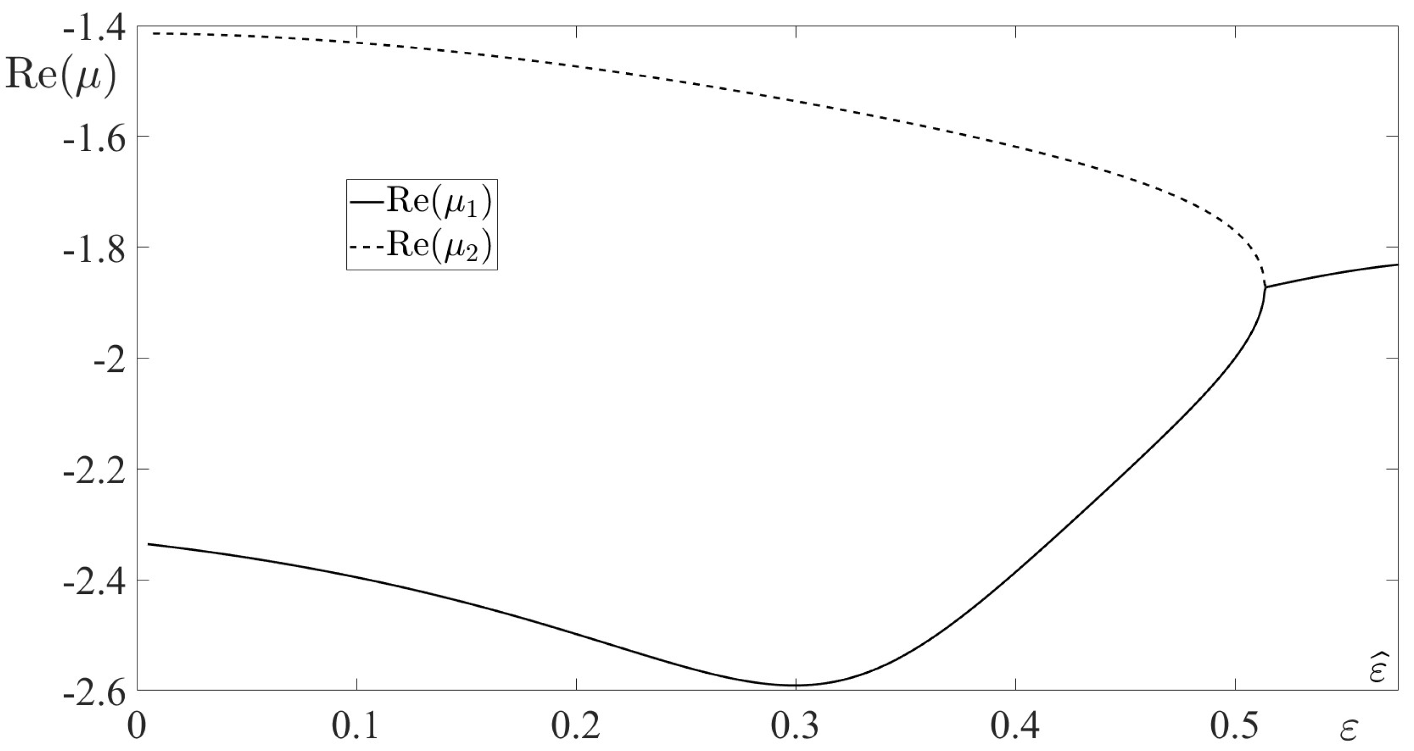
Figure 2.
Real part of .
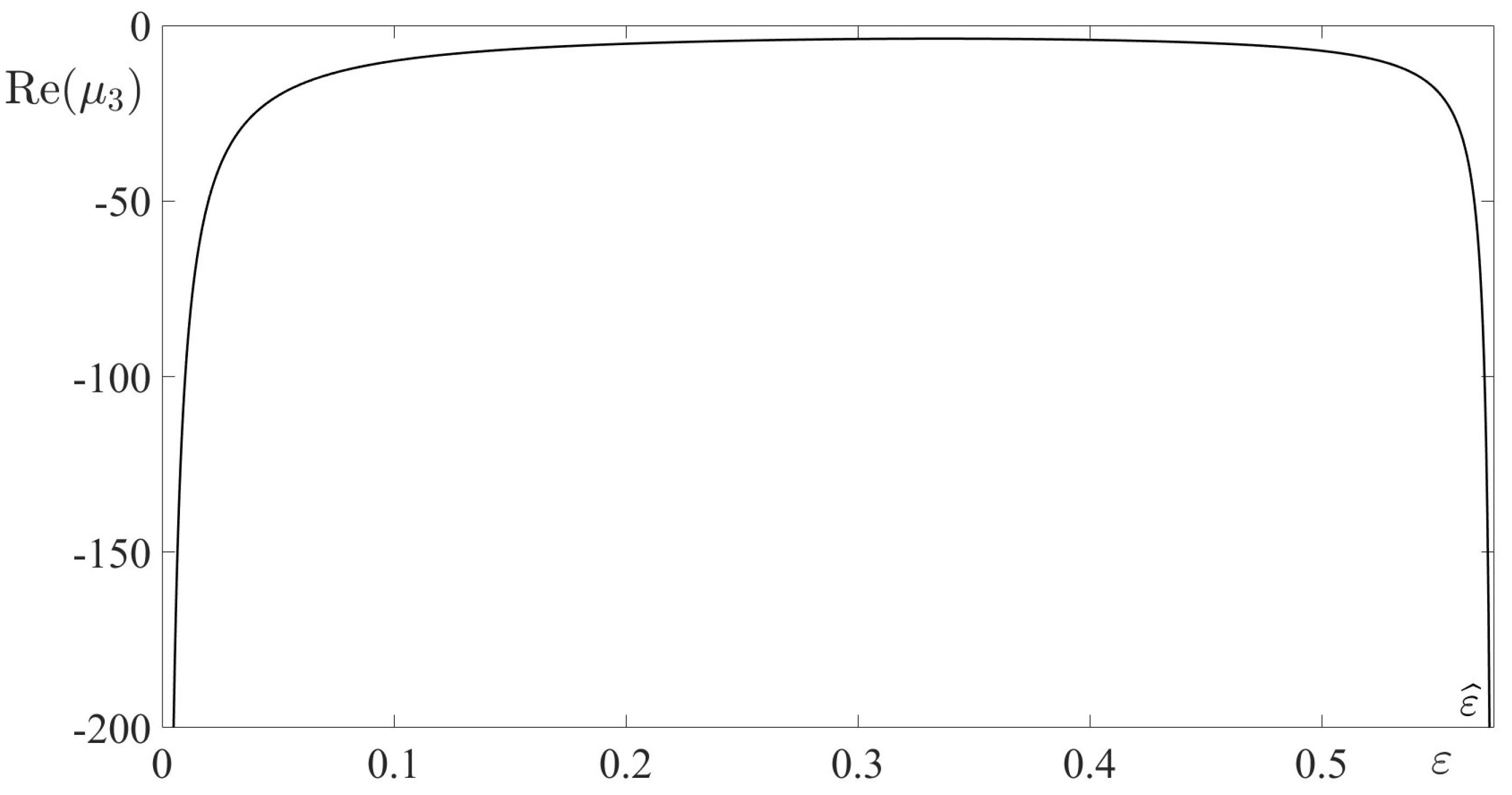
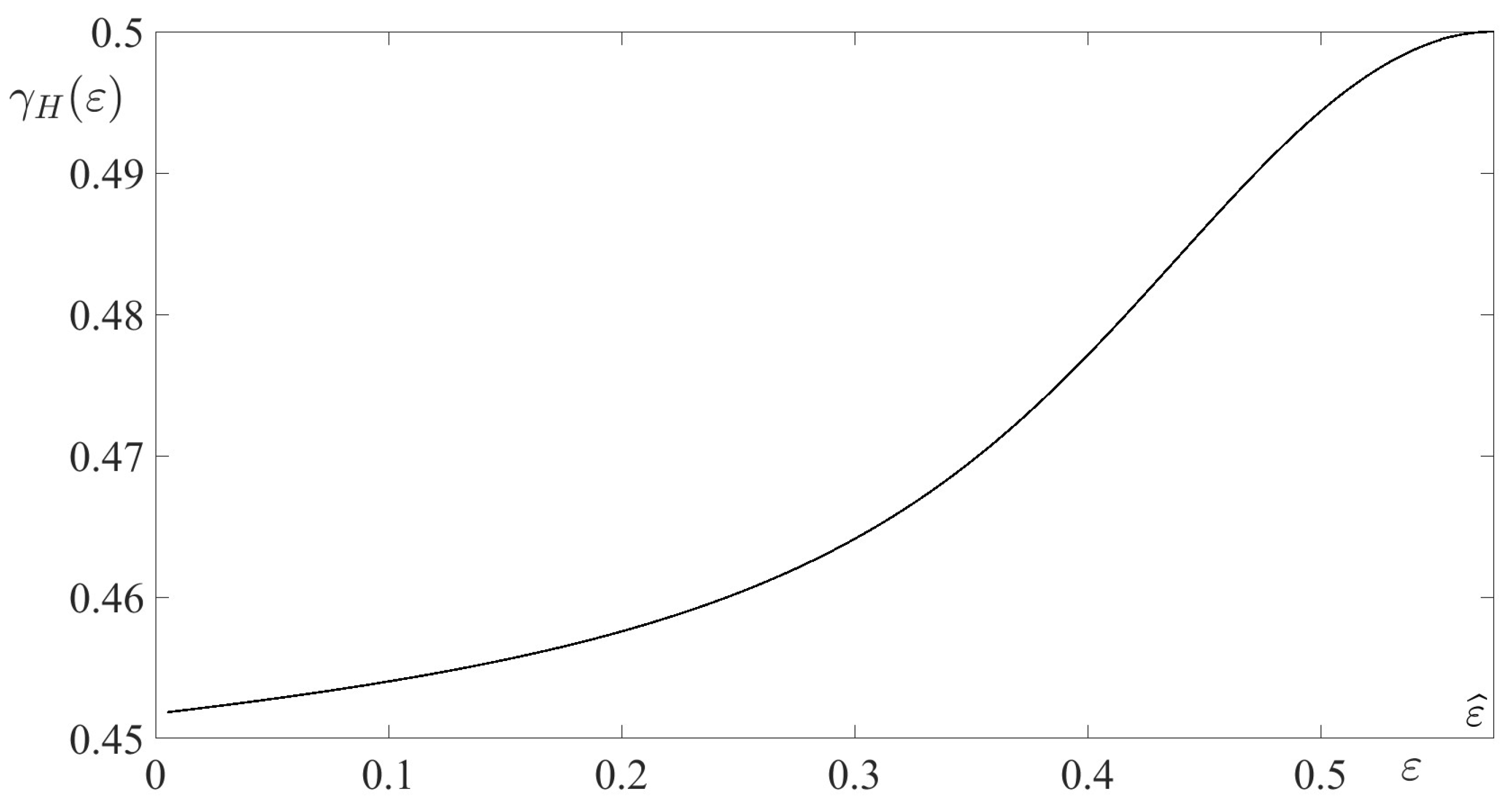
Figure 4.
Absolute errors of , .
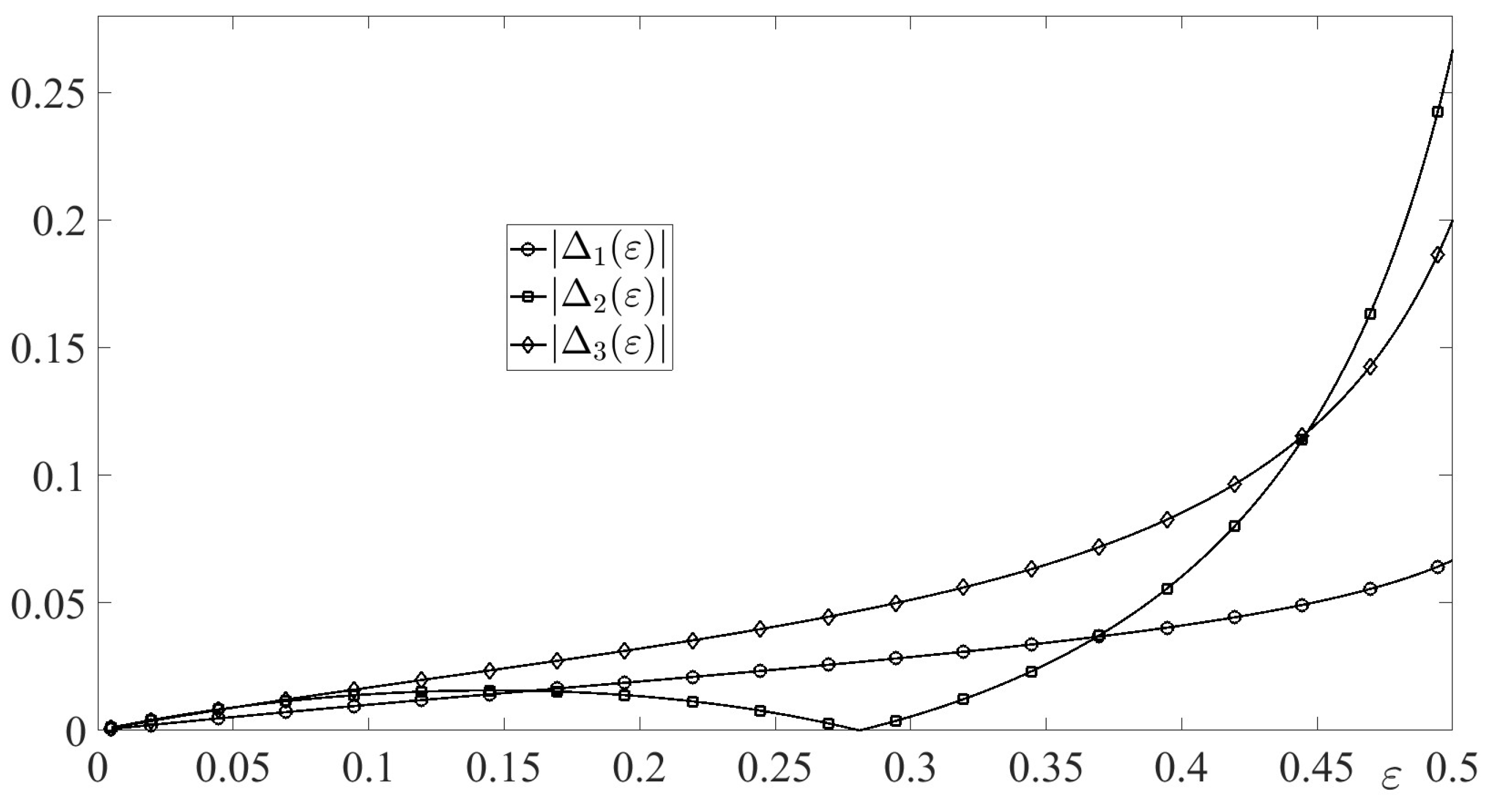
Figure 5.
Absolute errors of , .
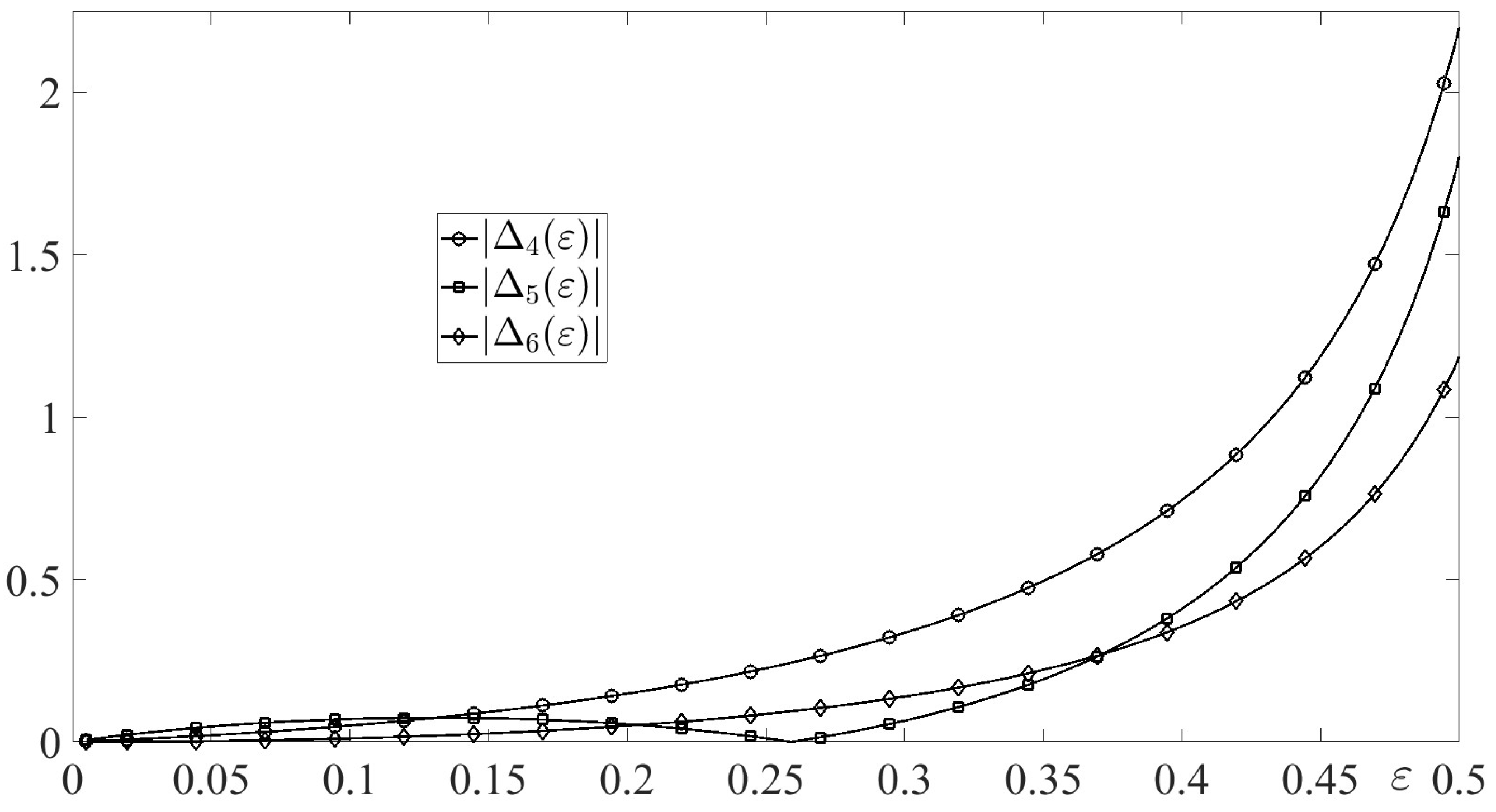
Figure 6.
Values of , .
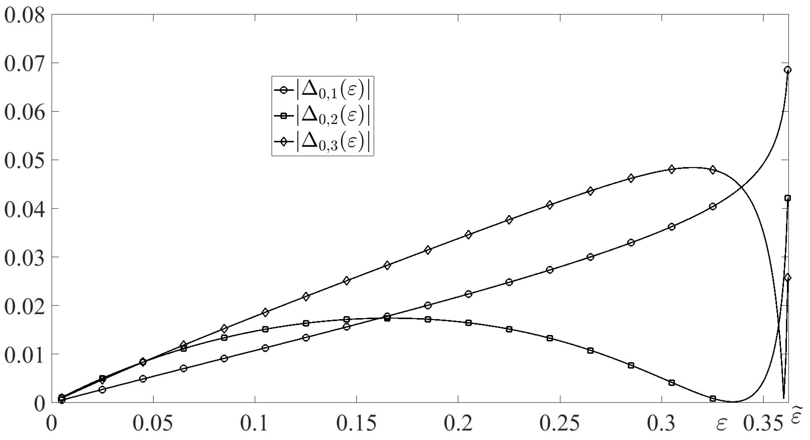
Figure 7.
Values of , .
Disclaimer/Publisher’s Note: The statements, opinions and data contained in all publications are solely those of the individual author(s) and contributor(s) and not of MDPI and/or the editor(s). MDPI and/or the editor(s) disclaim responsibility for any injury to people or property resulting from any ideas, methods, instructions or products referred to in the content. |
© 2025 by the authors. Licensee MDPI, Basel, Switzerland. This article is an open access article distributed under the terms and conditions of the Creative Commons Attribution (CC BY) license (http://creativecommons.org/licenses/by/4.0/).
Copyright: This open access article is published under a Creative Commons CC BY 4.0 license, which permit the free download, distribution, and reuse, provided that the author and preprint are cited in any reuse.


