Submitted:
13 December 2025
Posted:
15 December 2025
You are already at the latest version
Abstract
This paper examines the efficiency of a parallel version of an algorithm that utilizes the capabilities of the central processing unit (CPU) to calculate bifurcation diagrams of the Selkov fractional oscillator depending on the characteristic time scale. The parallel version of the algorithm is implemented in the ABMSelkovFracSim 2.0 software package written in Python, which also includes the Adams-Bashforth-Multon numerical algorithm, which enables one to find a numerical solution to the Selkov fractional oscillator that takes into account heredity or memory effects. The Selkov fractional oscillator is a system of nonlinear ordinary differential equations with Gerasimov-Caputo derivatives of fractional order variables and non-constant coefficients, which include a characteristic time scale parameter for matching the dimensions in the model equations. The paper evaluates the efficiency, speedup, and cost of the parallel algorithm, and presents a calculation of its optimal cost depending on the number of CPU threads. The optimal number of threads required to achieve maximum efficiency of the algorithm is determined. The TAECO approach was chosen to evaluate the efficiency of the parallel algorithm: T (execution time), A (acceleration), E (efficiency), C (cost), O (cost optimality index). Graphs of the efficiency characteristics of the parallel algorithm depending on the number of CPU threads are provided.
Keywords:
parallel algorithm
; efficiency
; speedup
; cost
; cost optimality index
; Selkov fractional oscillator
; Adams-Bashforth-Multon numerical algorithm
; bifurcation diagrams
; python
1. Introduction
Constructing bifurcation diagrams for various dynamic systems is of great practical importance, as it allows us to identify various regimes depending on changes in key parameters [1,2,3]. One such dynamic system, in our opinion, is the Selkov oscillator due to its important application in applied problems, for example, in biology for describing glycolytic reactions [4,5] or in seismology for describing microseisms [6]. From a mathematical perspective, the Selkov oscillator is a dynamic system consisting of two nonlinear first-order ordinary differential equations that describes various oscillatory regimes, including self-oscillations.
A generalization of the Selkov oscillator to the case of memory effects is the fractional Selkov oscillator [7]. Memory effects here indicate that the current state of the system depends on previous states, i.e., on its prehistory [8,9]. These effects can be described using the theory of fractional calculus using fractional derivatives [10,11,12]. In this case, the Selkov fractional oscillator is a nonlinear system of two ordinary differential equations of fractional orders. The introduction of fractional derivatives also entails the introduction of an additional parameter—a characteristic time scale—to match the dimensions of the right- and left-hand sides of the model equations, which is important in the study of dynamic regimes [13].
In the author’s work [7,14], a quantitative and qualitative analysis of the Selkov fractional oscillator was conducted in cases where the orders of the fractional derivatives were constant and where the characteristic time scale was chosen to be unity. Here, the system’s resting points were studied, the Adams-Bashforth-Multon numerical algorithm was implemented to construct oscillograms and phase trajectories, and regular and chaotic regimes were also investigated using the maximum Lyapunov exponents [34].
Further development of the Selkov fractional oscillator involved introducing derivatives of fractional order variables [16,17], which also resulted in non-constant coefficients in the model equations [18,19,20]. Quantitative and qualitative analyses were conducted using an adapted Adams-Bashforth-Multon algorithm, various oscillatory modes were investigated, and 2D and 3D bifurcation diagrams were constructed. These algorithms were implemented in the ABMSelkovFracSim 2.0 software package using the Python programming language and the PyCharm environment [21,22].
Constructing bifurcation diagrams is a rather computationally intensive task, as it requires repeatedly solving a system of fractional differential equations numerically. This leads to significant computational time expenditures [19,20]. Therefore, a parallel version of the bifurcation diagram calculation, depending on the characteristic time scale, was developed using Python tools . However, the parallel computation algorithm has not been studied for its efficiency depending on CPU threads. Therefore, in this paper, we examine its efficiency by addressing this gap and taking into account the available number of CPU threads, similar to the work [23].
The research plan in this article is structured as follows. In Section 2, we introduce some background information and define the key concepts used in the article. Section 3 presents the problem statement. Section 4 presents the Adams-Bashforth-Multon numerical algorithm for solving the problem. Section 5 describes a parallel algorithm implemented in the ABMSelkovFracSim 2.0 software suite for calculating bifurcation diagrams. Section 6 describes the parallel algorithm for constructing bifurcation diagrams. Section 7 analyzes the parallel algorithm’s performance depending on the number of CPU threads. Finally, we present conclusions on the parallel algorithm’s performance analysis.
2. Preliminaries
Definition 1.
The Gerasimov–Caputo fractional derivative of variable order of a function has the form [17]:
where is a function from the class , is the gamma function.
Remark 1.
Remark 2.
Definition 2.
A bifurcation diagram is a graphical representation of changes in the structure of solutions of a dynamic system when the parameters change. It shows how the stable and unstable states of the system change depending on the values of the parameters.
3. Statement of the Problem
Consider the following dynamic system:
where —solution functions; , , —functions from class ; —parameter with time dimension; —given constants; —current process time; —simulation time; —positive constants responsible for the initial conditions.
Operators of fractional variables of orders in the dynamic system (2) are understood in the sense of Gerasimov-Caputo (1). Following the work [19], we choose the following four types of functions and .
- 1.
- Constant fractional orderswhere are constant values of the fractional orders. Note that when , we arrive at the classical Selkov oscillator proposed in the work [4].
- 2.
- Cosine dependencewhere are the initial order values; are the oscillation amplitudes; are the oscillation frequencies; are the initial phases.
- 3.
- Exponential dependencewhere are the limiting values as , are the initial deviations, are the rates of exponential decay.
- 4.
- Linear dependencewhere are the initial values at , are the coefficients of linear decrease, is the lower boundary for computational stability.
Definition 3.
The dynamic system (2) will be called a Selkov fractional oscillator with variable coefficients and memory, or simply a Selkov fractional oscillator (SFO).
Remark 3.
4. Adams–Bashforth–Multon Method
To study the SFO (2), we use the Adams–Bashforth–Moulton numerical method (ABM) from the family of predictor–corrector methods. The ABM has been studied and discussed in detail in [28,29,30,31]. We adapt this method to solve the SFO (2). To do this on a uniform grid N with step , we introduce the functions , which will be determined by the Adams–Bashforth formula (predictor):
For the corrector (Adams–Moulton formula), we obtain
where , and weight coefficients in (3) are determined by the following formula:
Formulas (3) and (4) form the basis of a modified ABM method adapted for a fractional-order system (SFO) with variable exponents () and coefficients. The advantage of the ABM method is that it does not require solving nonlinear systems of equations at each step, significantly reducing computational costs. However, the main computational costs here are associated with storing the entire history (memory) of the vectors , which is typical for fractional integro-differentiation methods.
Remark 4.
The presented ABM method is explicit in its implementation, despite the use of the implicit Adams-Multon formula (4). Therefore, the ABM method is conditionally stable, like most explicit methods. It should also be noted that the order of accuracy of the ABM method is higher than that of the nonlocal explicit finite-difference scheme. The properties of the numerical ABM method (3), (4), convergence and stability issues can be studied in the work [18,19,20].
Based on the above Remark 4, the functions in the test examples for this article were chosen to be monotonically decreasing or not rapidly changing on the interval (0,1), and the sampling step was chosen small enough to prevent the solution from exhibiting unphysical oscillations or error growth.
5. ABMSelkovFracSim 2.0 Software Package
The paper [20] provides a detailed description of the ABM software package. We will focus on the module for calculating bifurcation diagrams (the Bifurcation analysis mode, Figure 1).
Figure 1 shows a screenshot of the main window of the Bifurcation Analysis mode. Here we see that this mode’s interface not only allows you to enter values for key FOS parameters and select one of four calculation methods depending on the function types , but also to set the range and step size for the key parameter . Furthermore, the required number of CPU threads can be selected, which are automatically determined for efficient parallel calculation of the bifurcation diagram.
Also, on the left side of the ABMSelkovFracSim 2.0 software interface in the Bifurcation Analysis mode, we see visualizations of the calculation results in the form of bifurcation diagrams and graphs of the functions . In Figure 1, the bifurcation diagram shows two ranges of parameter values, within which different dynamic FOS modes exist [19].
Remark 5.
It should be noted that the following useful information is displayed in the interface for the user of the ABMSelkovFracSim 2.0 software package: the time of calculation of the bifurcation diagram, the number of processed points in dynamics and the progress bar of the algorithm’s operation, and the possible presence of errors in the calculation.
Next, we will discuss in more detail the implementation of the parallel part of the bifurcation diagram calculation algorithm in the ABMSelkovFracSim 2.0 software.
6. Parallel Implementation of the Bifurcation Diagram Calculation Algorithm
Parallel implementation of algorithms is an important and relevant task in reducing their execution time. There are many approaches and technologies for parallelizing algorithms; these can be studied, for example, in the articles [32,33]. In this section, we will describe a parallelization method based on the built-in libraries of the Python programming language [21].
Due to the fact that the numerical algorithm ABM (3), (4) is practically impossible to parallelize due to the existence of true dependencies between the grid functions of the solutions and , we will parallelize multiple calculations using the ABM algorithm for each fixed value of the parameter from a given interval. That is, the operating principle of our parallel algorithm consists of the following steps: a separate independent process is created for each value of the parameter ; processes are executed in parallel on multiple processor cores; the results are collected after all calculations are completed. This is the classic "MapReduce" approach, where Map is the distribution of calculations across processes, and Reduce is the collection and merging of results. This approach is optimal for parametric studies, where each calculation is independent of the others.
To implement this approach, we will use Native Python Multiprocessing (Python Multiprocessing, ProcessPoolExecutor) technology from the Python Standard Library (Algorithm 1).
| Algorithm 1 Bifurcation analysis with parallel computing |
|
Remark 6.
Let’s highlight the key features of Algorithm 1:
- Data Parallelism: Each value of is processed independently.
- Process-based Parallelism: Processes (not threads) are used to bypass the Global Interpreter Lock (GIL).
- Master-Worker Pattern: The master process distributes tasks, and workers perform computations.
- Fault Tolerance: An error in one process does not affect others.
- Dynamic Load Balancing: ProcessPoolExecutor automatically distributes tasks.
We do not use other CPU parallelization technologies here for the following reasons. OpenMP is used for parallelization within a single process [34], which is not possible in our case. MPI is used for distributed computing on clusters, which is also not necessary in our case [35]. Threading: Threads in Python have a GIL and are not suitable for numerical calculations [36].
We now turn to the main goal of our article, to studying the efficiency of a parallel algorithm for calculating bifurcation diagrams.
7. Analysis of Algorithm Efficiency Based on Average Execution Time
All calculations in this article were performed on a computer with the following specifications: CPU — AMD Ryzen 7 7800X3D GHz cores; L2 cache 12 Mb & L3 cache 128 Mb; RAM — 64 Gb; GPU — NVIDIA GeForce RTX 5070 Ti, 16 Gb, 2300 MHz, ALU 8960.
Let us analyze the efficiency of the parallel computation algorithm of the ABMSelkovFracSim 2.0 software package in the mode of calculating and constructing a bifurcation diagram (Bifurcation analysis).
Since each new run of Bifurcation analysis will yield slightly different results for T — execution time in [sec.], and the number of experiments is finite, T can be considered a discrete random variable with some distribution function and mathematical expectation:
where i is the index of the Bifurcation analysis numerical experiment; L is the sample size; p is the number of CPU threads; N is the number of nodes in the uniform grid of the numerical method, i.e., the size of the input data.
Algorithm efficiency is the optimal ratio between computational speedup and the number of CPU threads, compared to the most efficient sequential version of the algorithm. However, when using a large number of CPU threads, the hardware and software limitations of parallelization’s acceleration efficiency become increasingly apparent. These limitations include the high time costs of parallelizing the task and reassembling all computational results [37], known as Amdahl’s law [23]. To represent various data on average execution time, we will use the following parameters in [sec]:
- — the execution time of a test example of size N required by the sequential Bifurcation analysis algorithm;
- — the execution time of a test example of size N required by the parallel Bifurcation analysis algorithm on a machine with CPU threads.
Let us calculate for different numbers of used CPU threads p in [units] with a step of 2.
To obtain efficiency estimates, data on average execution time are considered in terms of (TAECO) [38], applicable to algorithms: T (execution time), A (acceleration, speedup), E (efficiency), C (cost), O (cost-optimal indicator).
- — is the speedup of the algorithm, in [units], provided by the parallel version of the algorithm compared to the sequential one, and is calculated as follows:
- — is the efficiency of the algorithm, in [units/thread], of using a given number p of CPU threads and is defined by the ratio:moreover, by definition, the sequential algorithm has the greatest efficiency, . Therefore, for a parallel algorithm, it is better if .
- — is the cost of the algorithm, in [sec. × thread], which is determined by the product of a given number p of CPU threads and the T execution time of the parallel algorithm. The cost is determined by the ratio:
- — is the cost-optimal indicator (COI) of the algorithm, in [units × thread], characterized by a cost proportional to the complexity of the most efficient sequential algorithm:and the closer the value is to 1, the better, i.e., the cheaper the use of the parallel algorithm in terms of engaging CPU threads.
The calculations of efficiency indicators (5)-(9) and their visualization were performed in the MatlabR2025b computer mathematics system.
Example 1.
For the first example, we will choose the ABMSelkovFracCos method and the following parameter values for FOS (2): , .
In the Bifurcation analysis mode with all the same parameters, calculation method ABMSelkovFracCos, but with and step . To obtain the average execution time according to (5), we define , which will allow for smoother graphs for both average time and efficiency analysis.
Figure 2 presents the results of the efficiency analysis of the parallel Bifurcation analysis algorithm for the ABMSelkovFracCos method compared to its sequential counterpart. The results are presented as histograms for greater clarity. Parallelization, specific to this computer, allows achieving a maximum speedup of up to 8.5 times.
Figure 2 shows a dependence close to exponential: average execution time vs. number of CPU threads. Increasing the number of CPU threads at gives a greater performance gain compared to the sequential algorithm, but increasing the number of CPU threads at yields less and less performance gain. In the COI estimate, we see the opposite trend: the cost of using parallel algorithms does not change until around , and then increases linearly and proportionally to the growth in the number of CPU threads. Consequently, at we have the best efficiency coefficient of the parallel algorithm in relation to the cost of using the parallel algorithm , while obtaining a speedup of 6.75 times. As a result, we can say that the Bifurcation analysis mode is optimally parallelized on 7-8 threads, which, depending on the maximum number of CPUs of a particular computer, will allow running several copies of the ABMSelkovFracSim 2.0 software package itself for simultaneous work in several windows.
Example 2.
To evaluate the efficiency of the parallel version of the calculation algorithm, we will choose the ABMSelkovFracExp method.
We will select the parameter values from Example 1. To obtain the average time (5), the sample size is .
In the case of Test Example 2 for the ABMSelkovFracExp method, parallelization, for this particular computer, allows achieving a maximum speedup of times. The estimates for (Figure 3) have the same trends as for Test Example 1 (Figure 2). However, for , the cost of using parallel algorithms , and therefore , i.e., almost as effective as the sequential algorithm, with a 5-fold performance increase.
Example 3.
Let’s consider a parallel version of the algorithm for the ABMSelkovFracLinear method. For simplicity, we set .
The remaining parameter values are left unchange.
8. Conclusions
This article examines the effectiveness of a parallel algorithm for calculating bifurcation diagrams for the Selkov fractional oscillator, implemented using the standard Python library. The TAECO approach was chosen to evaluate the effectiveness of the parallel algorithm: T (execution time), A (acceleration), E (efficiency), C (cost), O (cost optimality index). Performance graphs were plotted for three ABM calculation methods: ABMSelkovFracCos, ABMSelkovFracExp, and ABMSelkovFracLinear. For these methods and a specific computer with 16 threads, approximately the same results were obtained. The effectiveness of the parallel algorithm is 8-9 times faster than that of the sequential version, while the optimal number of threads is 8 units. Therefore, the implementation of a parallel algorithm for calculating bifurcation diagrams of the fractional oscillator in the ABM software package is justified. Further development of research on this topic may be associated with the use of heterogeneous parallel programming structures, for example, CPU-GPU architecture, similar to the works [39,40].
Author Contributions
Conceptualization, R.P. and D.T.; methodology, R.P. and D.T.; software, R.P. and D.T.; validation, R.P. and D.T.; formal analysis, R.P. and D.T,; investigation, D.T.; data curation, D.T.; writing—original draft preparation, R.P. and D.T.; writing—review and editing, R.P.; visualization, D.T.; supervision, R.P. All authors have read and agreed to the published version of the manuscript.
Funding
The work was carried out within the framework of the state assignment of IKIR FEB RAS (reg. No. 124012300245-2).
Data Availability Statement
The original contributions presented in this study are included in the article. Further inquiries can be directed to the corresponding author.
Conflicts of Interest
The authors declares no conflicts of interest.
Abbreviations
The following abbreviations are used in this manuscript:
| CPU | Central Processing Unit |
| SFO | Selkov Fractional Oscillator |
| ABM | Adams–Bashforth–Moulton Numerical Method |
| GPU | Graphics Processing Unit |
| RAM | Random Access Memory |
| GIL | Global Interpreter Lock |
| OpenMP | Open Multi-Processing |
| MPI | Message Passing Interface |
References
- Sinet, S.; Bastiaansen, R.; Kuehn, C.; von der Heydt, A. S.; Dijkstra, H. A. Approximating the bifurcation diagram of weakly and strongly coupled leading-following systems. Chaos: An Interdisciplinary Journal of Nonlinear Science 2025, 35. [Google Scholar] [CrossRef]
- Li, X.; Liu, G.; Liu, J.; Chen, Y. Unveiling Pseudo-Period-Tripling Bifurcations in Nonlinear Dynamical Systems. International Journal of Bifurcation and Chaos 2025, 35, 2550156. [Google Scholar] [CrossRef]
- Gong, R.; Xu, J.; Liu, T.; Qin, Y.; Wei, Z. Bifurcation and Chaos in DCM Voltage-Fed Isolated Boost Full-Bridge Converter. Electronics 2025, 14, 260. [Google Scholar] [CrossRef]
- Sel’kov, E.E. Self-Oscillations in Glycolysis 1. A Simple Kinetic Model. European Journal of Biochemistry 1968, 4, 79–86. [Google Scholar] [CrossRef]
- Dhatt, S.; Chaudhury, P. Study of oscillatory dynamics in a Selkov glycolytic model using sensitivity analysis. Indian Journal of Physics 2025, 96, 1649–1654. [Google Scholar] [CrossRef]
- Makovetsky, V. I.; Dudchenko, I. P.; Zakupin, A. S. Auto oscillation model of microseism’s sources. Geosist. Pereh. Zon 2017, 4, 37–46. [Google Scholar]
- Parovik, R.I. Studies of the fractional Selkov dynamical system for describing the self-oscillatory regime of microseisms. Mathematics 2022, 10, 4208. [Google Scholar] [CrossRef]
- Volterra, V. Functional Theory, Integral and Integro-Differential Equations; Dover Publications: Mineola, USA, 2005. [Google Scholar]
- Nyerere, N.; Edward, S. Modeling Chlamydia transmission with caputo fractional derivatives: exploring memory effects and control strategies. Modeling Earth Systems and Environment 2025, 11, 307. [Google Scholar] [CrossRef]
- Nakhushev, A.M. Fractional Calculus and Its Applications; Fizmatlit: Moscow, Russia, 2003. [Google Scholar]
- Kilbas, A.A.; Srivastava, H.M.; Trujillo, J.J. Theory and Applications of Fractional Differential Equations; Elsevier: Amsterdam, Netherlands, 2006. [Google Scholar]
- García, J. J. R.; Escalante-Martínez, J. E.; Rojano, F. A. G.; Fuentes, J. C. M.; Torres, L. Advances in Fractional Calculus; Springer: Charm, Switzerland, 2025. [Google Scholar] [CrossRef]
- Aguilar, J. F. G.; Córdova-Fraga, T.; Tórres-Jiménez, J.; Escobar-Jiménez, R. F.; Olivares-Peregrino, V. H.; Guerrero-Ramírez, G. V. Nonlocal Transport Processes and the Fractional Cattaneo-Vernotte Equation. Mathematical Problems in Engineering 2016, 2016, 7845874. [Google Scholar] [CrossRef]
- Parovik, R. I.; Rakhmonov, Z.; Rakhim Zunnunov, R. Study of Chaotic and Regular Modes of the Fractional Dynamic System of Selkov. EPJ Web of Conferences 2021, 254, 02014. [Google Scholar] [CrossRef]
- Zhou, S.; Zhang, Q.; He, S.; Zhang, Y. What is the lowest cost to calculate the Lyapunov exponents from fractional differential equations? Nonlinear Dynamics 2025, 113, 1–47. [Google Scholar] [CrossRef]
- Sun, H.; Chang, A.; Zhang, Y.; Chen, W. A Review on Variable-Order Fractional Differential Equations: Mathematical Foundations, Physical Models, Numerical Methods and Applications. Fractional Calculus and Applied Analysis 2019, 22, 27–59. [Google Scholar] [CrossRef]
- Patnaik, S.; Hollkamp, J.P.; Semperlotti, F. Applications of variable-order fractional operators: a review. Proceedings of the Royal Society A: Mathematical, Physical and Engineering Sciences 2020, 476, 20190498. [Google Scholar] [CrossRef]
- Parovik, R.I. Selkov’s Dynamic System of Fractional Variable Order with Non-Constant Coefficients. Mathematics 2025, 13, 372. [Google Scholar] [CrossRef]
- Parovik, R.I. Study of dynamic modes of fractional Selkov oscillator with variable coefficients using bifurcation diagrams. Comput Math Model 2025. [Google Scholar] [CrossRef]
- Parovik, R. I. ABMSelkovFracSim 2.0 software package for quantitative and qualitative analysis of the Selkov fractional oscillator. Vestnik KRAUNC. Fiz.-mat. nauki 2025, 53, 75–92. [Google Scholar]
- Shaw, Z.A. Learn Python the Hard Way; Addison-Wesley Professional: Boston, USA, 2024. [Google Scholar]
- Van Horn, B.M.; Nguyen, Q. Hands-On Application Development with PyCharm: Build Applications Like a Pro with the Ultimate Python Development Tool; Packt Publishing Ltd.: Birmingham, United Kingdom, 2023. [Google Scholar]
- Tverdyi, D. A. An Analysis of the Computational Complexity and Efficiency of Various Algorithms for Solving a Nonlinear Model of Radon Volumetric Activity with a Fractional Derivative of a Variable Order. Computation 2025, 13, 252. [Google Scholar] [CrossRef]
- Novozhenova, O.G. Life And Science of Alexey Gerasimov, One of the Pioneers of Fractional Calculus in Soviet Union. Fractional Calculus and Applied Analysis 2017, 20, 790–809. [Google Scholar] [CrossRef]
- Caputo, M.; Fabrizio, M. On the notion of fractional derivative and applications to the hysteresis phenomena. Meccanica 2017, 52, 3043–3052. [Google Scholar] [CrossRef]
- Parovik, R. I. Qualitative analysis of Selkov’s fractional dynamical system with variable memory using a modified Test 0-1 algorithm. Vestnik KRAUNC. Fiz.-mat. nauki 2023, 45, 9–23. [Google Scholar] [CrossRef]
- Parovik, R.I. Selkov dynamic system with variable heredity for describing Microseismic regimes. In Solar-terrestrial relations and physics of earthquake precursors: proceedings of the XIII international conference; Dmitriev, A., Lichtenberger, J., Mandrikova, O., Nahayo, E., Eds.; Nature Switzerland: Cham, Switzerland, 2023; pp. 166–178. [Google Scholar] [CrossRef]
- Diethelm, K.; Ford, N.J.; Freed, A.D. A Predictor-Corrector Approach for the Numerical Solution of Fractional Differential Equations. Nonlinear Dynamics 2002, 29, 3–22. [Google Scholar] [CrossRef]
- Yang, C.; Liu, F. A computationally effective predictor-corrector method for simulating fractional order dynamical control system. ANZIAM Journal 2005, 47, 168. [Google Scholar] [CrossRef]
- Garrappa, R. Numerical solution of fractional differential equations: A survey and a software tutorial. Mathematics 2018, 6, 16. [Google Scholar] [CrossRef]
- Naveen, S.; Parthiban, V. Qualitative analysis of variable-order fractional differential equations with constant delay. Mathematical Methods in the Applied Sciences 2024, 47, 2981–2992. [Google Scholar] [CrossRef]
- Sino, M.; Domazet, E. Scalable Parallel Processing: Architectural Models, Real-Time Programming, and Performance Evaluation. Eng. Proc. 2025, 104, 60. [Google Scholar] [CrossRef]
- Meng, X.; He, X.; Hu, C.; et al. A Review of Parallel Computing for Large-scale Reservoir Numerical Simulation. Arch Computat Methods Eng 2025, 32, 4125–4162. [Google Scholar] [CrossRef]
- Zhou, X.; Wang, C. Research on optimization of data mining algorithm based on OpenMP. SPIE 2025, 13560, 850–857. [Google Scholar] [CrossRef]
- Himstedt, K. Multiple execution of the same MPI application: exploiting parallelism at hotspots with minimal code changes. GEM-International Journal on Geomathematics 2025, 16, 1–28. [Google Scholar] [CrossRef]
- Wicaksono, D.; Soewito, B. Application of the multi-threading method and Python script for the network automation. Journal of Syntax Literate 2024, 9. [Google Scholar]
- Rauber, T.; Runger, G. Parallel Programming for Multicore and Cluster Systems; Springer: New York, USA, 2013. [Google Scholar]
- Al-hayanni, M. A. N.; Xia, F.; Rafiev, A.; Romanovsky, A.; Shafik, R.; Yakovlev, A. Amdahl’s Law in the Context of Heterogeneous Many-core Systems-ASurvey. IET Computers & Digital Techniques 2020, 14, 133–148. [Google Scholar] [CrossRef]
- Skorych, V.; Dosta, M. Parallel CPU–GPU computing technique for discrete element method. Concurrency and Computation: Practice and Experience 2022, 34, e6839. [Google Scholar] [CrossRef]
- Alaei, M.; Yazdanpanah, F. A survey on heterogeneous CPU–GPU architectures and simulators. Concurrency and Computation: Practice and Experience 2025, 37, e8318. [Google Scholar] [CrossRef]
Figure 1.
A screenshot of the main window of the ABMSelkovFracSim 2.0 software package in the Bifurcation Analysis mode
Figure 1.
A screenshot of the main window of the ABMSelkovFracSim 2.0 software package in the Bifurcation Analysis mode
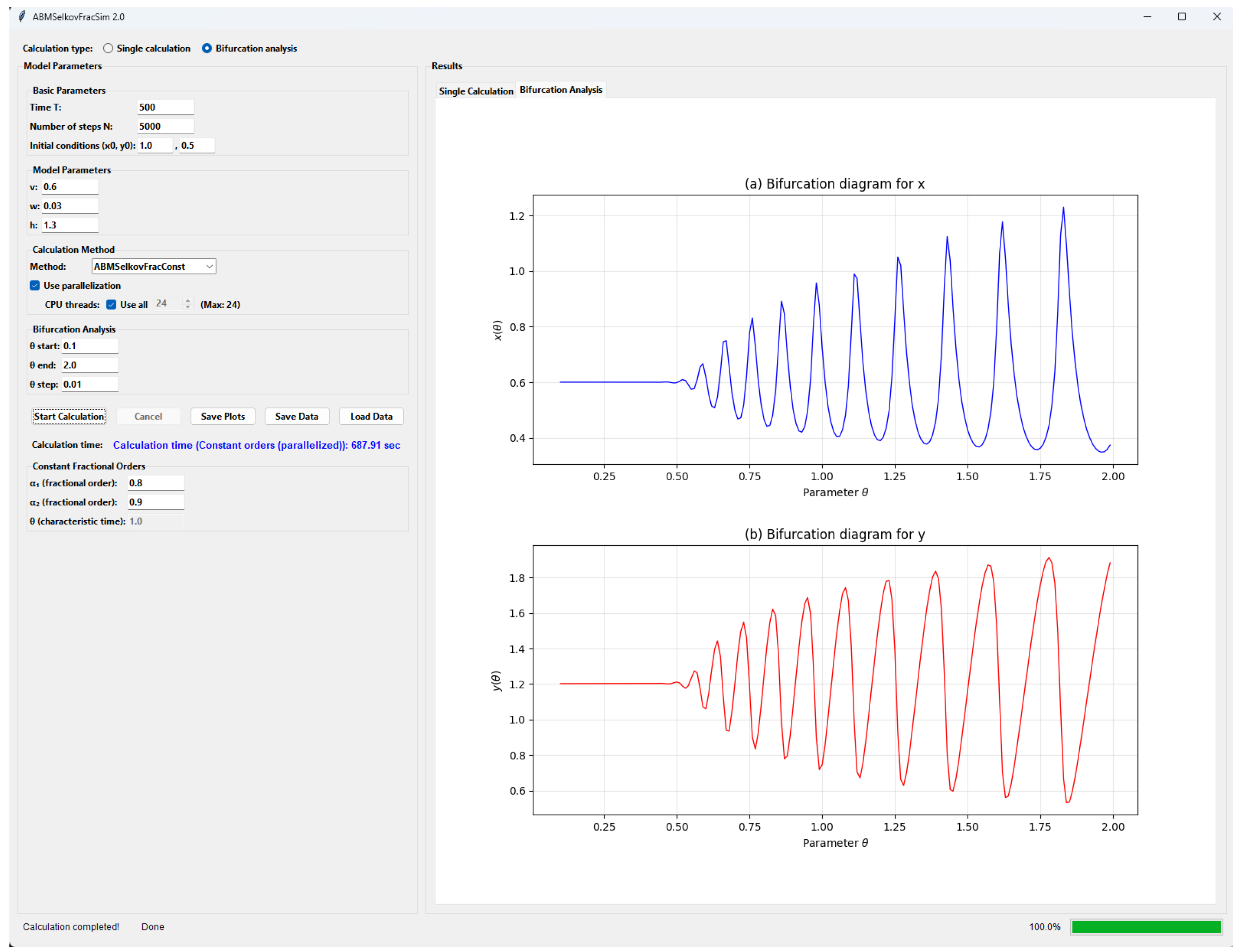
Figure 2.
Average execution time and efficiency estimation of a parallel algorithm implementing Bifurcation analysis (Example 1): (a) - , (b) - , (c) - , (d) -
Figure 2.
Average execution time and efficiency estimation of a parallel algorithm implementing Bifurcation analysis (Example 1): (a) - , (b) - , (c) - , (d) -
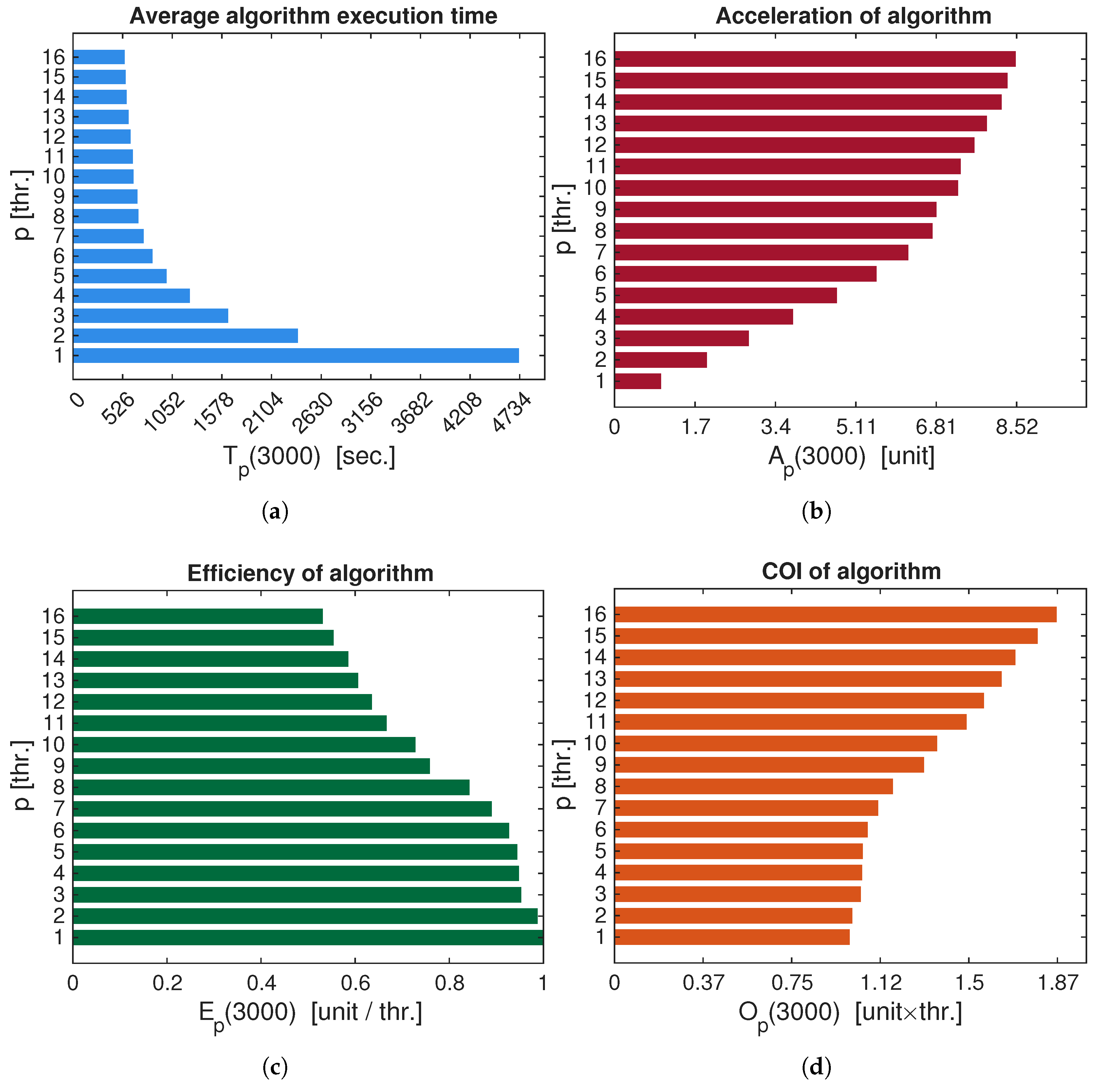
Figure 3.
Average execution time and efficiency estimation of a parallel algorithm implementing Bifurcation analysis (Example 2): (a) - , (b) - , (c) - , (d) -
Figure 3.
Average execution time and efficiency estimation of a parallel algorithm implementing Bifurcation analysis (Example 2): (a) - , (b) - , (c) - , (d) -
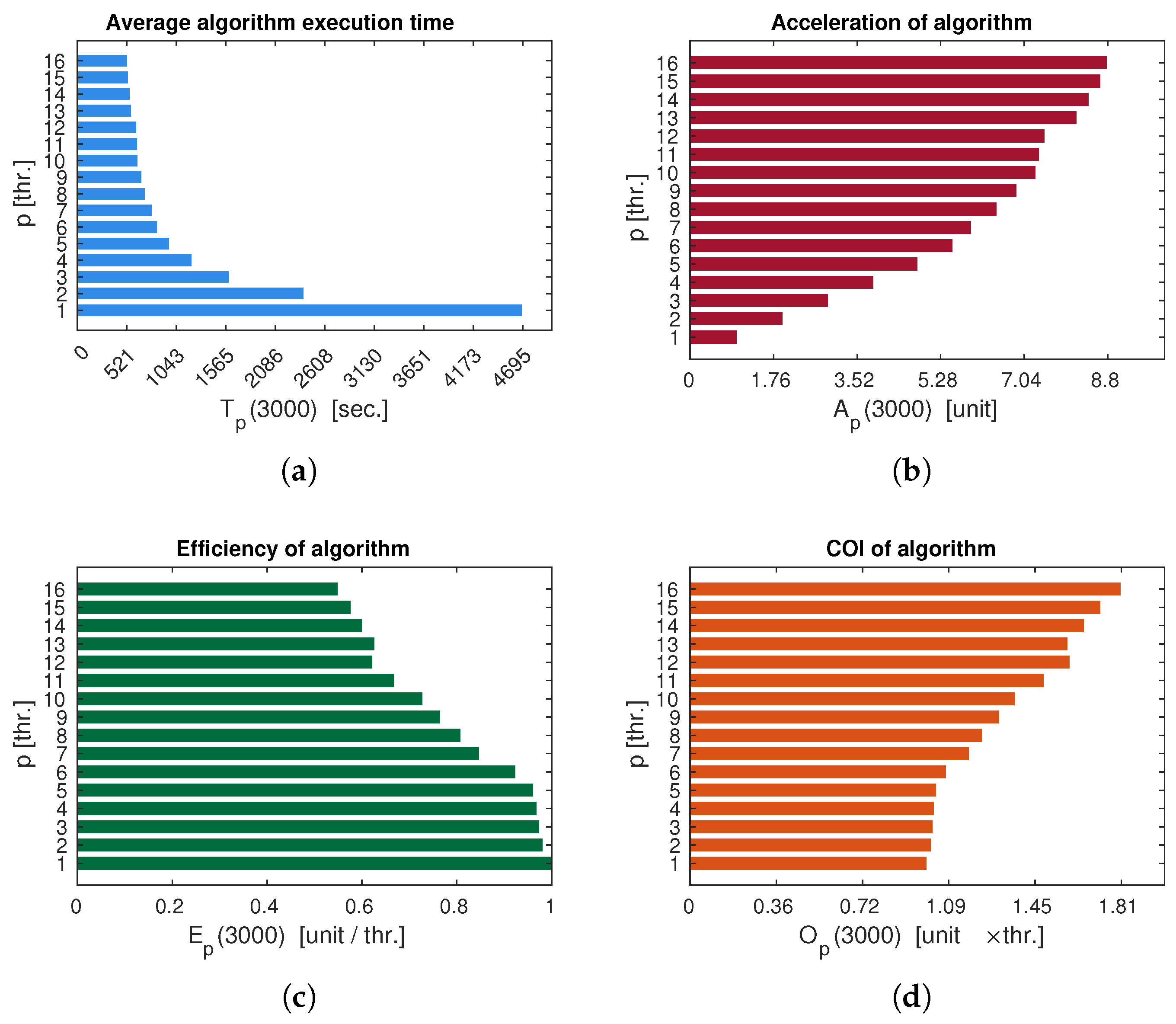
Figure 4.
Average execution time and efficiency estimation of a parallel algorithm implementing Bifurcation analysis (Example 3): (a) - , (b) - , (c) - , (d) -
Figure 4.
Average execution time and efficiency estimation of a parallel algorithm implementing Bifurcation analysis (Example 3): (a) - , (b) - , (c) - , (d) -
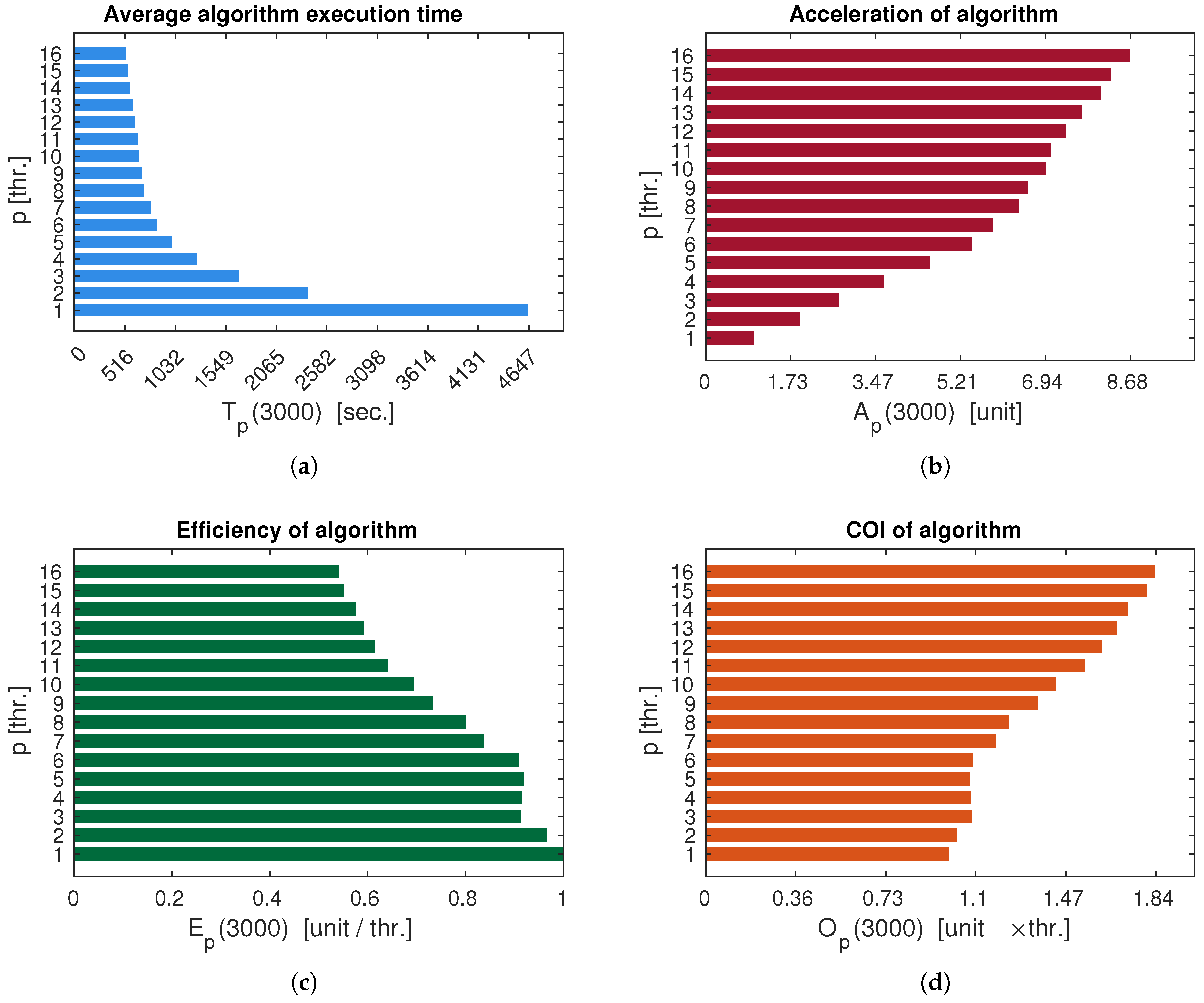

Table 1.
Average execution time of the test Example 1 with a varying number of CPU threads.
| p, | , |
|---|---|
| 1 | 4734 |
| 2 | 2392 |
| 3 | 1653 |
| 4 | 1245 |
| 5 | 1000 |
| 6 | 849 |
| 7 | 757 |
| 8 | 700 |
| 9 | 691 |
| 10 | 648 |
| 11 | 643 |
| 12 | 619 |
| 13 | 598 |
| 14 | 575 |
| 15 | 567 |
| 16 | 555 |
Table 2.
Average execution time of the test Example 2 with a varying number of CPU threads.
| p, | , |
|---|---|
| 1 | 4695 |
| 2 | 2390 |
| 3 | 1605 |
| 4 | 1210 |
| 5 | 976 |
| 6 | 846 |
| 7 | 790 |
| 8 | 725 |
| 9 | 681 |
| 10 | 643 |
| 11 | 637 |
| 12 | 627 |
| 13 | 575 |
| 14 | 558 |
| 15 | 542 |
| 16 | 533 |
Table 3.
Average execution time of the test Example 3 with a varying number of CPU threads.
| p, | , |
|---|---|
| 1 | 4647 |
| 2 | 2399 |
| 3 | 1692 |
| 4 | 1266 |
| 5 | 1009 |
| 6 | 849 |
| 7 | 790.44 |
| 8 | 723 |
| 9 | 703 |
| 10 | 666 |
| 11 | 656 |
| 12 | 628 |
| 13 | 602 |
| 14 | 574 |
| 15 | 559 |
| 16 | 535 |
Disclaimer/Publisher’s Note: The statements, opinions and data contained in all publications are solely those of the individual author(s) and contributor(s) and not of MDPI and/or the editor(s). MDPI and/or the editor(s) disclaim responsibility for any injury to people or property resulting from any ideas, methods, instructions or products referred to in the content. |
© 2025 by the authors. Licensee MDPI, Basel, Switzerland. This article is an open access article distributed under the terms and conditions of the Creative Commons Attribution (CC BY) license (http://creativecommons.org/licenses/by/4.0/).
Copyright: This open access article is published under a Creative Commons CC BY 4.0 license, which permit the free download, distribution, and reuse, provided that the author and preprint are cited in any reuse.


