Submitted:
12 December 2025
Posted:
15 December 2025
You are already at the latest version
Abstract
Accurately determining actual energy consumption is essential for guiding technological developments in the transport sector, assessing vehicle development outcomes, and designing effective energy and climate policies. Although laboratory driving cycles such as the WLTP provide standardized benchmarks, they do not reflect the complex interactions between human behavior, environmental conditions, and vehicle dynamics under real-world operating conditions. This article presents an integrated framework for assessing long-term, actual energy carriers consumption in four main vehicle categories: internal combustion engine vehicles (ICEVs), hybrid electric vehicles (HEVs), hydrogen fuel cell electric vehicles (H2EVs), and battery electric vehicles (BEVs). The entire discussion here is based on the results of data analysis from natural operation using the so-called vehicle energy footprint. This framework provides a method for determining the average energy carriers consumption for each group of vehicles with the specified drivetrains. This information formed the basis for assessing the total energy demand for the operation of the analyzed vehicle types in normal operation. The simulations show that among mid-range passenger vehicles, ICEVs are the most energy-intensive in normal operation, followed by H2EVs, HEVs, and BEVs the least. The study highlights the methodological challenges and implications of accurately quantifying energy consumption. The presented method for assessing energy demand in vehicle operation can be useful for manufacturers, consumers, fleet operators, and policymakers, particularly in terms of energy efficiency, emission reduction, and public health protection.
Keywords:
car natural operation
; long-term
; energy consumption
; assessing method
1. Introduction
Energy “consumption” in the transport sector is a key determinant of both economic performance and environmental impact.
For internal combustion engine vehicles (ICEVs), fuel consumption has long served as a primary indicator of vehicle efficiency. However, as hybrid electric vehicles (HEVs), hydrogen fuel cell electric vehicles (H2EVs), and battery electric vehicles (BEVs) gain prominence, the scope of efficiency assessment must expand to encompass multiple energy carriers—liquid fuels, hydrogen, and electricity—under real-world operating conditions.
Despite decades of standardization efforts, discrepancies persist between laboratory-derived and real-world energy consumption. Standardized procedures such as the New European Driving Cycle (NEDC) and the Worldwide Harmonized Light Vehicles Test Procedure (WLTP) are designed for comparability, not representativeness. Empirical data consistently indicate that real-world energy use exceeds laboratory values [1] due to factors including driver behavior, traffic congestion, vehicle load, climatic variability, and topographic conditions.
This paper addresses the challenge of accurately quantifying real-world energy consumption through the long-term monitoring of vehicles in natural operation, integrating conventional and alternative powertrain technologies within a unified analytical framework.
The challenge is determining energy demand under real-world vehicle operating conditions. Therefore, this article presents a unique method for assessing this demand under long-term, natural vehicle use.
Accurately assessing energy demand under natural conditions (i.e., “everyday” vehicle use over extended periods) is essential for key stakeholders, including:
- Vehicle fleet operators who rely on precise data on energy demand to effectively manage transport, and fuel-efficient fleet management can reduce the costs of purchasing energy carriers by up to 20% [4].
- Individual consumers who are looking for vehicles whose use will reduce operating costs, and the discrepancy between energy demand in laboratory conditions and real life [2] may lead to a change in purchasing priorities, as many consumers base their purchasing decisions on official energy demand indicators [5].
- Vehicle manufacturers, for whom energy demand is a key design parameter that influences consumer choices and regulatory compliance. (CAFE) [6].
As transport decarbonization accelerates, precise assessment of real-world energy use across all propulsion technologies becomes indispensable for evidence-based policy design.
- ICEVs primarily emit CO2, NOₓ, SOₓ, CO, VOCs, and particulate matter (PM2.5, PM10) [9].
- HEVs mitigate these emissions partially through regenerative braking and hybrid power management, but remain
- BEVs exhibit zero tailpipe emissions but shift the environmental burden to electricity generation and battery manufacturing. The real-world electricity consumption of BEVs depends on driving patterns, temperature, battery aging, and auxiliary loads (e.g., heating, cooling) [10].
- H2EVs produce only water vapor at the point of use; however, their total life-cycle emissions depend on hydrogen production pathways—currently dominated by steam methane reforming [11].
According to the World Health Organization (WHO) [12] and European Environment Agency (EEA) [13], air pollution from vehicle emissions contributes to millions of premature deaths annually, particularly in urban areas with high traffic density. The OECD [14] estimates that air pollution–related diseases impose a global economic burden exceeding 2.5% of GDP. Therefore, accurate quantification of energy consumption and associated emissions is not only a technical challenge but a prerequisite for public health protection.
The transition to sustainable mobility requires a robust, harmonized methodology for long-term, real-world energy consumption assessment. Traditional on-board fuel flow measurement must be complemented by data logging systems capable of integrating multiple energy carriers—liquid fuels, hydrogen, and electricity—within a single analytical framework.
Such datasets enable the comparison of vehicles not merely by theoretical efficiency but by effective energy intensity under actual usage conditions, expressed in MJ/km or kWh/km after well-to-wheel normalization. This holistic approach aligns with life-cycle analysis (LCA) principles and supports a more accurate evaluation of total environmental impact.
Long-term real-world energy consumption assessment is fundamental to achieving transparency, efficiency [15], and sustainability [16,17,18,19]. In the transport sector it enables:
- Evidence-based vehicle design and regulatory compliance;
- Informed consumer decision-making;
- Optimization of fleet operations and logistics;
- Development of coherent, data-driven public policy.
The accurate determination of energy consumption across ICEV, HEV, H2EV, and BEV categories is indispensable for quantifying true progress toward transport decarbonization. Future research should focus on integrating telematics, on-board diagnostics, and life-cycle energy modeling to establish a universal framework for real-world energy performance evaluation.
2. Objectives of This Study
The purpose of this paper is to present a new method for assessing long-term fuel consumption during normal vehicle operation.
Traditionally, the main methods used to assess fuel consumption [7] in real-world conditions [3] are:
- Full-tank method (“tank-to-tank”). This is a simple and relatively accurate method used by drivers and fleet operators. Advantages: Simple and reliable for assessing fuel consumption over relatively long distances (high mileage). Disadvantages: Does not provide real-time fuel consumption changes.
- On-board computer readings. Most modern vehicles have an on-board computer that displays average and instantaneous fuel consumption. Advantages: Immediate results. Useful for correcting driving habits. Provides both average and instantaneous fuel consumption. Disadvantages: May have a margin of error of 5-10%. Older vehicles may not have this feature.
- OBD-II diagnostics + mobile apps. If the vehicle has an OBD-II port (on-board diagnostics), it is possible to use a Bluetooth scanner with apps to monitor fuel consumption in real time. Advantages: Provides precise, real-time fuel delivery data from the engine control unit. Allows for tracking additional parameters (e.g., engine load, temperature, or throttle position). Disadvantages: Requires additional hardware and configuration. Accuracy depends on sensor calibration.
- Long-term statistical analysis (fleet management). For commercial fleets, fuel consumption is analyzed over a long period of time based on: fuel purchase records (e.g., receipts, invoices). Odometer readings (from GPS or tachograph). Driving conditions (city driving, highway driving, cargo). Advantages: Best for fleet management. Helps detect inefficient solutions. Disadvantages: Requires consistent data collection.
- Real-world driving emissions (RDE) testing using portable emission measurement systems (PEMS). Used in regulatory and scientific studies. this method involves: Installing a portable emissions analyzer (PEMS) on the vehicle. Measuring real-time fuel consumption under real-world driving conditions. Pros: Most accurate real-world method. Cons: Expensive. used mainly in professional research.
However, in addition to the methods mentioned above, there are likely other methods for assessing fuel consumption (energy demand) that are not widely described in the literature, especially when it comes to the crucial topic of collecting operational data. There are websites offering the ability for direct vehicle users to record a wide variety of operational data. Statistically speaking, this appears to be a very important source of data, which can also be further processed using appropriate mathematical methods. This data has the undeniable advantage of being authentic. The use of such data through appropriate mathematical methods is the main topic of this study. It uses operational data widely available on the spritmonitor.de website [20].
The mathematical method used to develop the data and analyze the obtained results is the theory of cumulative fuel consumption and the vehicle energy footprint derived from it – the application of this theory will be presented in the following chapters.
3. Cumulative energy demand of cars
Before we move on to the actual assessment of the energy demand for vehicle traffic during their operational use, we will present how to use data from spritmonitor.de to create an indicator such as fuel economy.
Among the methods for assessing energy demand, and traditionally fuel consumption, of engines in long-term, natural vehicle operation, the most commonly used method to date is the “full tank” method, also known as “tank-to-tank.” However, there are two basic variations of this method: one reports fuel consumption in units of volume of fuel consumed relative to distance traveled (usually dm³ per 100 km). The other reports the distance traveled on a given volume of fuel (usually miles per gallon).
In the EU, the traditional fuel economy metric is fuel economy (FE), expressed in dm³/100 km (liters/100 km or l/100 km). Considering different drive types, this metric can also be expressed in kg/100 km (e.g., for hydrogen-powered vehicles) or kWh/100 km for electric vehicles (it is clear that after the introduction of new energy carriers to power vehicle drive systems, the fuel economy indicator has been adjusted accordingly by society as a whole).
The procedure for constructing the FE indicator is presented here using data from spritmonitor.de. This data is the result of long-term. natural operation of a mid-size hydrogen-powered passenger car (H2EV). In the spritmonitor.de database. the vehicle was assigned the number 1195603 (just like other vehicles that are assigned specific numbers in the spritmonitor database - they have nothing to do with the vehicle’s VIN or registration number). This data is presented in Table 1.
The data in the “Data”. “Tachostand”. “Distance” and “Menge” columns comes directly from the spritmonitor.de database. The data in the remaining columns is calculated based on data from the spritmonitor.de database.
Analyzing the presented data. it can be seen that it covers mileage ranging from 33,985 km recorded on August 15. 2020. to 44,797 km recorded on August 26. 2021. Therefore. the data covers a trip distance of 10,802 km traveled in one year. This data can undoubtedly be classified as operational data from the vehicle’s long-distance natural operation.
Analyzing the data further. the following results can be presented. By the assumptions that
Fi – i-th refueling.
tdi – mileage to Fi.
the fuel economy (FE) can be expressed as:
The achieving results are presented in column FE the Table 1.
As can be seen. the data are statistical in nature. Allowing for a comprehensive statistical analysis. If all refueling are treated as one set, then the statistical analysis is obtained. Such an analysis was conducted. and the results are presented in Table 2.
With statistical analysis data available, it is possible to present both the mean (FE(AV)) and the ranges of data variability as a function of vehicle mileage: from Mean - Standard Deviation (FE(AV-SD)) to Mean + Standard Deviation (FE(AV+SD)).
These values are marked in Figure 1.
Although this data presentation seems to be common practice, it seems more interesting to present the average FE after each refueling (from the previous refueling). Therefore, if we assume that this average is the AFE and the number of refuelings varies from 1 to n, then by n refueling the average fuel economy (AFEn) is as
Further, if it is possible to calculate AFEi for each i (from 1 to 64) there after each i fueling is AFEi. given and these values do not have to be constant – which is observed in reality. An example of the FEi and AFEi values calculated in the presented studies for car 1195603. is given in Figure 1. Figure 1 shows the values for i=n= 64 from 65 refueling. As you see from Table 1. (64 and not 65 values because by mileage of 33,995 are the fueling of 2.29 kg of H2 noted but is not the traveled distance given).
AFE values differ from FE(AV). At the beginning of the observed course, they are lower, then stabilize, then increase, only to fall below the average again. Determining the reasons for this is beyond the scope of this article; by defining AFE, we merely emphasize that using this variable allows for a more accurate assessment of a specific vehicle’s operating process and, indirectly, its operating conditions.
Using both FE and AFE has one major drawback: it does not allow for the prediction of energy carrier consumption. The vehicle energy footprint does not have this disadvantage. The method for determining this footprint will be discussed in the example data from Table 1 for H2EV no. 1195603.
Evaluating vehicle fuel consumption (energy carrier) during long-term natural operation is crucial for understanding the impact of motorization on people and the environment, and is essential for developing and implementing sustainable transport policies. A significant contribution to this field can be made by the cumulative fuel consumption theory [11], which offers a comprehensive framework for assessing fuel consumption during long-term vehicle operation under real-world conditions. The concept of determining a vehicle’s energy footprint, based on cumulative energy carrier consumption, provides insight into the total energy consumed throughout its entire life cycle, from production to disposal, by enabling accurate estimation of the energy demand for covering a given distance over the projected period of its operation.
4. Example of Application of the Theory of Cumulative Fuel Consumption
Cumulative fuel (energy) consumption theory focuses on quantifying the total fuel consumed by a vehicle over its entire using life, considering various real-world factors that influence fuel efficiency.
The theory introduces several key elements necessary to determine a vehicle’s energy footprint:
- Cumulative Fuel Consumption (CFC): This metric represents the total amount of fuel (energy carrier) consumed by a vehicle over a given period of time or distance. It takes into account all operating conditions, providing a comprehensive picture of energy consumption.
- Intensity of Cumulative Fuel Consumption (ICFC): This metric measures the rate of fuel (energy carrier) consumption during use.
- Specific Cumulative Fuel Consumption (SCFC) – a value similar to AFE.
The cumulative fuel consumption over time td (practically mileage) after many transformations. described in detail in [21,22,23], can be expressed as:
where:
CFC – cumulative fuel (energy) consumption
c. a – constants
td – the mileage.
Derivative of the (3) is the intensity of the cumulative fuel consumption.
where:
ICFC – intensity of the cumulative fuel consumption
By td=0 the ICFC not exist.
Specific cumulative fuel consumption (SCFC)
SCFC is similar to the AFE but the SCFC(td) is expressed in dm3/km (kg/km or kWh/km
The usefulness of the cumulative fuel consumption theory will be demonstrated here using data collected on spritmonitor.de relating to the long-term operation of the H2EV no. 1195603 mentioned earlier (Table 1).
After each i-th refueling of the car. two main parameters can be noted. i.e., the tdi mileage (Tachostand – Table 1. and the amount of fuel filled into the car tank Fi (Menge – Table 1.)
After k-refuelings (i≤k≤n) existing also two parameters
Values for period of operational testing are presented in Table 1. as CFCm – coming from measurements by refueling the car, CFC – coming from mathematical model (3). To distinguish between measured data, which are usually given to two decimal places, and calculated data (e.g., using equation (3)), are given to three decimal places (throughout the entire study).
As shown in Table 3, the adequacy of model (3) for random measurement data is relatively good. Experience shows that it can be even better. The percentage deviation of the CFCm value from the CFC value can indicate good model adequacy – it was assumed that the model values are accurate, and that deviation from them is caused by possible errors.
As a side note, it’s worth mentioning an issue related to the collection of operational data. Table 1 shows that data was collected not from the beginning of the vehicle’s operation, but only after it had reached a mileage of 33,995 km. This situation, where data is recorded not from the moment the vehicle was put into service, occurs relatively frequently. It is then necessary to estimate the cumulative fuel (energy) consumption from the vehicle’s introduction to the operation to the mileage entered as the starting mileage in a database (e.g., spritmonitor.de).
In this situation:
CFCm – estimated plus measurement consumed fuel to the tdi.
CFC – cumulative fuel consumption from beginning the vehicle operation – equation (3).
% – percentage deviation of the CFCm data from CFC data.
An illustration of the operating data from all 65 refueling the H2EV no. 1195603, is shown in Figure 2.
Knowledge of the model coefficients (3) allows it to be used not only in the range of the vehicle mileage corresponding to the period of measurement of operating parameters, but also provides the possibility of predicting fuel consumption over the entire assumed (in this case 300,000 km) operating mileage of the vehicle – Figure 3.
It follows from the above that cumulative fuel (energy) consumption is not a linear function of vehicle mileage. Linearity is the exception rather than the rule (for this reason, analyzing only the average fuel economy may lead to significant inaccuracies in the assessment of this process).
Knowing the constancies c and a, relative to the performance of a specific vehicle. we can present the energy footprint of the vehicle [23,24,25]. The energy footprint of the vehicle in whole operating period in driving status is represented by three quantities. i.e., CFC(td). ICFC(td) and SCFC(td) – models (3), (4), (5). For the car 1195603 is it presented here of Figure 4.
5. Energy Amount for Fleet Different Power Train Vehicles
In the previous chapter, we presented the theory of cumulative energy demand (energy carrier consumption) using operational data from one of the analyzed vehicles as an example. The question arises whether, or rather how, this theory can be used to generate arguments for a discussion on future directions of automotive development. Therefore, we decided to present a developed method for generating arguments for the aforementioned discussion, but arguments based on energy issues.
For the analysis, mid-size cars with similar performance (power, acceleration, etc.) were randomly selected from the spritmonitor.de database. The selected cars were ICEVs, HEVs, BEVs, and H2EVs; four types of drive. Fifteen vehicles of each type were selected for analysis.
Therefore, the operating data of 4 x 15 = 60 cars was analyzed.
ICEVs and HEVs are vehicles powered directly by an internal combustion engine, with HEVs assisted by an electric motor located in the gearbox. HEVs are vehicles without the ability to be charged from the mains (not plug-in hybrids).
BEVs and H2EVs are essentially electric vehicles. In the BEV, the electricity is stored on board (in an electric energy battery) and then used to power the electric motors, while in the H2EV, the energy carrier is hydrogen (stored on board in hydrogen tanks). The electricity powering the electric motors is generated on board the H2EV using a fuel cell.
Fifteen items were assumed to constitute a minimum statistical sample, which also allowed for demonstrating the feasibility of conducting a broader statistical analysis of the obtained results.
As mentioned, the theory of cumulative fuel (energy carrier) consumption, presented in the previous paragraph, was used in the research.
It was assumed that for each vehicle group, the analysis results would be presented in summary tables containing:
- information about the vehicles, their operational period, mileage, and the coefficients c and a of model (3), as well as the R squared coefficient for each vehicle,
- simulations of energy carrier consumption up to a mileage of 300,000 km for each vehicle,
- statistical analysis of energy carrier consumption for each of the analyzed vehicles after selected mileages up to 300,000 km.
The information data of operation data of analyzed ICEV’s are given here in the Table 4.
Table 4 shows that operational data were not always recorded from the beginning of the vehicle’s operation. This did not significantly impact the quality of model (3). The model’s (3) adequacy coefficients were never lower than R2>0.99, which, considering the randomness of measurements of fuel amount during vehicle refueling, seems to be a very good result.
Trip distance values and period of operational data notice that all vehicles were operated over long term.
The measured cumulative fuel consumption and the one determined using model (3) with coefficients c and a (Table 4) as well as the predicted fuel consumption for 300,000 kilometers of each of the analyzed ICEVs are shown in Figure 5.
It is clear that as mileage increases, the differences in the individual cumulative fuel consumption curves also increase. These differences demonstrate the feasibility of statistically analyzing the results at the assumed mileage values.
With statistical data, it is possible to create other useful curves as a function of vehicle mileage, such as average cumulative fuel consumption (CFC AV) and the range of variability of cumulative fuel consumption (CFC(AV-SD) to CFC(AV+SD)). The course of these curves for the analyzed ICEVs is also shown in Figure 5.
Analyses similar to those for ICEV’s are also presented here for the remaining vehicle groups, i.e., HEV’s, BEV’s, and H2EV’s. The results of these analyses are presented in the following table and pictures.
For HEV information data of operation of HEV’s are given I Table 5.
Measurement data and simulation results with the Model (3) of the cumulative fuel (gasoline) consumption values as a function of the mileage of individual HEV’s are given in the Figure 6.
Statistically analyzing results at the assumed mileage values for HEV’s are like follow.
For the battery electric vehicles (BEV’s) the consideration result are as follow.
Information of operation data of analyzed BEV’s are given in the Table 6.
The graphical presentation of the results of cumulative electricity consumption of each the analyzed BEV show the Picture 7.
And for the analyzed hydrogen fuel cell vehicles (H2EV’s) the achieved results are as follow.
Information of operation data of analyzed H2EV’s are given in the Table 7.
The graphical presentation of the results of cumulative electricity consumption of each the analyzed H2EV show the Picture 8.
Picture 8 shows that the cumulative hydrogen consumption (CFC) profile of one H2EV (No. 1195603) clearly differs from the others. A closer analysis indicates that this vehicle was operated primarily on country roads – 60%. Furthermore, the vehicle was operated in the city – 24%, with only 16% on highways. Analyzing this data, one can conclude that the operating conditions of this vehicle differed significantly from those of the other H2EV’s. At the same time, the correlation coefficient (R squared) of model (3) is 0.996066, which is relatively high. The “anomaly” in the cumulative fuel consumption profile was the reason why the data from this vehicle were selected to present the procedure for obtaining the coefficients of model (3).
If one element from the set of statistical sample elements differs from the others, then, in accordance with statistical analysis practice, such an element should not be taken into account, otherwise it may “falsify” the analysis results. This was the case here. However, the data for vehicle 1195606 were included in the analysis because the reason this vehicle’s data differs from the data of the other vehicles is not due to measurement errors (R2 > 0.99), but due to different operating conditions. Furthermore, this paper presents a method based on actual operating data, not specific conclusions for application under defined conditions.
With the coefficients c and a, i.e., practically model (3), and consequently also models (4) and (5), determined based on data from long-term operation of each of the analyzed vehicles, and taking into account the very high values of the correlation coefficient (R-squared), it is possible to forecast the energy carrier consumption of each vehicle up to selected mileage (e.g., as here, 300,000 km). Such simulations were conducted, and their results are presented in the figures above, relating to groups of vehicles with defined drive systems (15 vehicles in each of the 4 drive groups). For each group, there is a scatter of consumption values after each assumed mileage. Further analysis allows for the determination of statistical data regarding these value scatters, i.e., the determination of means, standard deviations, etc., and, for example, the mean 100CFC values. Selected results from this analysis are presented in Table 8.
It’s worth noting that to this point present is a complete analysis of fuel consumption versus mileage for vehicles with specific drive types. However, this publication does not present a method for further analysis of these results or the results of that analysis. A separate publication on this topic is currently being prepared. This publication focuses solely on presenting average energy carrier consumption values and the conclusions derived from them.
But it can ask the general question of how much energy is required to drive vehicles with different types of powertrains over a given distance under long-term, natural operating conditions. Another question might be, for example, whether there is a reliable way to compare different types of vehicle drives, especially in terms of energy efficiency.
It seems that the answer to the first question can be obtained by analyzing, among other things, the SCFC relationship (5). Table shows the 100SCFC values as a function of vehicle mileage for each vehicle groups.
The mileage presented is rather unexpected. It results in a completely different character of the curves for combustion engine-powered vehicles (both ICEV and HEV) and for electric motor-powered vehicles (BEV or H2EV).
It is standard practice to assume that fuel economy (FE) values, and especially averaged fuel economy (AFE), increase with increasing mileage for combustion engine-powered vehicles. This is due, for example, to the degree of engine degradation. In this case, however, with increasing mileage, specific cumulative fuel consumption decreases. This decrease is not significant – it is worth noting the values presented on the vertical axes.
It seems important, however, that SCFC is not a constant value as a function of vehicle mileage. Therefore, values appropriate for the maximum mileage analyzed for the vehicles were adopted for further analysis. The 100SCFC results for the 300,000 km mileage of the individual vehicle groups are presented in Table 9.
Row 1 of the Table 9. shows the SCFC values multiplied by 100. It seems that such a presentation of SCFC values corresponds to the current “habits” in assessing the fuel consumption of vehicles (FE and AFE) in their natural long-term operation. It was assumed that each vehicle’s life cycle mileage was at least 300,000 km, which is typical for European passenger cars (considering that in some European countries, cars are used for more than a dozen years - Eurostat). Energy consumption in normal operation can therefore be extrapolated to total energy consumption over the assumed period of use.
The analysis of energy consumption employs a well-to-wheel (WTW) framework, which divides the energy chain into two components:
- Well-to-Tank (WTT): the energy required to extract, refine, produce, and deliver usable energy carrier (fuel or electricity) to the vehicle energy storage system (tank or battery).
- Tank-to-Wheel (TTW): the energy consumed by a vehicle in motion, determined by analyzing data from the long-term operation of random vehicles of a given brand and type (data treated as statistical data).
The system boundary explicitly includes:
- Electricity consumption for “refining” and distributing gasoline (ICEV, HEV);
- Electricity for hydrogen generation (electrolysis), compression, and dispensing (H2EV);
- Electricity generation and grid losses for BEV charging;
It excludes:
- Vehicle manufacturing and recycling;
- Maintenance energy inputs;
- Energy use in building infrastructure (e.g., refineries, charging stations, hydrogen pipelines).
This boundary ensures comparability by focusing solely on operational energy carriers consumption, consistent (or similar) with EU Well-to-Wheels methodology [26] .
To ensure consistency across technologies, all energy flows are expressed in three metrics:
- Fuel consumption (L/100 km) – standard for ICEV’s and HEV’s;
- Energy consumption (kWh/100 km) – for direct or indirect electricity use (BEV’s, H2EV);
Primary energy (MJ/100km) – to allow cross-comparison between chemical and electrical energy.
Conversion factors used in this study are summarized below (Table 10):
As mentioned above, there is a need for a two-stage energy input: generating energy carriers (WTT stage) and energy for driving the vehicle along the planned route (TTW stage). TTW energy typically comes from commercial installations (e.g., power plants or combined heat and power plants). These installations utilize both: renewable resources (photovoltaics or wind farms) and non-renewable resources (e.g., hard coal, lignite, also petroleum derivatives in combined heat and power plants operating in refineries, etc.). The type of commercial installation used to generate energy and the type of resources used in the TTW stage naturally vary from country to country, for example, within the EU. The proportions of resource use (non-renewable vs. renewable) also vary from country to country.
For this reason, this paper proposes to present only a general method for determining energy demand for a WTW. At the WTT stage, assume that electricity comes exclusively from natural gas-fired installations. The properties (efficiency, emissions) of such installations generally fall between those of installations powered by non-renewable and renewable fuels.
Since only BEVs use electricity at both the WTT and TTW stages, it can be assumed that it comes entirely from natural gas-fired installations. Therefore, it seems appropriate to also conduct an estimate of the electricity required for the WTT and TTW stages from these types of natural gas-fired installations when using ICEVs, HEVs, and H2EVs.
The assumptions and results of further analyses are as follows.
Four representative powertrain types are considered:
a) Internal Combustion Engine Vehicle (ICEV)
Engine efficiency (TTW): 22–25%.
Average fuel (gasoline) consumption on mileage of 300,000km: 8.860 L/100 km.
Indirect energy consumption (for extraction, transport and refining of crude oil, gasoline production and distribution) is equivalent to the energy content of 0.500 liter of gasoline:
0.500L×31.700 MJ/L= 15,850MJ/L. Assuming by fuel economy of 8.860 L/100 km, indirect energy consumption is therefore
WTT = 8.860 L/100 km ×15.850MJ/L = 140.430MJ/100 km.
Direct chemical energy consumption by car driving is:
TTW = 8.860L/100km×31.700MJ/L=280.860MJ/100 km.
Total energy consumption = indirect energy consumption (used achieving of the gasoline) + direct energy consumption (from gasoline used by car driving)
WTW = 140.430MJ/100 km + 280.860MJ/100km = 421.290MJ/100 km.
From this amount of energy (chemical) it is possible to generate electricity, in a power plant, with an average efficiency of 0.400. Assuming that the loss of electricity transmitted from the power plant to the charging station is 8%, the amount of electricity that can be hypothetical collected from the charging station:
WTWe(ICEV) = (0.400×421.290MJ/100 km/3.600)/0.920 = 46,810 kWh/100km /0.920 = 50.880 kWh/100km
WTWe(ICEV)≈ 51 kWh/100km
b) Hybrid Internal Combustion Engine Vehicle (HEV)
Powertrain efficiency (TTW): 30–35%.
Average fuel (gasoline) consumption on mileage of 300,000km: 5.269 L/100 km.
Producing the equivalent of electricity and hypothetically using that electricity to power a car is the same process as for pure internal combustion engine vehicles.
Indirect energy for achieving the gasoline:
WTT = 5.269L/100km×0.500×31.700MJ/L=83.514MJ/100km.
Direct energy for using (energy content in gasoline):
TTW = 5.269L/100km×31.700MJ/L=167.027MJ/100 km.
WTW (chemical energy) of HEV = 83.514MJ/100 km + 167.027MJ/100 km ≈250.541MJ/100km.
Hypothetically production of electricity in power plant and sending this electrify to charging station:
WTWe(HEV) = (0.400×250.541MJ/100km/3.600)/0.920 = 27.838 kWh/100km/0.920 = 30.259 kWh/100km
WTWe(HEV)≈ 30 kWh/100km
c) Battery Electric Vehicle (BEV)
Direct electricity use by mileage of 300,000 km: 20.475 kWh/100 km (electricity from charging station to driving 100 km) =TTWe
Indirect electricity (electricity lost as a result of energy being transferred from the power plant to the charging station). Assuming that the grid efficiency from power plant to the charging station is 0.920,
WTTe = 20.475 kWh/100 km×0.080 = 1,638 kWh/100 km
Required electricity generation for charging station
WTWe = WTTe + TTWe = 20.475 kWh/100 km + 1,638 kWh/100 km = 22.255 kWh/100km
WTWe(BEV’s)≈ 22 kWh/100 km.
d) Hydrogen Fuel Cell Electric Vehicle (H2EV)
Average hydrogen consumption on mileage of 300,000 km: 1.087 kg/100 km
Hydrogen production.
Due to the fact that water electrolysis efficiency: 70%, compression/dispensing of hydrogen efficiency: 90% and LHV of hydrogen is 120.000MJ/kg, the production of 1.000 kg of hydrogen requires the input of primary energy 120.000 MJ/kg/(0,700×0.900) = 190.476 MJ/kg
Indirect energy need:
WTT = 1.087 kg/100km×190.476 MJ/kg= 207.047 MJ/100km
Direct energy need:
TTW = 1.087 kg/100km×120.000 MJ/kg = 130.440 MJ/100km
The total energy demand is therefore:
WTW = 207.047 MJ/100km + 130.440 MJ/100km = 337.478 MJ/100km
Generating electricity from this amount of (chemical) energy will reach the value:
WTWe = 0.400 × 337.478 MJ/100km/3.600 = 37.499 kWh/100km
The hypothetical assumption is that electricity must be delivered to the charging station but there are losses in the transmission network equal to 8% and the final result is:
WTWe = 37.499 kWh/100km/0.920 = 40.759 kWh/100km
WTWe(H2EV)≈ 41 kWh/100km
The data presented show that obtaining hydrogen as an energy carrier is more energy-intensive than using it to power a vehicle.
Assuming that the travel distance is 100 km, then over a distance of 300,000 km, a hypothetical comparison of the average electricity demand of the analyzed drive types can be presented, as follows:
a) ICEV consumed 8.860 L of energy carrier (gasoline). WTWe ≈ 51 kWh of electricity.
b) HEV consumed 5.269 L of energy carrier (gasoline). WTWe ≈ 30 kWh of electricity.
c) BEV consumed 20.475 kWh energy carrier (electricity). WTWe ≈ 22 kWh of electricity.
d) H2EV consumed 1.087 kg of energy carrier (hydrogen). WTWe ≈ 41 kWh of electricity.
Average energy carriers need for driving the analyzed cars with different types of propulsion are given in Picture 9.
The simulation results presented in Figure 10. demonstrate that operating combustion engine vehicles, even hybrid versions, is not the best energy solution. The energy demand of hydrogen-powered vehicles falls between that of combustion engine vehicles (ICEVs) and hybrid vehicles (HEVs) and is not optimal in energy terms. Interestingly, estimates indicate that the energy required to produce hydrogen exceeds the energy required to propel the vehicle. The lowest energy demand occurs in the long-term, natural operation of electric vehicles, and this situation is unlikely to change in the near future.
While cumulative fuel consumption in long-term, natural operation of vehicles from individual fleets does not seem to raise any major concerns (e.g., very high adequacy coefficients for the mathematical model (3) were obtained, based on data entered by individual vehicle users), the conversions into kWh of energy used to travel 100 km may raise legitimate concerns. However, they are provided here not to demonstrate specific values, but rather to demonstrate the algorithm for arriving at them.
5. Conclusions
A method for comparative analysis of energy consumption in passenger car fleets with combustion engine, hybrid, battery-electric, and hydrogen drive systems under long-term operating conditions in Europe is presented in this publication using the example of a fleet of 60 passenger cars, 15 each representing conventional, hybrid, electric, and hydrogen drive systems.
Operational data was obtained from a publicly available online database.
It was assumed that the presented method constitutes a procedural algorithm encompassing:
- selecting vehicle types for analysis,
- acquiring operational data,
- using operational data to create mathematical models describing the energy footprint of each vehicle – including forecasting the expected energy demand for a given mileage,
- conducting statistical analyses and averaging the data across each vehicle fleet type.
It has been shown that the proposed algorithm can be based on the theory of cumulative consumption of energy carriers by vehicles in their natural, long-term operation.
The cumulative energy consumption theory provides a valuable framework for understanding energy demand under real-world, long-term vehicle operating conditions. It offers insights that standard tests may not capture—as demonstrated by the performance data analysis of one of the hydrogen-powered vehicles analyzed.
A vehicle’s energy footprint includes cumulative energy consumption, cumulative energy consumption intensity, and cumulative specific energy consumption—providing insight into the evolution of energy efficiency over the vehicle’s operational life. Using actual operating data such as fuel consumption and distance traveled, this methodology provides a comprehensive understanding of a vehicle’s energy requirements under natural, long-term operating conditions.
A vehicle’s energy footprint can be used to more accurately assess a vehicle’s energy needs throughout its lifespan – as demonstrated by data from 60 analyzed vehicles.
In particular, it has been shown that when analyzing vehicle energy demand in natural operation, one should not limit oneself solely to the use of energy carriers during vehicle operation, but should also consider the energy costs of preparing the carriers.
For a comprehensive assessment, and especially for comparing the energy demand of different vehicles with electric ones, it seems appropriate to reduce to the value of electricity.
The results indicate that operating combustion engine vehicles, even hybrid versions, is not the best energy solution compared to using electric vehicles – even considering the current, widely recognized shortcomings of these vehicles (very heavy energy storage systems – batteries, etc.).
The energy demand of hydrogen-powered vehicles falls between that of combustion engine vehicles (ICEVs) and hybrid vehicles (HEVs) and is not optimal in energy terms. Furthermore, the energy required to produce hydrogen currently exceeds the energy required to propel the vehicle with it.
The lowest energy demand occurs in the long-term, natural operation of electric vehicles, and this situation is unlikely to change in the near future.
A separate issue is the possibility of using cumulative fuel consumption theory. and more broadly. energy footprint. as method for multi-aspect comparisons of different vehicle powertrains. including comparisons of vehicles fleet with conventional (ICEV). hybrid (HEV and PHEV). hydrogen (H2EV). and electric (BEV) powertrains.
The presented method for assessing energy consumption has practical implications for:
- Assessing vehicle energy performance: By analyzing CFC, ICFC, and SCFC, manufacturers and researchers can assess how vehicles perform under real-world conditions, depending on the vehicle’s mileage (regardless of the fact that these conditions vary randomly during operation), which can lead to improvements in vehicle design, research, and manufacturing.
- Policy development: Understanding a vehicle’s energy footprint helps decision-makers develop policies that promote energy efficiency and reduce environmental impact, as well as forecast energy demand, for example, in the case of e-mobility.
- Consumer awareness: Providing consumers with information about a vehicle’s energy footprint can influence purchasing decisions regarding more fuel-efficient options.
The presented methodology appears essential for promoting sustainable transport, informing policy decisions, and guiding consumer choices toward cost minimization, including external transport costs, and environmentally friendly options.
Based on the assumption that the presented method can be helpful for producers. decision-makers and consumers striving to improve energy efficiency and reduce environmental impact. further work using it is planned. It seems important to explain the phenomenon of large dispersion in the CFC curves recorded in vehicle fleets. Since model (3) will then become a multidimensional model. artificial neural networks (AI) are planned to be used here.
It is obvious that the data presented above should be treated only as very rough estimates – presented here only to illustrate how the presented method should be used. However, each country has a finite number of refineries. It is known how many and what quality of energy carriers individual refineries produce, and using which energy resources. Furthermore, the vehicle fleet in each country is also defined. Therefore, one can imagine a situation where, after dividing the vehicles in this fleet into groups, it is possible to determine model (3) for each group and average the energy carrier consumption values. It is also possible to determine the share of individual vehicle groups in the total number of vehicles. Therefore, it is possible to determine energy carrier consumption based on the presented method and, importantly, correlate the obtained results with actual data, e.g., from subsequent years. This, in turn, would enable the development of energy demand forecasts with the assumed changes in the shares of individual groups and, more importantly, changes in the type of drive in individual vehicle groups. We see this topic as a benchmark for further research.
Author Contributions
Conceptualization. L.J.S.; methodology. L.J.S.; software. M.A.-Z.; validation. L.J.S.: formal analysis. L.J.S.; investigation. M.A.-Z; resources. L.J.S.; data curation. L.J.S.; writing—original draft preparation. L.J.S.; writing—review and editing. M.A.-Z.; visualization. M.A.-Z; supervision. L.J.S.; project administration. L.J.S.; funding acquisition. M.A.-Z. All authors have read and agreed to the published version of the manuscript.
Conflicts of Interest
The authors declare no conflicts of interest.
Abbreviations
The following abbreviations are used in this manuscript:
| AFE | average fuel economy |
| BEV | battery electric vehicle |
| CFC | cumulative fuel consumption |
| FE | fuel economy |
| HEV | hybrid electric vehicle |
| H2EV | hydrogen fuelc cell electric vehicle |
| ICFC | intensity of cumulative fuel consumption |
| ICEV | combustion engine vehicle |
| NEDC | New European Driving Cycle |
| PEMS | Portable Emission Measurement Systems |
| RDE | Real Driving Emission |
| SCFC | specifically cumulative fuel consumption |
| WLTP | Worldwide Harmonized Light Vehicles Test Procedure |
References
- Zaino, R.; Ahmed, V.; Alhammadi, A.M.; Alghoush, M. Electric Vehicle Adoption: A Comprehensive Systematic Review of Technological, Environmental, Organizational and Policy Impacts. World Electr. Veh. J. 2024, 15. [Google Scholar] [CrossRef]
- Zhou, M.; Jin, H.; Wang, W. A Review of Vehicle Fuel Consumption Models to Evaluate Eco-Driving and Eco-Routing. Transp. Res. Part D Transp. Environ. 2016, 49, 203–218. [Google Scholar] [CrossRef]
- Hoffman, D.; Dreyer, D. Energy Efficient Retrofitting of Existing Buildings: Costs and Stakeholder Misconceptions – A Literature Review. Seventh Built Environ. Conf., 2013. [Google Scholar]
- Reduce Fuel Costs with Fleet Management Software Strategies _ MoldStud.
- Fan, P.; Yin, H.; Lu, H.; Wu, Y.; Zhai, Z.; Yu, L.; Song, G. Which Factor Contributes More to the Fuel Consumption Gap between In-Laboratory vs. Real-World Driving Conditions? An Independent Component Analysis. Energy Policy 2023, 182, 113739. [Google Scholar] [CrossRef]
- Kolb, R. Corporate Average Fuel Economy (CAFE) Standards. In Encycl. Bus. Ethics Soc.; 2012. [Google Scholar] [CrossRef]
- Qian, S.; Li, L. A Comparison of Well-to-Wheels Energy Use and Emissions of Hydrogen Fuel Cell, Electric, LNG, and Diesel-Powered Logistics Vehicles in China. Energies 2023, 16. [Google Scholar] [CrossRef]
- Zimakowska-Laskowska, M.; Laskowski, P. Comparison of Pollutant Emissions from Various Types of Vehicles. Combust. Engines 2024, 197, 139–145. [Google Scholar] [CrossRef]
- Valverde Morales, V. Exhaust Emissions of In-Use Euro 6d-TEMP and Euro 6d Vehicles in WLTP and RDE Conditions, a Comparison. SAE Tech. Pap, 2022. [Google Scholar]
- Ojutalayo, B.S.; Siyan, P.; Agunbiade, O. Electric and Hybrid Vehicles as Emission-Mitigation Strategies: Lessons from Nigeria within Global Sustainable Transportation Discourses. Asian J. Adv. Res. Reports 2025, 19, 114–123. [Google Scholar] [CrossRef]
- ICCT Life-Cycle Greenhouse Gas Emissions from Passenger Cars in the European Union A 2025 Update and Key Factors to Consider. 2025.
- Ambient (Outdoor) Air Pollution. 2024.
- Air Pollution. 2025.
- Air Pollution.
- Ritchie, H.; Rosado, P.; Roser, M. Energy 2023.
- Final Energy Consumption in Transport - Detailed Statistics; 2025.
- Tansini, A.; Marin, A.L.; Suarez, J.; Aguirre, N.F. Learning from the Real-World: Insights on Light-Vehicle Efficiency and CO2 Emissions from Long-Term on-Board Fuel and Energy Consumption Data Collection. Energy Convers. Manag. 2025, 335. [Google Scholar] [CrossRef]
- Komnos, D.; Tsiakmakis, S.; Pavlovic, J.; Ntziachristos, L.; Fontaras, G. Analysing the Real-World Fuel and Energy Consumption of Conventional and Electric Cars in Europe. Energy Convers. Manag. 2022, 270, 116161. [Google Scholar] [CrossRef]
- Borucka, A.; Sobczuk, S. Analysis of the Relationship Between Energy Consumption in Transport, Carbon Dioxide Emissions and State Revenues: The Case of Poland. Policy Econ. Anal. Energy Syst. 2025, 18. [Google Scholar] [CrossRef]
- Spritmonitor. Available online: https://www.spritmonitor.de/.
- Sitnik, L. Theory of cumulative fuel consumption and example for its application. proceedings of the xxii international scientific-technical conference trans&MOTAUTO ’14, Scientific-technical union of mechanical engineering: Varna (BG), 2014; pp. 17–20. [Google Scholar]
- Sitnik, L.J. Theory of Cumulative Fuel Consumption By Lpg Powered Cars. J. KONES. Powertrain Transp. 2015, 22, 275–280. [Google Scholar] [CrossRef]
- Sitnik, L.J. Energy Demand Assessment for Long Term Operation of Vehicles. In Proceedings of the SAE Technical Papers, 2020. [Google Scholar]
- Sitnik, L.J.; Ivanov, Z.D.; Sroka, Z.J. Energy Demand Assessment for Long Term Operation of Hybrid Electric Vehicles. In Proceedings of the IOP Conference Series: Materials Science and Engineering, 2020. [Google Scholar]
- Sitnik, L.J.; Andrych-Zalewska, M.; Dimitrov, R.; Mihaylov, V.; Mielińska, A. Assessment of Energy Footprint of Pure Hydrogen-Supplied Vehicles in Real Conditions of Long-Term Operation. Energies 2024, 17. [Google Scholar] [CrossRef]
- EU Well-to-Wheels Methodology. Available online: https://joint-research-centre.ec.europa.eu/welcome-jec-website/jec-activities/well-wheels-analyses_en.
Figure 1.
Fuel (hydrogen) economy for H2EV (No. 1195603).
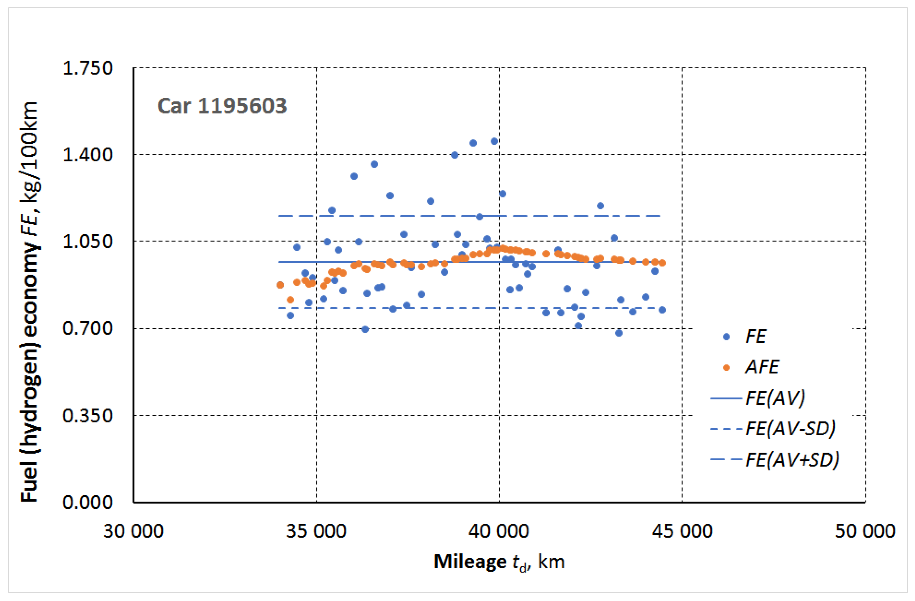
Figure 2.
Cumulative fuel (hydrogen) consumption in analyzed mileage of H2EV (No. 1195603).
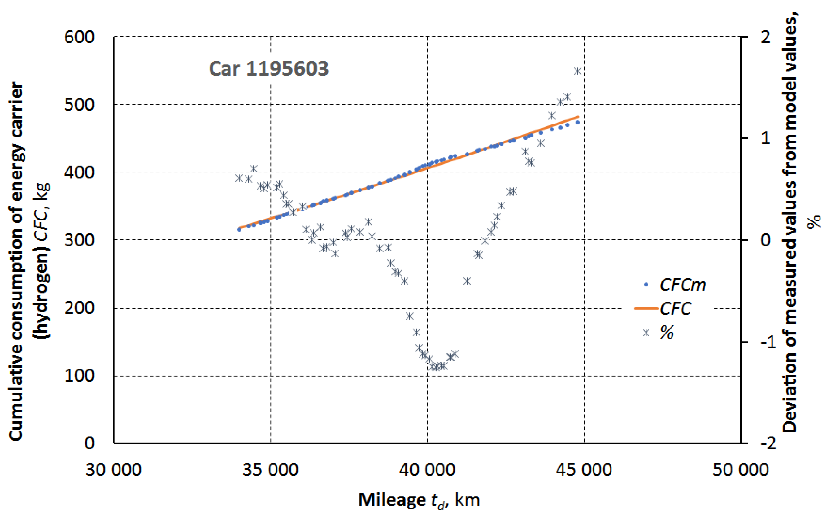
Figure 3.
Cumulative fuel consumption from beginning ap to 300,000km mileage of operation of the H2EV (No. 1195603).
Figure 3.
Cumulative fuel consumption from beginning ap to 300,000km mileage of operation of the H2EV (No. 1195603).
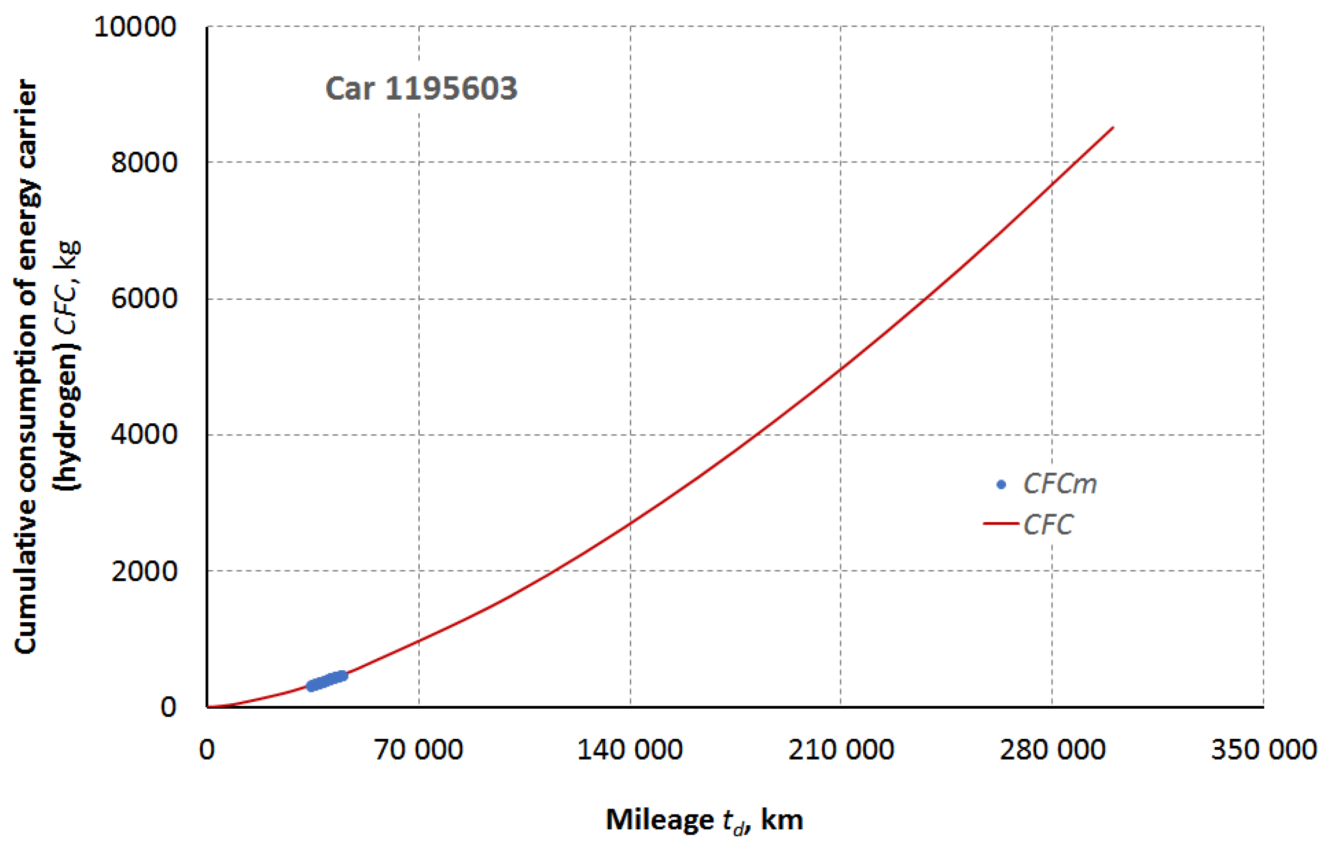
Figure 4.
Energy Foot Print the H2EV (No. 1195603).
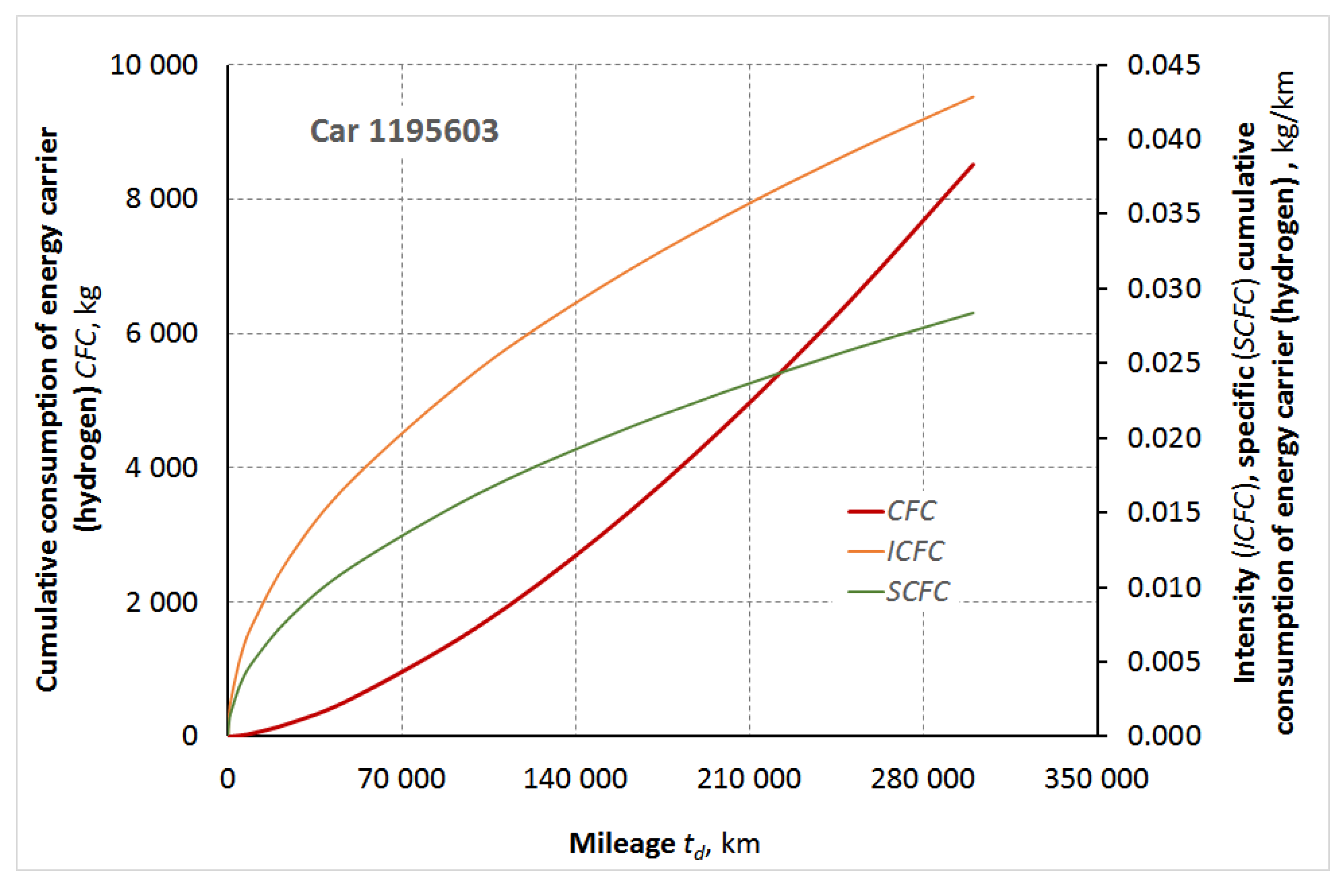
Figure 5.
Measured cumulative fuel consumption CFCm and the one determined CFC using model (3) with coefficients c and a as well as the predicted fuel consumption for 300,000 kilometers of each of the analyzed ICEVs.
Figure 5.
Measured cumulative fuel consumption CFCm and the one determined CFC using model (3) with coefficients c and a as well as the predicted fuel consumption for 300,000 kilometers of each of the analyzed ICEVs.
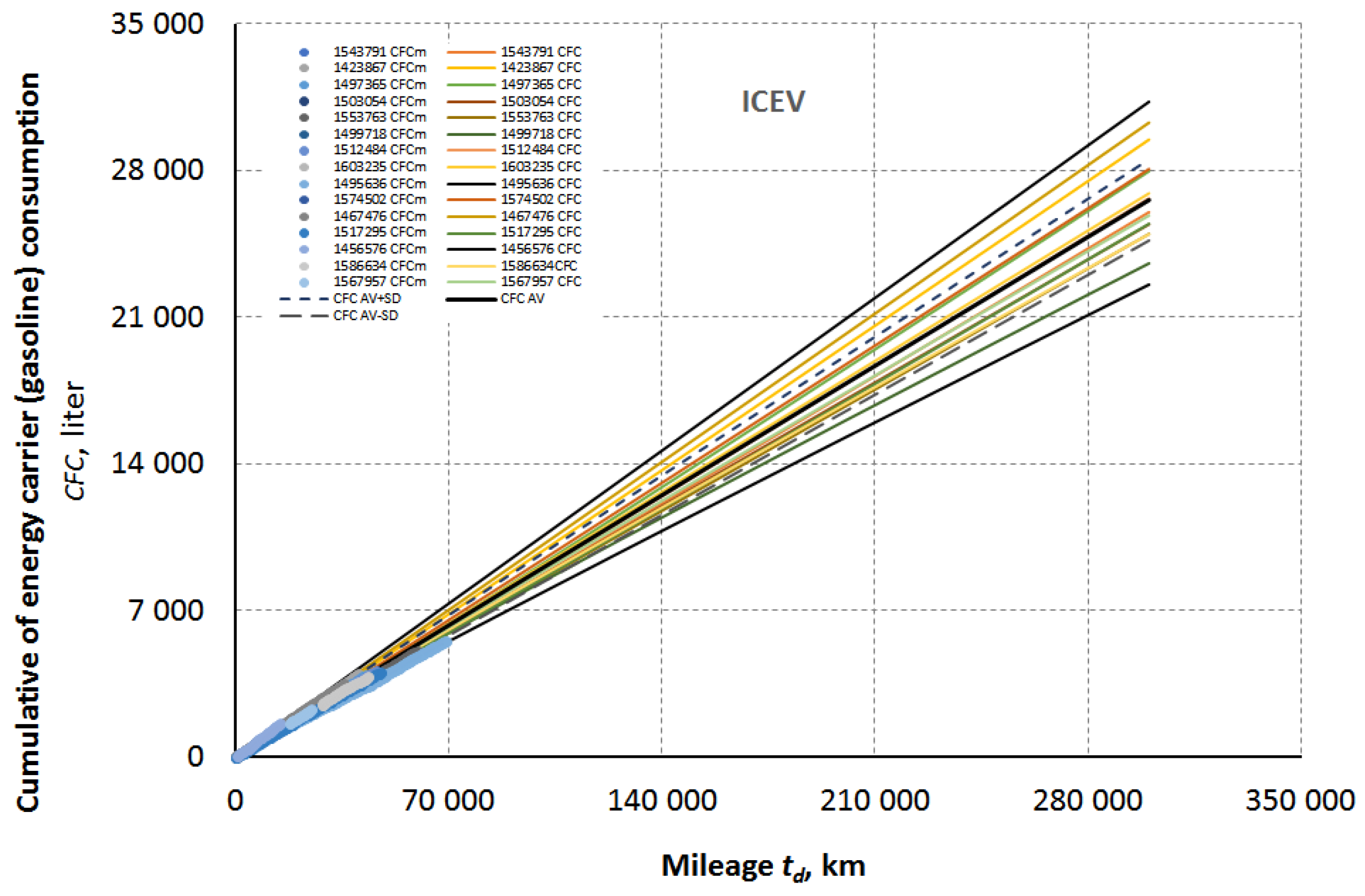
Figure 6.
Measured cumulative fuel consumption (CFCm) and the one determined CFC using model (3) with coefficients c and a as well as the predicted fuel consumption for 300,000 kilometers of each of the analyzed HEVs.
Figure 6.
Measured cumulative fuel consumption (CFCm) and the one determined CFC using model (3) with coefficients c and a as well as the predicted fuel consumption for 300,000 kilometers of each of the analyzed HEVs.
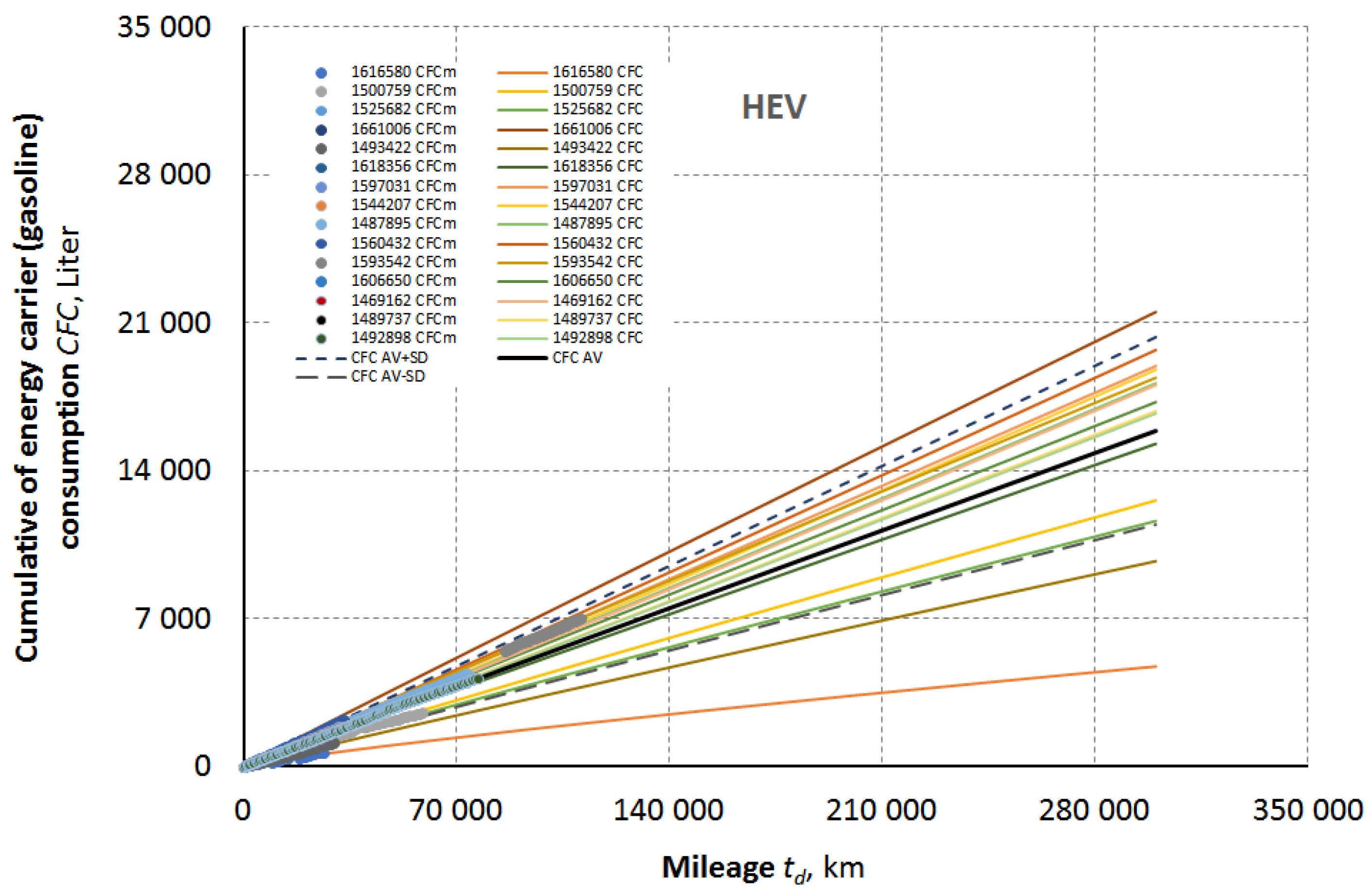
Figure 7.
Cumulative electricity consumption of the analyzed BEV’s.
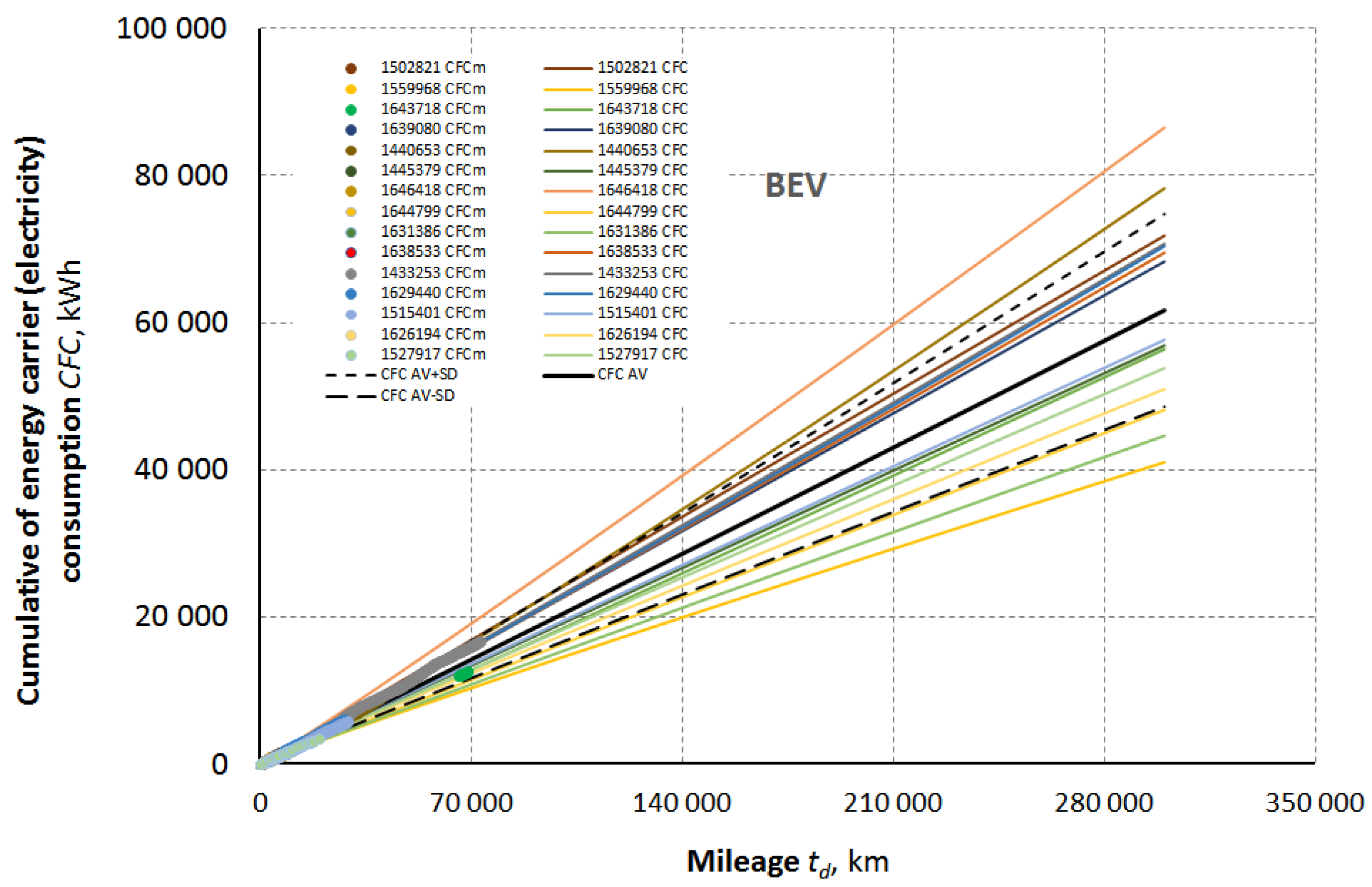
Figure 8.
Cumulative hydrogen consumption of the analyzed H2EV’s.
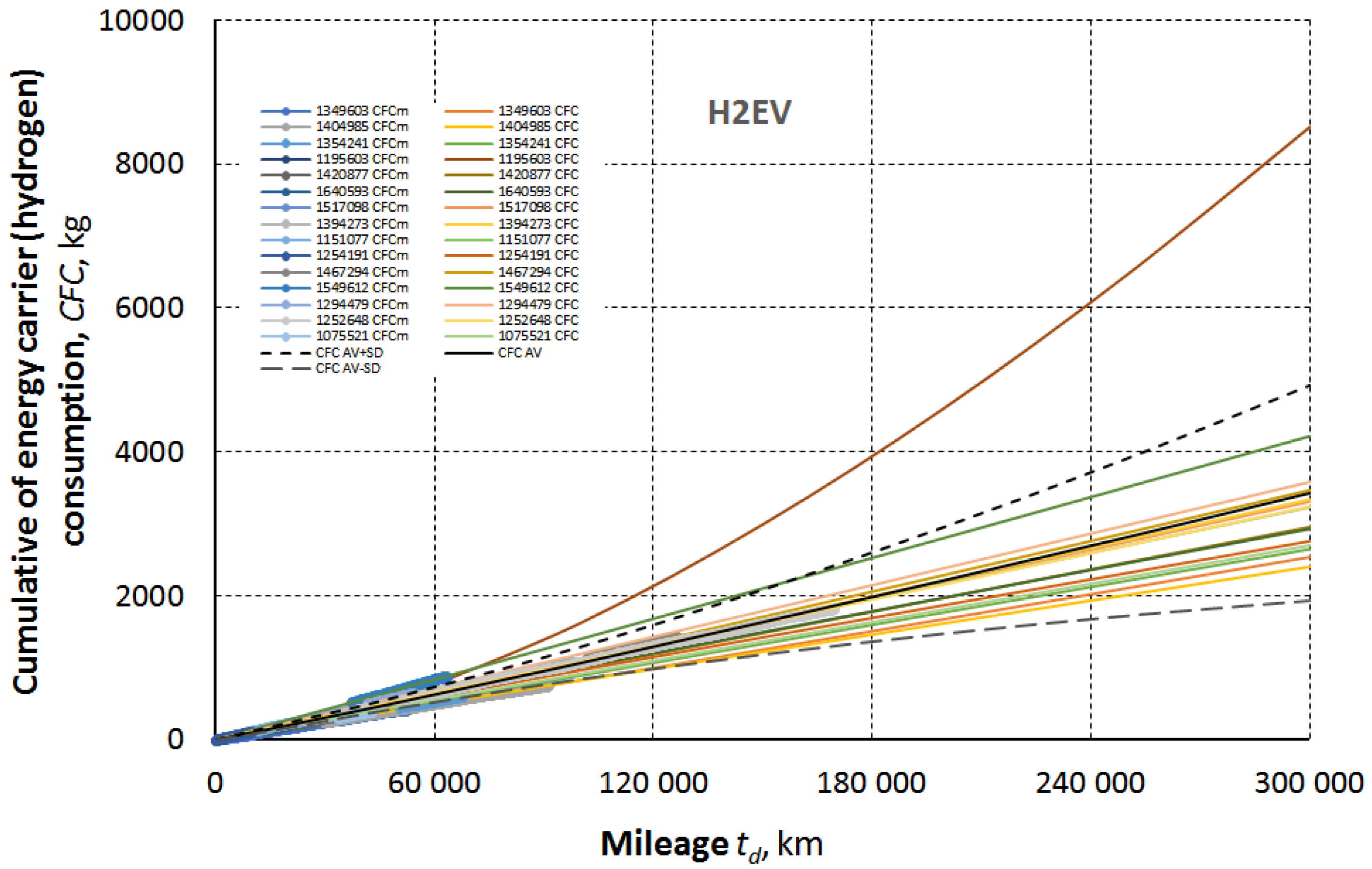
Figure 9.
Average energy carriers demand for driving the analyzed car from fleet cars types.
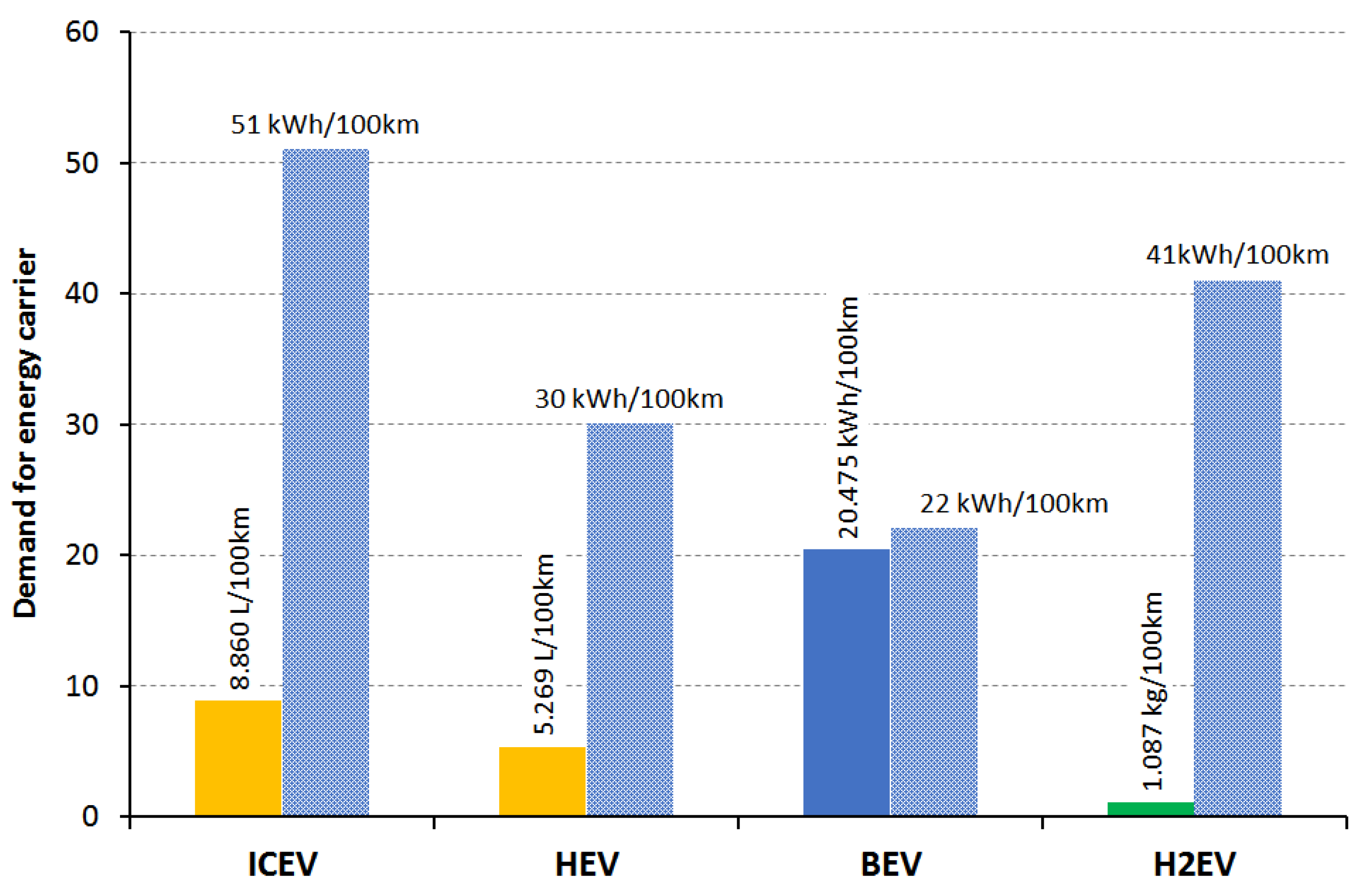

Table 1.
Hydrogen consumption operating data during long-term operation of H2EV no. 1195603 [20].
Table 1.
Hydrogen consumption operating data during long-term operation of H2EV no. 1195603 [20].
| No. | Datum | Tachostand [km] | Distanz [km] | Menge [kg] | FE [kg/100km] | AFE [kg/100km] | FE(AV) [kg/100km] | FE(AV-SD) [kg/100km] | FE(AV+SD) [kg/100km] | CFCm [kg] | CFC [kg] | % |
| 1 | 2021-08-26 | 44,797 | 563 | 4.38 | 0.778 | 0.968 | 0.968 | 0.784 | 1.153 | 474.43 | 482.451 | 1.66 |
| 2 | 2021-08-23 | 44,447 | 330.7 | 3.08 | 0.931 | 0.971 | 0.968 | 0.784 | 1.153 | 470.05 | 476.772 | 1.41 |
| 63 | 2020-08-22 | 34,454 | 274.1 | 2.07 | 0.755 | 0.816 | 0.968 | 0.784 | 1.153 | 322.31 | 324.599 | 0.70 |
| 64 | 2020-08-21 | 34,284 | 466.1 | 4.09 | 0.877 | 0.877 | 0.968 | 0.784 | 1.153 | 320.24 | 322.185 | 0.60 |
| 65 | 2020-08-15 | 33995 | 2.29 | 316.15 | 318.094 | 0.61 |
Where: Datum – Date of refueling; Tachostand – Vehicle odometer reading; Distanze – Distance traveled; Menge – Amount of fuel refueled. Full data (from row no. 1 to 65 of the table above) can be found at spritmonitor.de (or by authors).
Table 2.
Statistics of the fuel economy (FE) the H2EV no. 1195603.
| Mean [kg] | 0.968216 |
| Standard error [kg] | 0.023081 |
| Median [kg] | 0.939777 |
| Standard deviation [kg] | 0.184648 |
| Sample variance [kg] | 0.034095 |
| Kurtosis | 0.421764 |
| Skewness | 0.901152 |
| Range | 0.771085 |
| Minimum [kg] | 0.684353 |
| Maximum [kg] | 1.455437 |
| Sum [kg] | 61.965854 |
| Number | 64 |
| Confidence level (95.0%) [kg] | 0.046124 |
Table 3.
Statistics of model (3).
| Coefficients of Model (3) | |
| Coefficient c | 0.000046 |
| Coefficient a | 0.509577 |
| Statistics of Model (3) | |
| Multiple R | 0.998031 |
| R squared | 0.996066 |
| Fitted R squared | 0.996004 |
| Standard error | 0.007306 |
| Observations | 65 |
Table 4.
Information data of operation of ICEV’s.
| ICEV | Date b | Date e | Cer No | Mileage b [km] | Mileage e [km] | Trip distance [km] | Refueling | Highway [%] | City [%] | Country road [%] | Coefficient c | Coefficient a | R squared |
| 1 | 2024-08-23 | 2025-10-15 | 1567957 | 17 800 | 24 747 | 6 947 | 17 | 34 | 33 | 33 | 1.078045 | -0.992457 | 0.999115 |
| 2 | 2024-11-07 | 2025-10-17 | 1586634 | 28 315 | 43 313 | 14 998 | 31 | 37 | 27 | 36 | 0.120721 | -0.029543 | 0.997458 |
| 3 | 2023-06-20 | 2025-10-08 | 1456576 | 6 | 14 446 | 14 440 | 27 | 34 | 33 | 33 | 0.107580 | -0.002509 | 0.999093 |
| 4 | 2024-02-05 | 2025-09-16 | 1517295 | 9 | 47 460 | 47 451 | 85 | 33 | 34 | 33 | 0.083299 | 0.001438 | 0.999434 |
| 5 | 2023-08-07 | 2025-10-01 | 1467476 | 66 | 35 398 | 35 332 | 55 | 33 | 34 | 33 | 0.095383 | 0.004474 | 0.999820 |
| 6 | 2024-08-19 | 2025-09-13 | 1574502 | 15 | 21 423 | 21 408 | 63 | 32 | 34 | 34 | 0.092488 | 0.000889 | 0.998985 |
| 7 | 2023-11-12 | 2025-04-17 | 1495636 | 238 | 69 118 | 68 880 | 181 | 34 | 33 | 33 | 0.114243 | -0.033214 | 0.999001 |
| 8 | 2025-01-28 | 2025-10-15 | 1603235 | 290 | 20 609 | 20 319 | 46 | 59 | 3 | 38 | 0.102116 | -0.010304 | 0.999764 |
| 9 | 2024-11-26 | 2025-09-30 | 1512484 | 20 571 | 46 213 | 25 642 | 63 | 44 | 33 | 23 | 0.089105 | -0.000212 | 0.999771 |
| 10 | 2023-11-18 | 2024-08-30 | 1499718 | 27 732 | 39 090 | 11 358 | 19 | 34 | 33 | 33 | 0.149812 | -0.051221 | 0.999876 |
| 11 | 2024-06-27 | 2025-10-12 | 1553763 | 81 | 25 402 | 25 321 | 41 | 49 | 0 | 51 | 0.095295 | -0.010754 | 0.999906 |
| 12 | 2023-12-22 | 2025-10-05 | 1503054 | 81 | 25 402 | 25 321 | 41 | 36 | 28 | 36 | 0.098808 | -0.012178 | 0.999774 |
| 13 | 2023-11-09 | 2025-09-30 | 1497365 | 15 | 42 296 | 42 281 | 94 | 34 | 33 | 33 | 0.075207 | 0.016992 | 0.999069 |
| 14 | 2023-02-28 | 2025-09-24 | 1423867 | 25 | 40 344 | 40 319 | 79 | 13 | 34 | 53 | 0.091216 | 0.005854 | 0.999769 |
| 15 | 2023-09-08 | 2025-09-30 | 1543791 | 15 | 35 839 | 35 824 | 75 | 35 | 30 | 35 | 0.082744 | 0.003680 | 0.999912 |
Date b – should be understood as the start date of operational data recording [20]. Date e – should be understood as the end date of operational data recording [20]. Mileage b – should be understood as the vehicle’s mileage until the start of operating data recording [20]. Mileage e – should be understood as the vehicle’s mileage until the end of operating data recording [20]. Trip distance – should be understood as the difference of the Mileage e minus Mileage b. Refueling – should be understood as the number of refueling in a Trip distance. Highway – should be understood as the percentage of trips on motorways. City– should be understood as the percentage of city trips. Country road – should be understood as the percentage of trips on country road. Coefficient c – should be understood as the coefficient c in the equation (3). Coefficient a – should be understood as the statistical adequacy coefficient of the model (3) to the measurement data of cumulative fuel (energy) consumption.
Table 5.
Information data of operation of HEV’s.
| HEV | Date b | Date e | Cer No | Mileage b [km] | Mileage e [km] | Trip distance [km] | Refueling | Highway [%] | City [%] | Country road [%] | Coefficient c | Coefficient a | R squared |
| 1 | 2023-12-04 | 2025-10-18 | 1492898 | 17 800 | 76 811 | 59 011 | 127 | 49 | 18 | 33 | 1.011033 | -0.998930 | 0.999857 |
| 2 | 2023-10-18 | 2025-10-18 | 1489737 | 10 | 47 072 | 47 062 | 65 | 39 | 21 | 40 | 0.054417 | 0.002391 | 0.999811 |
| 3 | 2023-08-20 | 2025-10-19 | 1469162 | 6 | 32 150 | 32 144 | 48 | 34 | 33 | 33 | 0.054970 | 0.007177 | 0.999777 |
| 4 | 2025-02-15 | 2025-10-18 | 1606650 | 210 | 15 293 | 15 083 | 24 | 33 | 34 | 33 | 0.068781 | -0.014195 | 0.999673 |
| 5 | 2024-12-17 | 2025-10-23 | 1593542 | 85 810 | 149 239 | 63 429 | 127 | 33 | 34 | 33 | 0.090661 | -0.030971 | 0.999487 |
| 6 | 2024-07-22 | 2025-10-16 | 1560432 | 44 | 83 693 | 83 649 | 61 | 45 | 23 | 32 | 0.064151 | 0.001914 | 0.997837 |
| 7 | 2023-09-19 | 2025-10-18 | 1487895 | 10 | 73 516 | 73 506 | 129 | 36 | 28 | 36 | 0.059888 | 0.000764 | 0.999889 |
| 8 | 2024-07-05 | 2025-10-01 | 1544207 | 15 073 | 50 863 | 35 790 | 56 | 35 | 35 | 30 | 0.050585 | 0.016910 | 0.999870 |
| 9 | 2024-12-13 | 2025-10-11 | 1597031 | 10 | 19 885 | 19 875 | 36 | 50 | 50 | 0 | 0.066598 | -0.004171 | 0.999490 |
| 10 | 2024-01-17 | 2025-10-07 | 1618356 | 84 | 39 090 | 39 006 | 9 | 18 | 41 | 41 | 0.060356 | -0.013476 | 0.993225 |
| 11 | 2023-11-16 | 2025-09-07 | 1493422 | 483 | 30 203 | 29 720 | 41 | 0 | 53 | 47 | 0.056476 | -0.044071 | 0.993625 |
| 12 | 2025-08-10 | 2025-10-20 | 1661006 | 579 | 4 921 | 4 342 | 8 | 36 | 28 | 36 | 0.088051 | -0.016256 | 0.998309 |
| 13 | 2024-03-13 | 2025-08-30 | 1525682 | 299 | 42 296 | 41 997 | 23 | 33 | 33 | 34 | 0.075128 | -0.052507 | 0.995021 |
| 14 | 2023-12-06 | 2025-10-20 | 1500759 | 20 284 | 58 790 | 38 506 | 48 | 13 | 34 | 53 | 0.073913 | -0.044852 | 0.988640 |
| 15 | 2025-03-21 | 2025-10-21 | 1616580 | 1 283 | 26 279 | 24 996 | 18 | 38 | 31 | 31 | 0.100118 | -0.146478 | 0.980178 |
Table 6.
Information of operation data of analyzed BEV’s.
| BEV | Date b | Date e | Cer No | Mileage b [km] | Mileage e [km] | Trip distance [km] | Refueling | Highway [%] | City [%] | Country road [%] | Coefficient c | Coefficient a | R squared |
| 1 | 2024-03-18 | 2025-09-30 | 1527917 | 5 | 19 610 | 19 605 | 20 | 33 | 34 | 33 | 1.100572 | -0.989187 | 0.997848 |
| 2 | 2025-04-11 | 2025-10-15 | 1626194 | 10 | 9 197 | 9 187 | 32 | 37 | 30 | 33 | 0.230775 | -0.024268 | 0.999266 |
| 3 | 2024-03-02 | 2025-09-23 | 1515401 | 10 | 29 011 | 29 001 | 222 | 14 | 42 | 44 | 0.208959 | -0.006604 | 0.998368 |
| 4 | 2023-05-31 | 2025-10-25 | 1629440 | 6 | 28 233 | 28 227 | 132 | 33 | 34 | 33 | 0.158061 | 0.031354 | 0.998749 |
| 5 | 2023-04-20 | 2025-10-25 | 1433253 | 3 | 72 868 | 72 865 | 270 | 38 | 36 | 26 | 0.177246 | 0.022622 | 0.998900 |
| 6 | 2025-05-27 | 2025-10-24 | 1638533 | 15 | 3 918 | 3 903 | 21 | 27 | 36 | 37 | 0.171498 | 0.023874 | 0.990349 |
| 7 | 2025-05-10 | 2025-10-23 | 1631386 | 10 | 8 937 | 8 927 | 49 | 36 | 31 | 33 | 0.205619 | -0.025650 | 0.997791 |
| 8 | 2025-06-10 | 2025-10-16 | 1644799 | 390 | 10 564 | 10 174 | 16 | 17 | 42 | 41 | 0.186062 | -0.011719 | 0.999538 |
| 9 | 2025-07-04 | 2025-10-19 | 1646418 | 18 | 4 043 | 4 025 | 33 | 32 | 34 | 34 | 0.174579 | 0.039807 | 0.985246 |
| 10 | 2023-05-04 | 2024-05-03 | 1445379 | 84 | 39 090 | 39 006 | 63 | 16 | 42 | 42 | 0.200784 | -0.004521 | 0.988255 |
| 11 | 2023-04-14 | 2025-04-03 | 1440653 | 10 | 40 074 | 40 064 | 188 | 37 | 26 | 37 | 0.106756 | 0.070860 | 0.987708 |
| 12 | 2025-08-10 | 2025-10-20 | 1639080 | 122 | 5 869 | 5 747 | 37 | 33 | 33 | 34 | 0.202597 | 0.009269 | 0.996893 |
| 13 | 2025-06-19 | 2025-10-16 | 1643718 | 65 745 | 68 908 | 3 163 | 17 | 33 | 33 | 34 | 0.145314 | 0.020425 | 0.999139 |
| 14 | 2024-12-27 | 2025-10-25 | 1559968 | 173 | 8 933 | 8 760 | 30 | 41 | 44 | 15 | 0.262720 | -0.051739 | 0.995479 |
| 15 | 2023-12-21 | 2024-05-29 | 1502821 | 144 | 6 895 | 6 751 | 50 | 19 | 38 | 43 | 0.248051 | -0.002792 | 0.993011 |
Table 7.
Information of operation data of analyzed H2EV’s.
| H2EV | Date b | Date e | Cer No | Mileage b [km] | Mileage e [km] | Trip distance [km] | Refueling | Highway [%] | City [%] | Country road [%] | Coefficient c | Coefficient a | R squared |
| 1 | 2025-04-07 | 2025-10-19 | 1666344 | 33 584 | 42 553 | 8 969 | 27 | 33 | 34 | 33 | 0.011272 | -0.017869 | 0.998218 |
| 2 | 2021-04-29 | 2024-09-06 | 1252648 | 38 208 | 166 493 | 128 285 | 279 | 0 | 100 | 0 | 0.011226 | -0.003039 | 0.999695 |
| 3 | 2021-10-15 | 2024-10-23 | 1294479 | 41 574 | 54 340 | 12 766 | 39 | 51 | 49 | 0 | 0.011769 | 0.001151 | 0.999797 |
| 4 | 2024-06-07 | 2025-08-13 | 1549612 | 37 362 | 63 466 | 26 104 | 97 | 72 | 4 | 24 | 0.013390 | 0.003875 | 0.999743 |
| 5 | 2023-07-19 | 2025-10-27 | 1467294 | 102 098 | 126 531 | 24 433 | 89 | 24 | 0 | 76 | 0.008772 | 0.021917 | 0.999163 |
| 6 | 2021-07-24 | 2022-05-20 | 1254191 | 20 | 9 952 | 9 932 | 40 | 35 | 32 | 33 | 0.016115 | -0.044467 | 0.993667 |
| 7 | 2019-10-24 | 2025-10-08 | 1151077 | 114 | 98 774 | 98 660 | 377 | 38 | 30 | 32 | 0.014005 | -0.020798 | 0.999260 |
| 8 | 2022-05-03 | 2024-06-21 | 1394273 | 26 359 | 61 110 | 34 751 | 120 | 38 | 27 | 35 | 0.009529 | 0.012368 | 0.999581 |
| 9 | 2025-07-04 | 2025-10-19 | 1517098 | 18 | 4 043 | 4 025 | 12 | 27 | 34 | 39 | 0.009613 | 0.010938 | 0.998481 |
| 10 | 2025-05-23 | 2025-10-26 | 1640593 | 14 651 | 20 206 | 5 555 | 16 | 50 | 47 | 3 | 0.014181 | -0.029572 | 0.998546 |
| 11 | 2023-01-21 | 2025-01-01 | 1420877 | 13 971 | 39 695 | 25 724 | 65 | 30 | 28 | 42 | 0.010460 | -0.004716 | 0.998654 |
| 12 | 2020-08-15 | 2021-08-26 | 1195603 | 33 995 | 44 797 | 10 802 | 65 | 16 | 24 | 60 | 0.000046 | 0.509577 | 0.996066 |
| 13 | 2022-05-03 | 2023-01-21 | 1354241 | 505 000 | 67 703 | -437 297 | 45 | 51 | 37 | 12 | 0.009850 | -0.008676 | 0.999241 |
| 14 | 2022-11-16 | 2025-04-04 | 1404985 | 29 504 | 91 226 | 61 722 | 166 | 39 | 34 | 27 | 0.010930 | -0.024585 | 0.999514 |
| 15 | 2022-04-22 | 2025-10-26 | 1349603 | 24 | 52 867 | 52 843 | 111 | 53 | 44 | 3 | 0.006601 | 0.019707 | 0.999361 |
Table 8.
CFC Mean, CFC Standard Deviation and 100CFC for each vehicles group.
| ICEV | ICEV | ICEV | HEV | HEV | HEV | BEV | BEV | BEV | H2EV | H2EV | H2EV | |
| Mileage td [km] | CFC Mean [L] | CFC Standard deviation [L] | 100SCFC [L/100km] | CFC Mean [L] | CFC Standard deviation [L] | 100CFC [L/100km] | CFC Mean [kWh] | CFC Standard deviation [kWh] | 100SCFC [kWh/ 100km] |
CFC Mean [kg] | CFC Standard deviation [kg] | 100SCFC [kg/100km] |
| 10 | 0,978 | 0,137 | 9,783 | 0,639 | 0,104 | 6,389 | 1,930 | 0,301 | 19,300 | 0,102 | 0,035 | 1,015 |
| 100 | 9,545 | 0,968 | 9,545 | 6,062 | 0,947 | 6,062 | 19,426 | 2,306 | 19,426 | 1,000 | 0,319 | 1,000 |
| 500 | 46,956 | 3,751 | 9,391 | 29,341 | 5,089 | 5,868 | 97,828 | 10,664 | 19,566 | 4,968 | 1,478 | 0,994 |
| 1 000 | 93,281 | 6,786 | 9,328 | 57,922 | 10,636 | 5,792 | 196,386 | 21,685 | 19,639 | 9,923 | 2,824 | 0,992 |
| 5 000 | 459,428 | 29,291 | 9,189 | 281,527 | 59,122 | 5,631 | 991,986 | 125,074 | 19,840 | 49,810 | 11,842 | 0,996 |
| 10 000 | 913,131 | 58,237 | 9,131 | 556,674 | 123,504 | 5,567 | 1 994,022 | 273,437 | 19,940 | 100,244 | 20,847 | 1,002 |
| 25 000 | 2 264,537 | 152,524 | 9,058 | 1 371,804 | 325,917 | 5,487 | 5 021,571 | 776,144 | 20,086 | 254,426 | 42,048 | 1,018 |
| 50 000 | 4 502,331 | 325,589 | 9,005 | 2 715,215 | 677,159 | 5,430 | 10 103,488 | 1 711,529 | 20,207 | 518,494 | 80,864 | 1,037 |
| 100 000 | 8 952,736 | 705,102 | 8,953 | 5 376,345 | 1 403,603 | 5,376 | 20 336,663 | 3 769,114 | 20,337 | 1 066,013 | 223,598 | 1,066 |
| 150 000 | 13 384,602 | 1 111,667 | 8,923 | 8 018,836 | 2 147,635 | 5,346 | 30 625,159 | 5 974,357 | 20,417 | 1 633,592 | 449,371 | 1,089 |
| 200 000 | 17 804,661 | 1 536,441 | 8,902 | 10 649,580 | 2 902,847 | 5,325 | 40 951,084 | 8 278,616 | 20,476 | 2 217,660 | 742,550 | 1,109 |
| 250 000 | 22 216,052 | 1 974,998 | 8,886 | 13 271,763 | 3 666,254 | 5,309 | 51 305,604 | 10 658,026 | 20,522 | 2 816,097 | 1 093,555 | 1,126 |
| 300 000 | 26 620,606 | 2 424,660 | 8,874 | 15 887,227 | 4 436,121 | 5,296 | 61 683,379 | 13 098,236 | 20,561 | 3 427,451 | 1 496,110 | 1,142 |
Table 9.
The 100SCFC results for the 300,000 km mileage of the individual vehicle groups.
| ICEV | HEV | BEV | H2FCEV | ||
| Gasoline | Gasoline | Electricity | Hydrogen | ||
| [L/100km] | [L/100km] | [kWh/100km] | [kg/100km] | ||
| 1 | 100SCFC(300000) | 8.860 | 5.269 | 20.475 | 1.087 |
Table 10.
Conversion factors used in this study for energy assesing.
| Parameter | Symbol | Value | Source | |
| Gasoline energy density (LHV) |  |
8.8 kWh/L (31.7 MJ/L) | JEC, 2020 | |
| Electricity conversion | — | 1 kWh = 3.6 MJ | Standard | |
| Refinery electricity demand |  |
1.2 kWh/L gasoline | IEA, 2023 | |
| Hydrogen energy density |  |
33.3 kWh/kg (120 MJ/kg) | JRC, 2020 | |
| Electrolysis efficiency |  |
70% (LHV basis) | IEA, 2023 | |
| Compression + dispensing losses |  |
90% | JEC, 2020 | |
| Grid-to-battery efficiency (BEV) |  |
90–92% | EEA, 2024 | |
| Battery-to-wheel efficiency (BEV) |  |
90–95% | IEA, 2023 | |
Disclaimer/Publisher’s Note: The statements, opinions and data contained in all publications are solely those of the individual author(s) and contributor(s) and not of MDPI and/or the editor(s). MDPI and/or the editor(s) disclaim responsibility for any injury to people or property resulting from any ideas, methods, instructions or products referred to in the content. |
© 2025 by the authors. Licensee MDPI, Basel, Switzerland. This article is an open access article distributed under the terms and conditions of the Creative Commons Attribution (CC BY) license (http://creativecommons.org/licenses/by/4.0/).
Copyright: This open access article is published under a Creative Commons CC BY 4.0 license, which permit the free download, distribution, and reuse, provided that the author and preprint are cited in any reuse.


