Submitted:
11 December 2025
Posted:
12 December 2025
You are already at the latest version
Abstract
Recently, Figueroa et al. demonstrated that steady streaming can be generated by the oscillatory motion of a floating magnet driven by electromagnetic forcing in a shallow electrolytic layer. They also found that the rotation direction of the resulting steady vortices is opposite to that of classical streaming flows. In this work, we present a theoretical and experimental investigation of the fluid–structure interaction between a freely moving wall and an oscillatory flow. Our objective is to elucidate the coupling mechanism between the fluid and the oscillating body that gives rise to reverse streaming and to apply this analysis to the case of a freely moving wavy wall. The flow is analyzed theoretically and an analytical solution is obtained using a perturbation method. Experimental results based on Particle Image Velocimetry are also presented, where an oscillatory flow generated by an electromagnetic force in an electrolyte layer drives a wavy wall floating on the surface. The results confirm the occurrence of reverse streaming and demonstrate that the flow dynamics depend on the density ratio between the freely moving solid and the fluid. The analytical solution qualitatively captures the behavior observed in the experiments.
Keywords:
steady streaming
; oscillatory flow
; vortical structures
; boundary layer
; wavy wall
; perturbation method
; particle image velocimetry
1. Introduction
A wide range of natural phenomena and engineering applications feature oscillatory flows confined by rigid or deformable boundaries. In such systems, the presence of dissipation together with nonlinear convective effects can produce a net transport of mass, momentum, and heat, even when the flow has zero mean. Examples of this kind of flows occur in physiological [1,2] and oceanographic phenomena [3,4], as well as in applications aimed at enhancing heat transfer [5,6].
The classical solution to Stokes’ second problem [7], which describes the motion generated when a flat plate oscillates harmonically in its own plane within a still viscous fluid, exemplifies the fundamental behavior of oscillatory viscous flow near a solid wall. In Stokes’ linear solution, wall oscillations produce an oscillatory flow of the same frequency, whose amplitude decays exponentially away from the wall. When nonlinear convective effects occur, such as those introduced by wall curvature, mass conservation gives rise to a transverse velocity component. Consequently, a secondary flow develops, comprising an oscillatory component at twice the driving frequency and a steady part, called steady streaming [8,9]. The latter is the generation of a steady recirculating motion that arises from a primary zero-mean oscillatory flow induced by vibrating boundaries or a pulsating pressure field. This phenomenon is a second-order effect produced by nonlinear Reynolds stresses within the unsteady boundary layer, which make the time-averaged oscillatory motion nonzero. Due to viscous effects, the resulting steady flow extends beyond the boundary layer, a defining feature of steady streaming [10].
Among the seminal works on steady streaming are the classic contributions of Rayleigh [11] and Schlichting [12,13]. Early studies of this phenomenon focused mainly on the oscillatory motion of cylinders [10,14,15] or spheres [16,17,18] immersed in a quiescent viscous fluid. More recently, interest in steady streaming has resurged due to its potential for a variety of microfluidic applications, including enhanced mixing [19,20] and manipulation of suspended particles [21,22]. Streaming flows induced by microbubbles have also been used for particle sorting [23]. In many of these applications, acoustic techniques play a central role in generating the streaming flow [24]. Moreover, the possibility of using streaming in biological processes or for bioengineering purposes has recently been proposed. For instance, fluid oscillations around a fixed cylinder in a microchannel can generate streaming eddies that can trap and levitate cells without direct contact [25]. Streaming flows have also been proven to be valuable for a wide range of tasks, including microparticle transport and manipulation, regulation of particle flocculation [26] and drug delivery [27,28].
Streaming generation, whether at the macroscopic or microscopic scale, has been mostly achieved using mechanical or acoustic transducers that induce oscillations of solid bodies or bubbles immersed in the fluid, or by employing pumps that drive the flow, for example, in microchannels. Electromagnetic approaches for generating streaming have also been investigated numerically, considering a quiescent layer of liquid metal disturbed by an external oscillating dipole magnet [29,30]. More recently, an alternative configuration involving a floating free moving magnet on an electrolyte layer subjected to an alternating electric current demonstrated, both experimentally and theoretically, the feasibility of inducing streaming [31]. Moreover, an unexpected effect was found, namely that the rotating sense of streaming vortices reverses with respect to the classical case of an oscillating cylinder. The coupling between the fluid and the free-moving body has been identified as the cause of reverse streaming.
The present work extends previous investigations by performing a theoretical and experimental analysis of the boundary-layer flow induced by a freely moving wavy wall in a viscous fluid. Considering boundary waviness provides an effective model for representing the perturbations introduced by wall roughness, which are particularly important at microscales [32,33,34]. First, assuming that the thickness of the Stokes layer is much smaller than the wavelength of the wall, the axial viscous diffusion terms can be neglected, producing a formulation of the boundary-layer of the problem [35,36], in which the boundary condition of the free-moving wall is incorporated. Next, by applying a suitable coordinate transformation, an analytical solution is obtained using a perturbation method, under the assumption that the oscillation amplitude of the fluid is small relative to the wall wavelength, thus preventing boundary-layer separation [10]. The second-order solution captures the steady streaming flow and confirms that its direction can be reversed by varying the density ratio between the fluid and the wall. Furthermore, theoretical predictions are qualitatively validated through experiments in which a freely moving wavy wall floating on an electrolyte layer is set into oscillatory motion by an electromagnetic force, leading to the formation of steady streaming vortices.
2. Formulation of the Problem
We analyze the oscillatory motion of an incompressible Newtonian liquid limited by a free-moving infinite wavy wall which is described by the equation
where A and L are the amplitude and wavelength of the wall, while x is the stream-wise coordinate (see Figure 1). The flow is driven by a harmonic pressure gradient applied in the x-direction so that far from the wavy wall, the fluid performs an oscillatory motion about a zero mean whose axial velocity can be expressed as , where is the velocity amplitude and is the angular frequency of oscillation. The governing equations of motion of an incompressible Newtonian fluid are the continuity equation,
and the momentum balance equation,
where is the velocity field, p is the pressure field, is the kinematic viscosity and is the mass density of the fluid. In two-dimensional flow, the continuity and momentum equations can be expressed as
where u and v are the velocity components in the streamwise and transverse directions, respectively. We now introduce the following non-dimensional variables
where is the thickness of the Stokes layer, . The dimensionless expressions of the continuity and momentum equations are
where , while, for simplicity, the over line in u, v and p has been removed. The parameter can be interpreted as the ratio of the displacement amplitude of the fluid, , to the wavelength of the wall, L. To ensure the absence of boundary-layer separation, we will assume that the small amplitude of the oscillation condition holds, that is, [10]. Moreover, we assume that the thickness of the Stokes layer is much smaller than the wavelength of the wavy wall, that is, , therefore, the axial viscous diffusion terms in equations (9) and (10) can be neglected, indicating that the transport of momentum by viscous diffusion is much stronger in the transversal than in the horizontal direction, so that
From equation (12), we observe that . Therefore, we end up with the following boundary layer problem
which must satisfy both the matching condition for the streamwise velocity with the outer flow outside the boundary layer and the interaction with the free-moving wavy solid wall. At the free-moving wavy wall, the fluid is required to satisfy the no-slip boundary condition. Therefore, the boundary conditions that equations (13) and (14) must satisfy are the following:
where is the dimensionless amplitude of the wall and and are the velocity components of the wall. If we use the coordinate transformation,
that consists of a change to a reference frame where the wall is flat, the boundary conditions can be simplified. Under this transformation,
In order to satisfy volumetric flow conservation, the waviness of the wall must be taken into account. At the crest, the boundary layer removes a fluid volume equal to , which corresponds to the flow deficit created by the boundary layer (see Figure 1). Because the flow is incompressible, the same deficit must appear in every transverse section, which yields the following balance equation
where is the velocity modified by the presence of the wavy wall. In dimensionless terms, we have the following
Expressed in the coordinate frame in which the wall is rendered flat, the nondimensional outer flow becomes
where denotes the real part of the quantity in the brackets. On the other hand, the momentum balance equation satisfied by the outer flow is
which represents the pressure gradient required to balance the inertia in the outer flow. Using transformation (17) and substituting outer-flow expression (22) to eliminate the pressure, equations (13) and (14) become
which must satisfy the boundary conditions
To solve the system of equations, we must provide an explicit expression for the velocity of the wall ), since it serves as a boundary condition that directly shapes the motion of the fluid near the wall. For this purpose, we apply Newton’s second law to the wall, which gives the balance between its inertia and the external forces acting on it. The dimensionless governing equation for the motion of the wall is
where is the force vector field and is a dimensionless parameter that represents the ratio of wall density to fluid density . If , in such a way that , the inertia of the wall dominates, which corresponds to a fixed wall problem where the wall acceleration is zero. In turn, when , implies that the inertia of the wall is negligible, similar to the case where there is no wall and the potential flow remains. For this study, the solid wall is free to move only in the horizontal direction, so , therefore, the horizontal component of the acceleration in equation (27) has to be balanced by the drag force on the wall in this direction. Hence, considering the boundary layer approximation, Newton’s second law for the solid wall takes the form
where the term in parentheses on the right-hand side of (28) is the contribution of pressure and shear stress to the drag force on the wall [37].
3. Perturbation Solution
Let us now assume that the velocity components, streamwise, u, and transversal, v, along with the pressure and the wall velocity, can be expressed as a perturbation expansion on the small parameter for arbitrary values of a, that is,
where subscripts 0 and 1 denote the first- and second order approximations, respectively.
3.1. First Order Approximation
If we substitute expressions (29) and (30) into (24) and equate the coefficients of powers of , we obtain
which must satisfy the boundary conditions
along with
where satisfies (22) with the boundary condition . This problem is the generalization of the Stokes’ second problem with a free moving wall [31]. We can look for the solution in the form
where is a constant that depends on the waviness of the wall and has to be determined. Introducing (37) into (33), we find the equation
which must satisfy and as . Here, , and the constant can be expressed as . The solution of (38) that satisfies the boundary conditions coupled with Newton’s second law for the wall (28) is
In order to determine , (37) and (39) are substituted in (36), along with obtained from the solution of equation (22). Once this is done, we find from (36)
where
In (40), and correspond to the contributions of pressure and shear stress to the drag force, respectively. Therefore, at first order, the velocity component in the streamwise direction is
or explicitly
Figure 2 shows the normalized axial velocity as a function of the transverse coordinate , for a fixed time () and different values. When , the system approaches the limit of a vanishingly light wall (i.e., the density of the wall tends to zero), and the normalized axial velocity matches the amplitude of the potential flow throughout the entire domain. As increases (), a phase lag emerges between the fluid response and the wall motion, and the velocity at the wall () becomes non-zero. For large values of (), the system approaches the fixed-wall limit, corresponding to a boundary condition of zero-velocity at the wall.
Figure 3 shows the axial velocity as a function of the transverse coordinate , at different times with and for two representative values of . The fixed-wall case (), is shown in Figure 3(a). In this situation, the wavy wall has a density much larger than that of the fluid, so its inertia dominates and the wall effectively remains stationary (zero velocity). Consequently, its inertia predominates, and the wall remains stationary (at zero velocity). This case corresponds to the modified Stokes’ second problem [31]. Furthermore, Figure 3(b) presents the freely moving light wall case (), where displays a nonzero value at at every instant, matching the instantaneous wall velocity.
3.2. Second Order Approximation
From equations (24), (29) and (30), the equation governing the second order approximation (()) is found to be
It is worth noting that the right-hand side of Equation (44) contains convective terms proportional to . Consequently, besides the oscillatory components at twice the fundamental frequency, the nonlinear terms also generate time-independent contributions responsible for the steady streaming flow. With these considerations, is expressed in the form
where the subscripts u and s refer to the unsteady and steady parts, respectively. The equations satisfied by and can be found by substituting (37), (43) and (45) in Equation (44). In fact, the steady part satisfies
where conjugate complex quantities are denoted by the over bar. As occurs in the classical steady streaming case [10,13], it is impossible to satisfy condition (48) at infinity if condition (47) is imposed on the wall. Therefore, condition (48) must be relaxed by enforcing to take a finite value as . The solution of Equation (46) that satisfies the relaxed boundary conditions is
Taking the limit when the wall density tends to infinity (), Equation (49) reduces to the corresponding expressions for the classical streaming case with a fixed wall [10,12,13]. Therefore, the second-order steady velocity components parallel and transverse to the wall can be expressed, respectively, as
where satisfies the boundary condition at . In the classical case with a fixed plate the steady tangential velocity, , at the edge of the boundary layer () yields Rayleigh’s law of streaming [10,13], namely,
This steady velocity is originated by the Reynolds stresses related to oscillatory viscous flow [10]. In the case of a moving wall, the classical Rayleigh law of streaming is modified as follows:
where
If we take the limit where the density of the wall tends to infinity (), equation (54) recovers the classical Rayleigh’s law of streaming for a fixed wall, i.e., . This behavior is illustrated in Figure 4 which shows , normalized with , as a function of for different values of the parameter . It can be observed that at the edge of the inner boundary layer (), the limit value of the normalized function increases from negative values ( -3/4 for ) to higher values as decreases. In fact, for the normalized value is approximately zero and becomes positive for , indicating a reversal in the direction of the steady axial velocity. The fact that the reversal occurs for small values of (), confirms that this effect is a direct consequence of the free-motion condition of the wall. It is important to note that the nonzero axial velocity at the edge of the boundary layer, given by Equation (50), reflects the penetration of the steady streaming flow—either normal or reversed, depending on the value of R—into the outer potential flow.
An illustrative way to show the appearance of reverse steady streaming is to plot the steady vorticity in the z-direction, , which in the present problem is given as
In Figure 5, the velocity field is superimposed on a background color map representing the vorticity field over one wall wavelength, obtained from Equation (55) for different values of , assuming a small wall amplitude (). Figure 5(a) illustrates the case , where two small counter rotating vortices are located near the wall, while an upper pair of vortices extends into the potential flow. As decreases to 2 and 1.5 (Figure 5(b) and (c)), the lower vortices increase in both size and intensity. Finally, when , Figure 5(d) shows only two elongated vortices with a reversed sense of rotation compared with the case, penetrating into the outer potential flow.
4. Experiments
We now experimentally investigate the steady streaming induced by the freely moving wavy wall. From an experimental standpoint, the simplest way to realize a freely moving wall driven by an oscillating fluid is to float the wall on a liquid layer. The experimental setup consists of a glass container (30 cm × 15 cm × 16 cm) partially filled with an electrolyte solution to a height of cm. A plastic wavy plate floats freely on the surface, while an oscillating Lorentz force drives the fluid motion, as shown in Figure 6. The working fluid is a weak electrolytic solution of sodium bicarbonate at 8.6% by weight. At room temperature (), the mass density, kinematic viscosity, and electrical conductivity of the electrolyte are Kg/, /s and S/m, respectively. A magnetic field is generated by a rectangular permanent magnet (8 cm × 5 cm × 0.5 cm) located beneath the container. The maximum magnetic field intensity, measured with a Tesla meter (F.W. Bell, model 048) at the magnet surface, is 0.5 T. An oscillatory electric current is applied between two parallel graphite electrodes using a Tektronix CFG250 function generator. The frequency and amplitude of the electric current are set to 300 mHz and 120 mA, respectively. Under these conditions, electrolysis remains negligible. The origin of the coordinate system is located at the geometric center of the container’s bottom wall. The plane lies within the vertical plane of the setup, with the y-axis oriented normal to the bottom wall, while the z-axis points in the perpendicular direction. The alternating electric current applied along the z-direction interacts with the magnetic field, whose main component lies in the y-direction, generating a Lorentz force that drives the fluid into oscillatory motion along the x-direction.
The wavy plate (7.8 cm × 4.8 cm × 2.0 cm) is made of 3D-printed ABS plastic and has a sinusoidal surface profile with amplitude 2 mm and wave length mm. The plate is polished and then coated with Fast Dry Acrylic Enamel to smooth the surface. The density of the floating plate, , is adjusted by placing small weights on its surface, increasing its effective density from 1020 to 5260 Kg/. As a result, the corresponding density ratio spans the range .
Velocity fields are obtained with particle image velocimetry (PIV) in the plane. Silver coated glass spheres (10 m in diameter) are illuminated with a green laser sheet for the PIV measurements. To minimize three-dimensional effects arising from the lateral boundaries in the z-direction of the wavy wall, the laser sheet is projected onto the mid-plane (). Consequently, the experiments are conducted under conditions that approximate two-dimensional flow behavior. The video recordings are captured using a Nikon D80 camera with an AF Micro-Nikkor 60 mm f/2.8 lens. After the transient state, the recorded images are analyzed using PIVLab [38]. The maximum amplitude of the experimental velocity was mm/s. Therefore, the corresponding Reynolds number, =15, indicates a laminar flow. In turn, the parameter is smaller than unity (), ensuring the absence of boundary layer separation [10]. In addition, the Stokes layer thickness m is much smaller than the wavelength L, yielding a ratio of . Finally, the dimensionless wall amplitude is .
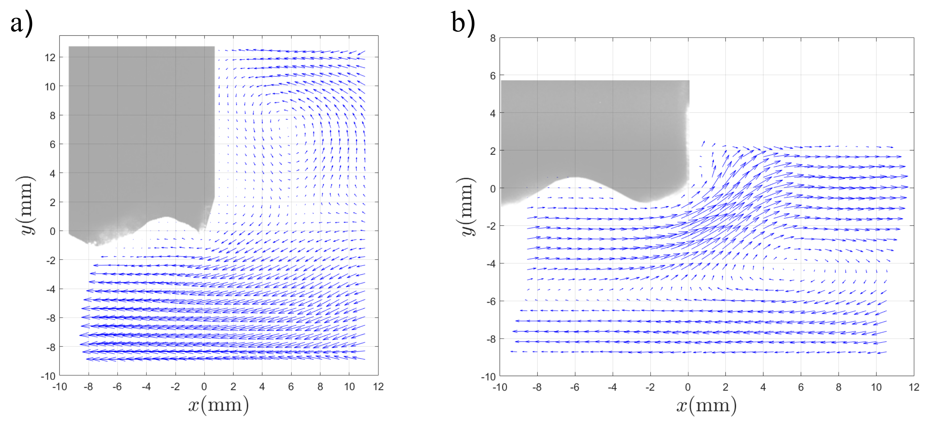
The PIV data are phase-averaged over one oscillation cycle to extract the steady streaming component. The resulting streaming velocity fields are presented in Figure 7. Because of the finite size of the wavy wall, vortex formation is most clearly observed near the edges of the plate, where the change in curvature is more pronounced. A large vortical structure with positive rotation is observed in the upper flow region for (see Figure 7a)). In addition, slight signs of a very small vortex located below the large vortex structure can be observed, a feature that qualitatively agrees with the theoretical prediction of the steady streaming flow shown in Figure 5a). Figure 7b) corresponds to the case where the plate sinks to a shallower depth due to its lower density. In this case, only a large vortex with positive rotation is observed in the lower region of the flow which coincides with the theoretical prediction of the reverse steady streaming in Figure 5d).
5. Discussion and Concluding Remarks
We have investigated, both theoretically and experimentally, the fluid–structure interaction between a freely moving wavy wall and an imposed oscillatory laminar flow. This configuration represents a generalization of the modified Stokes’ second problem with a free-moving wall [31]. The study focuses on the steady streaming flow generated by nonlinear Reynolds stresses within the boundary layer, which arise due to the wall’s curvature. In particular, the objective was to demonstrate that the direction of rotation of the streaming vortices reverses when the density ratio between the wall and the fluid becomes sufficiently small.
The theoretical model considers an infinite wavy wall subjected to a harmonically oscillating potential flow that generates a boundary-layer motion. Using a perturbation approach in which the dimensionless displacement amplitude of the fluid is treated as a small parameter, the boundary-layer equations are solved in conjunction with Newton’s second law for the wall, which balances the wall’s inertia with the drag force exerted by the fluid. The solution, expressed in terms of the density ratio between the wall and the fluid, exhibits a first-order oscillatory response with a phase lag between the wall motion and the fluid motion. When , the inertia of the wall dominates and the fixed-wall limit is recovered. In contrast, for , the drag force exceeds the inertial effects, and the phase lag between the two motions becomes pronounced. The second-order solution contains both a harmonic component oscillating at twice the original frequency and a steady streaming contribution. As in the classical case [10], the streaming flow does not vanish at the edge of the boundary layer but instead penetrates into the outer flow which leads to a modified Raylegh’s law of streaming. The results clearly show that as the density ratio decreases to , the direction of rotation of the steady vortices that extend into the outer flow is reversed, confirming that this reversal originates from the free motion of the wall.
The experimental setup consisted of a plastic wavy wall with adjustable density, floating on a layer of electrolyte driven by an oscillating Lorentz force. Velocity fields were measured with PIV and averaged over a complete oscillation period, revealing the steady streaming pattern. Experimental limitations prevent an exact reproduction of the theoretically studied problem, primarily because the finite size of the wavy wall introduces effects not accounted for in the theoretical model. Consequently, comparison between the experimental observations and theoretical predictions can only be qualitative, as the experimental setup does not fully satisfy the simplifying assumptions underlying the model. Furthermore, the limited resolution of the PIV system prevents visualization of the boundary-layer flow within the wall’s wavy regions, revealing only the larger flow structures that develop near the wall edges. Nevertheless, the main objective—experimental verification of the reversal of steady streaming by varying the density ratio between the wall and the fluid—was successfully achieved. In future experimental studies, adjusting the oscillation frequency—and thus the boundary-layer thickness—reducing the wall amplitude, and enhancing the PIV resolution may provide optimal conditions for resolving the flow within the boundary layer.
Because wall waviness serves as an effective model for the perturbations induced by surface roughness, this study may have potential applications in both microfluidic and oceanographic flows, where the reversal of streaming motion could play a significant role in particle transport.
Author Contributions
Conceptualization, J.C.D.-L., A.F. and S.C.; methodology, J.C.D.-L., S.G., D.R.D.-L., A.F. and S.C.; software, J.C.D.-L. and S.G.; validation, J.C.D.-L., S.G., D.R.D.-L., A.F. and S.C.; formal analysis, J.C.D.-L., S.G., D.R.D.-L., A.F. and S.C.; investigation, J.C.D.-L., S.G., D.R.D.-L., A.F. and S.C.; resources, A.F. and S.C.; data curation, J.C.D.-L., D.R.D.-L., A.F. and S.C.; writing—original draft preparation, J.C.D.-L., A.F. and S.C.; writing—review and editing, J.C.D.-L., A.F. and S.C.; visualization, S.G., D.R.D.-L. and A.F.; supervision, A.F. and S.C.; funding acquisition, A.F. All authors have read and agreed to the published version of the manuscript.
Funding
This research was funded by Fundación Marcos Moshinsky.
Data Availability Statement
Data will be made available on request.
Acknowledgments
A.F. thanks the program Investigadoras e Investigadores por México from Secihti.
Conflicts of Interest
The authors declare no conflicts of interest.
References
- Kumar, H.; Tawhai, M.; Hoffman, E.; Lin, C.L. Steady streaming: A key mixing mechanism in low-Reynolds-number acinar flows. Phys. Fluids 2011, 23, 041902. [Google Scholar] [CrossRef] [PubMed]
- Sánchez, A.; Martínez-Bazán, C.; Gutiérrez-Montes, C.; Criado-Hidalgo, E.; Pawlak, G.; Bradley, W.; Haughton, V.; Lasheras, J.C. On the bulk motion of the cerebrospinal fluid in the spinal canal. J. Fluid Mech. 2018, 841, 203–227. [Google Scholar] [CrossRef]
- Blondeaux, P. Sand ripples under sea waves Part 1. Ripple formation. J. Fluid Mech. 1990, 218, 1–17. [Google Scholar] [CrossRef]
- Reeve, D.; Horrillo-Caraballo, J.; Karunarathna, H. The shape and residual flow interaction of tidal oscillations. Estuarine, Coastal and Shelf Science 2022, 276, 108023. [Google Scholar] [CrossRef]
- Kurzweg, U.H. Enhanced heat conduction in oscillating viscous flows within parallel-plate channels. J. Fluid Mech. 1985, 156, 291–300. [Google Scholar] [CrossRef]
- Lambert, A.; Cuevas, S.; del Río, J.; López de Haro, M. Heat transfer enhancement in oscillatory flows of Newtonian and viscoelastic fluids. Int. J. Heat Mass Transfer 2009, 52, 5472–5478. [Google Scholar] [CrossRef]
- Stokes, G.G. On the Effect of the Internal Friction of Fluids on the Motion of Pendulum. Trans. Cambridge Phil. Soc. 1851, 9, 8–106. [Google Scholar]
- Telionis, D.P. Unsteady viscous flows; Springer-Verlag: New York, 1981. [Google Scholar]
- Riley, N. Steady Streaming. Ann. Rev. Fluid Mech. 2001, 33, 43–65. [Google Scholar] [CrossRef]
- Stuart, J.T. Double boundary layers in oscillatory viscous flows. J. Fluid Mech. 1966, 24, 673–687. [Google Scholar] [CrossRef]
- Rayleigh, L. On the circulations of air observed in Kundt’s tubes and or some allied acoustical problems. Philosophical Transactions of the Royal Society A 1884, 175, 1. [Google Scholar]
- Schlichting, H. Berechnung ebner periodischer Grenzschichtstromungen. Physikalische Zeitschrift 1932, 33, 327. [Google Scholar]
- Schlichting, H. Boundary Layer Theory, seventh ed.; McGraw-Hill: New York, 1979; pp. 428–432. [Google Scholar]
- Bertelsen, A.F. An experimentalinvestigation of high Reynolds number steady streaming generated by oscillating cylinders. J. Fluid Mech. 1974, 64, 589–597. [Google Scholar] [CrossRef]
- Riley, N. The steady streaming induced by a vibrating cylinder. J. Fluid Mech. 1975, 68, 801–812. [Google Scholar] [CrossRef]
- Riley, N. On a sphere oscillating in a viscous fluid. Q. J. Mech. Appl.Maths. 1966, 19, 461–472. [Google Scholar] [CrossRef]
- Dohara, N. The unsteady flow around an oscillating sphere in a viscous fluid. J. Phys. Soc. Japan 1982, 51, 4095–4103. [Google Scholar] [CrossRef]
- Gopinath, A. Steady streaming due to small amplitude torsional oscillations of a sphere in a viscous fluid. Q. J. Mech. Appl. Maths. 1993, 46, 501–521. [Google Scholar] [CrossRef]
- Sritharan, K.; Strobl, C.; Schneider, M.; Wixforth, A.; Guttenberg, Z. Acoustic mixing at low Reynolds numbers. Appl. Phys. Lett. 2006, 88, 054102. [Google Scholar] [CrossRef]
- Ahmed, D.; Mao, X.; Shi, J.; Juluri, B.K.; Huang, T.J. A millisecond micromixer via single-bubble-based acoustic streaming. Lab Chip 2009, 9, 2738–2741. [Google Scholar] [CrossRef]
- Zhang, X.; Minten, J.; Rallabandi, B. Particle hydrodynamics in acoustic fields: Unifying acoustophoresis with streaming. Phys. Rev. Fluids 2024, 9, 044303. [Google Scholar] [CrossRef]
- Li, P.; Nunn, A.R.; Brumley, D.R.; Sader, J.E.; Collis, J.F. The propulsion direction of nanoparticles trapped in an acoustic field. J. Fluid Mech. 2024, 984, R1. [Google Scholar] [CrossRef]
- Thameem, R.; Rallabandi, B.; Hilgenfeldt, S. Fast inertial particle manipulation in oscillating flows. Phys. Rev. Fluids 2017, 2, 052001(R). [Google Scholar] [CrossRef]
- Wiklund, M.; Green, R.; Ohlin, M. Acoustofluidics 14: Applications of acoustic streaming in microfluidic devices. Lab Chip 2012, 12, 2438–2451. [Google Scholar] [CrossRef] [PubMed]
- Lutz, B.; Chen, J.; Schwartz, D.T. Hydrodynamic tweezers: 1. Noncontact trapping of single cells using steady streaming microeddies. Anal. Chem. 2006, 78, 5429–5435. [Google Scholar] [CrossRef] [PubMed]
- Kleischmann, F.; Luzzatto-Fegiz, P.; Meiburg, E.; Vowinckel, B. Pairwise interaction of spherical particles aligned in high-frequency oscillatory flow. J. Fluid Mech. 2024, 984, A57. [Google Scholar] [CrossRef]
- Ceylan, H.; Giltinan, J.; Kozielski, K.; Sitti, M. Mobile microrobots for bioengineering applications. Lab Chip 2017, 17, 1705–1724. [Google Scholar] [CrossRef]
- Parthasarathy, T.; Chan, F.K.; Gazzola, M. Streaming-enhanced flow-mediated transport. J. Fluid Mech. 2019, 878, 647–662. [Google Scholar] [CrossRef]
- Prinz, S. Direct and large-eddy simulations of wall-bounded magnetohydrodynamic flows in uniform and non-uniform magnetic fields. PhD thesis, Institut für Thermo- und Fluiddynamik, Technische Universität Ilmenau, 2019. [Google Scholar]
- Prinz, S.; Thomann, J.; Eichfelder, G.; Boeck, T.; Schumacher, J. Expensive multi-objective optimization of electromagnetic mixing in a liquid metal. Optimization and Engineering 2021, 22, 1065–1089. [Google Scholar] [CrossRef]
- Figueroa, A.; Piedra, S.; Piñeirua, M.; Cuevas, S. Reverse streaming generated by a free-moving magnet. J. Fluid Mech. 2025, 1015, A28. [Google Scholar] [CrossRef]
- Cho, C.C.; Chen, C.L.; Chen, C. Electrokinetically-driven non-Newtonian fluid flow in rough microchannel with complex-wavy surface. J. Non-Newton. Fluid Mech. 2012, 173–174, 13–20. [Google Scholar] [CrossRef]
- Martínez, L.; Bautista, O.; Escandón, J.; Méndez, F. Electroosmotic flow of a Phan-Thien–Tanner fluid in a wavy-wall microchannel. Colloids and Surfaces A: Physicochem. Eng. Aspects 2016, 498, 7–19. [Google Scholar] [CrossRef]
- Arcos, J.; Bautista, O.; Méndez, F.; Peralta, M. Analysis of an electroosmotic flow in wavy wall microchannels using the lubrication approximation. Rev. Mex. Fís. 2020, 66, 761–770. [Google Scholar] [CrossRef]
- Cuevas, S.; Sierra-Espinosa, F.Z.; Avramenko, A.A. Magnetic damping of steady streaming vortices in oscillatory viscous flow over a wavy wall. Magnetohydrodynamics 2002, 38, 9–20. [Google Scholar] [CrossRef]
- Cuevas, S.; Domínguez-Lozoya, J.C.; Córdova-Castillo, L. Oscillatory boundary layer flow of a Maxwell fluid over a wavy wall. J. Non-Newton. Fluid Mech. 2023, 321, 105125. [Google Scholar] [CrossRef]
- Morrison, F.A. An introduction to fluid mechanics; Cambridge University Press, 2013. [Google Scholar]
- Thielicke, W.; Stamhuis, E.J. PIVlab – Towards User-friendly, Affordable and Accurate Digital Particle Image Velocimetry in MATLAB. J. Open Res. Software 2014, 2. [Google Scholar] [CrossRef]
Figure 1.
Sketch of the oscillatory boundary-layer flow over a free moving wavy wall. A harmonic potential flow oscillates in the outer region above the wavy surface, generating a boundary-layer flow. is the boundary layer thickness, while A and L are the amplitude and wavelength of the wall, respectively.
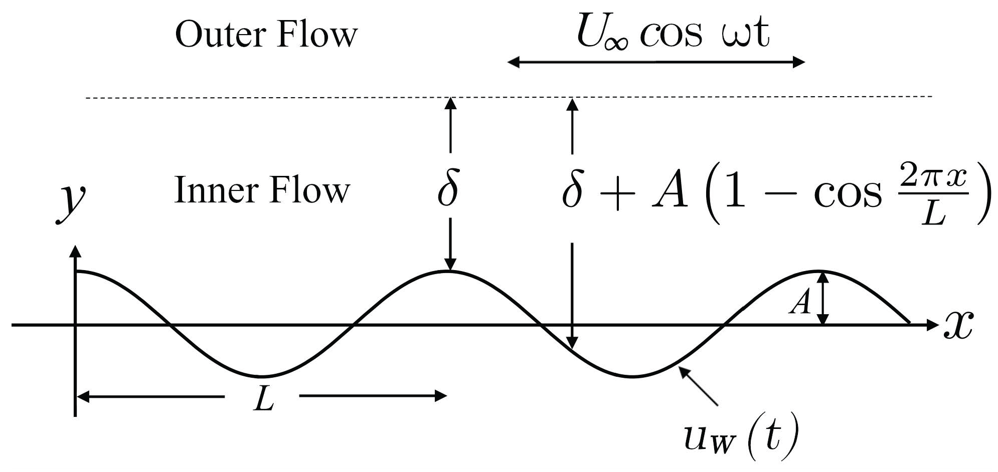
Figure 2.
First order axial velocity as a function of the transversal coordinate for different values. and .
Figure 2.
First order axial velocity as a function of the transversal coordinate for different values. and .
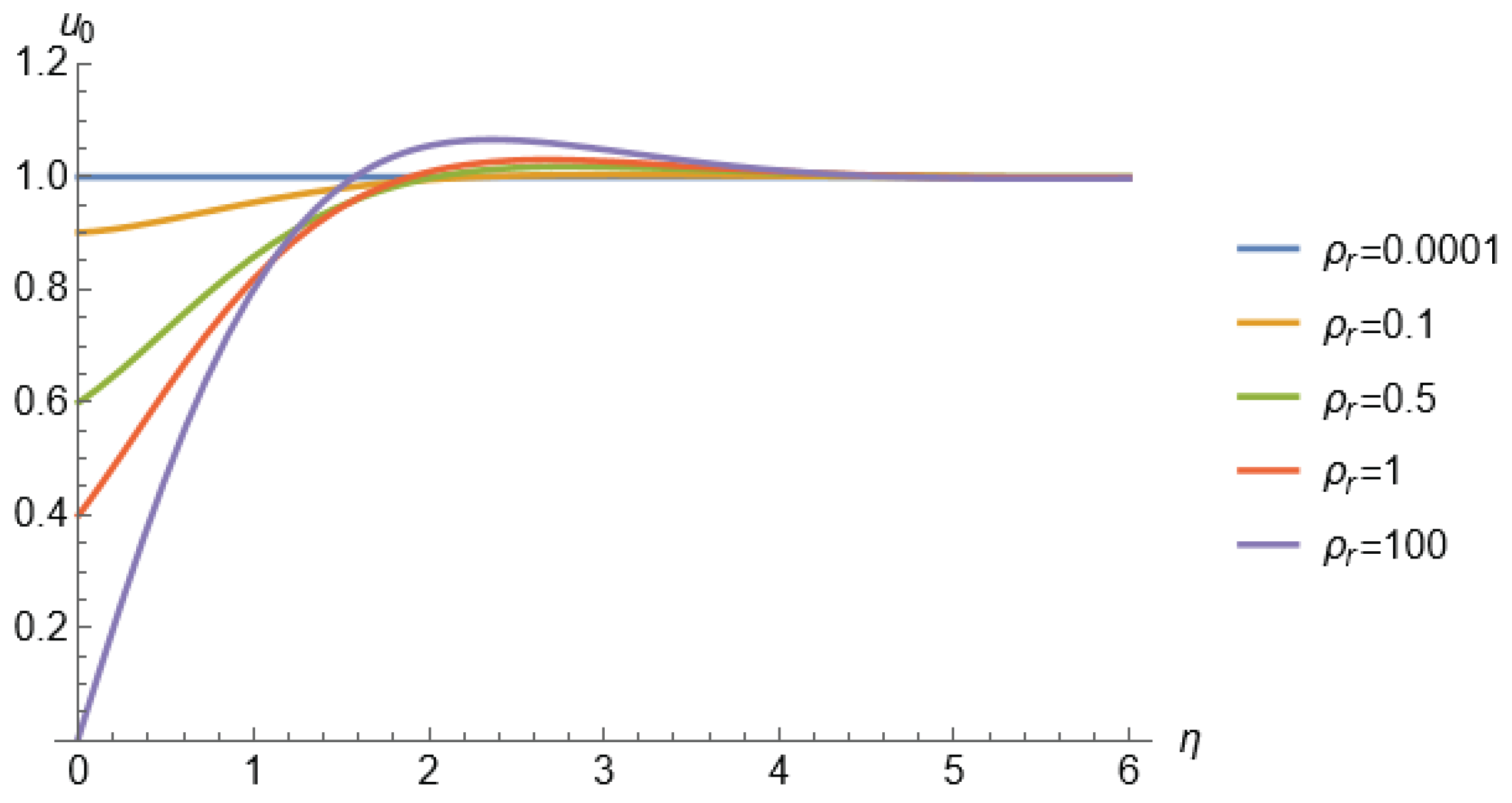
Figure 3.
First order axial velocity as a function of the transversal coordinate at different times with . a) Fixed-wall case, . b) Freely moving wall case, .
Figure 3.
First order axial velocity as a function of the transversal coordinate at different times with . a) Fixed-wall case, . b) Freely moving wall case, .
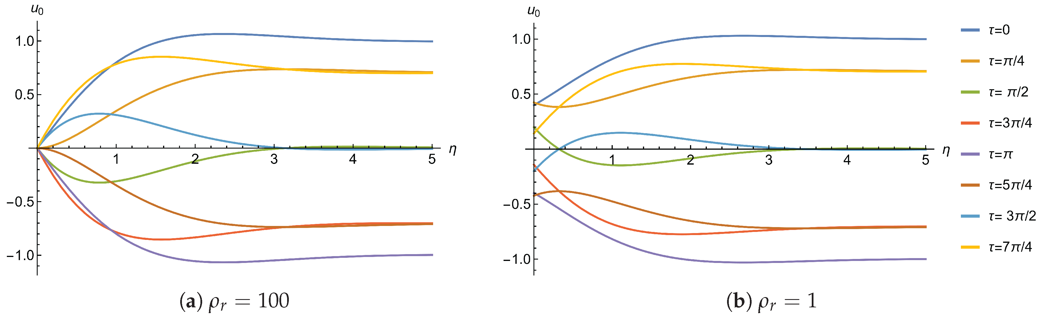
Figure 4.
Normalized as a function of for different values of . and .
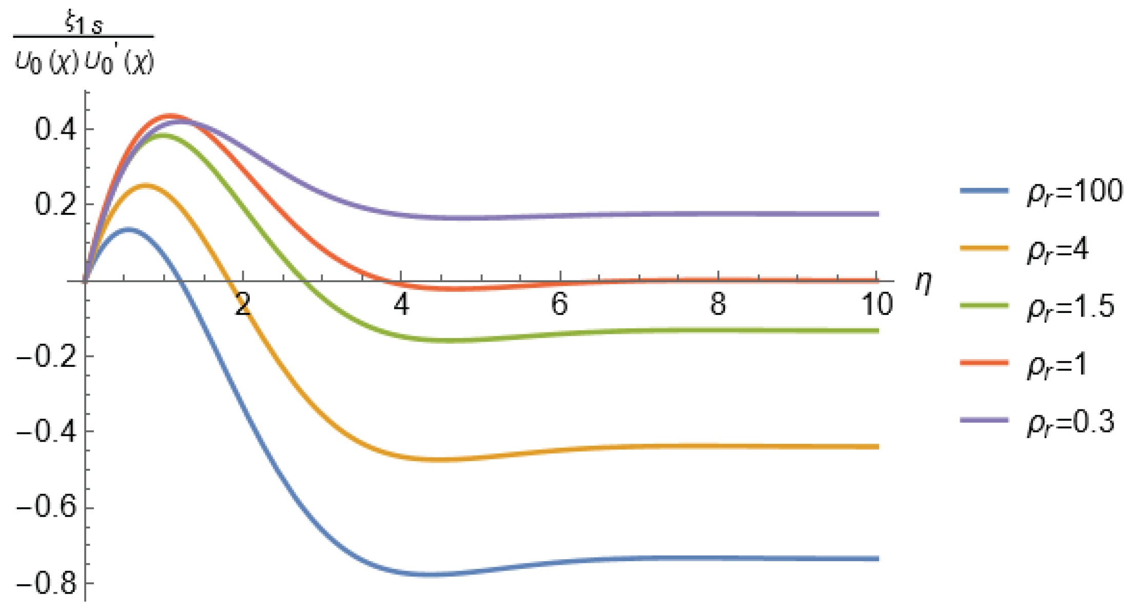
Figure 5.
Steady streaming velocity field superimposed on a background color vorticity map () over one wall wavelength, for different values and with .
Figure 5.
Steady streaming velocity field superimposed on a background color vorticity map () over one wall wavelength, for different values and with .
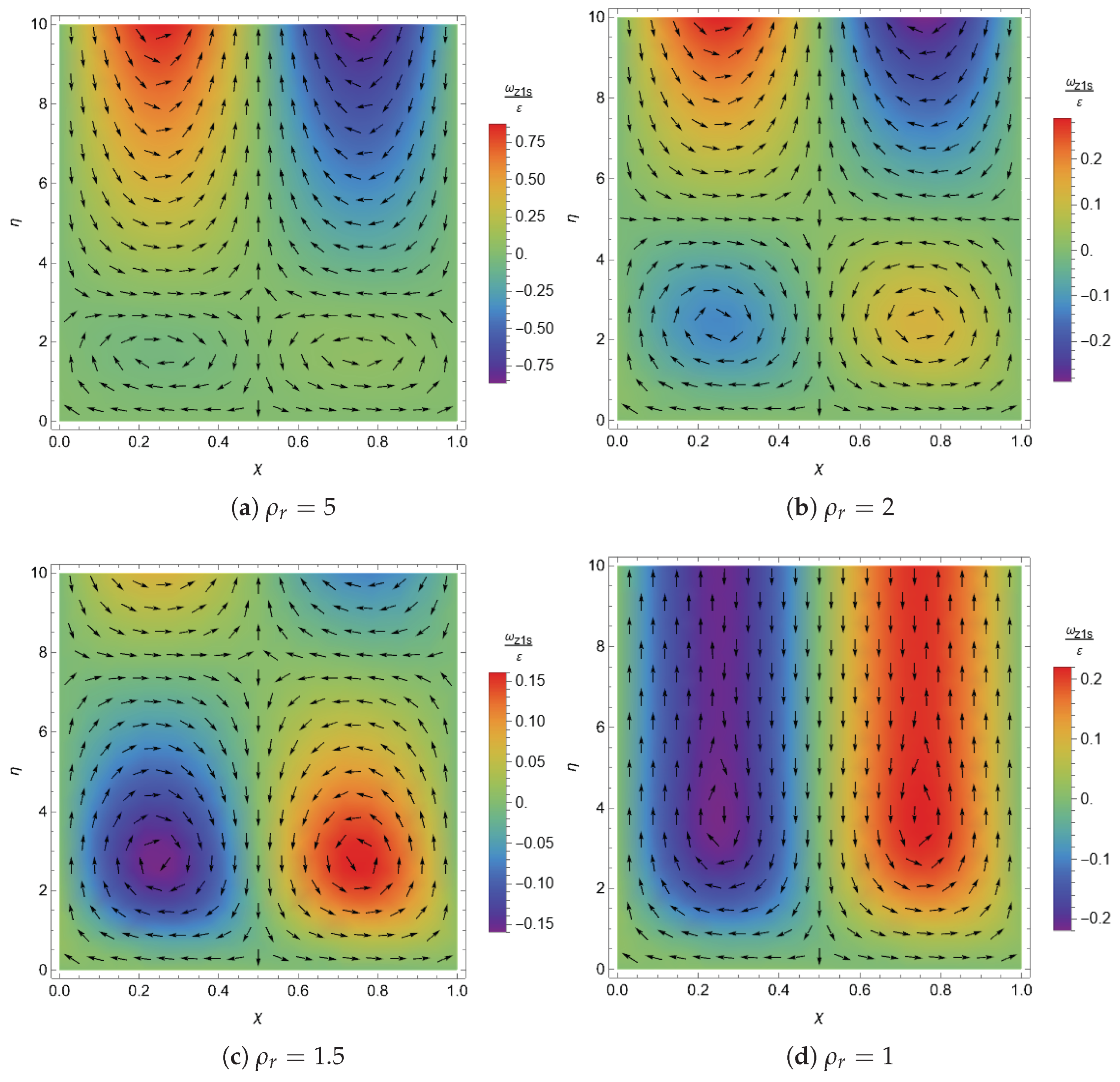
Figure 6.
Isometric view of the experimental device (not to scale). The upper-right panel: view of the plane from the PIV analysis. a) Function generator. b) Oscillatory electrical current. c) Floating plate. d) Laser source. e) Graphite electrodes. f) Camera. g) Permanent magnet. h) Oscillatory flow generated by the Lorentz force. i) Oscillatory motion of the floating plate. j) Magnetic field lines.
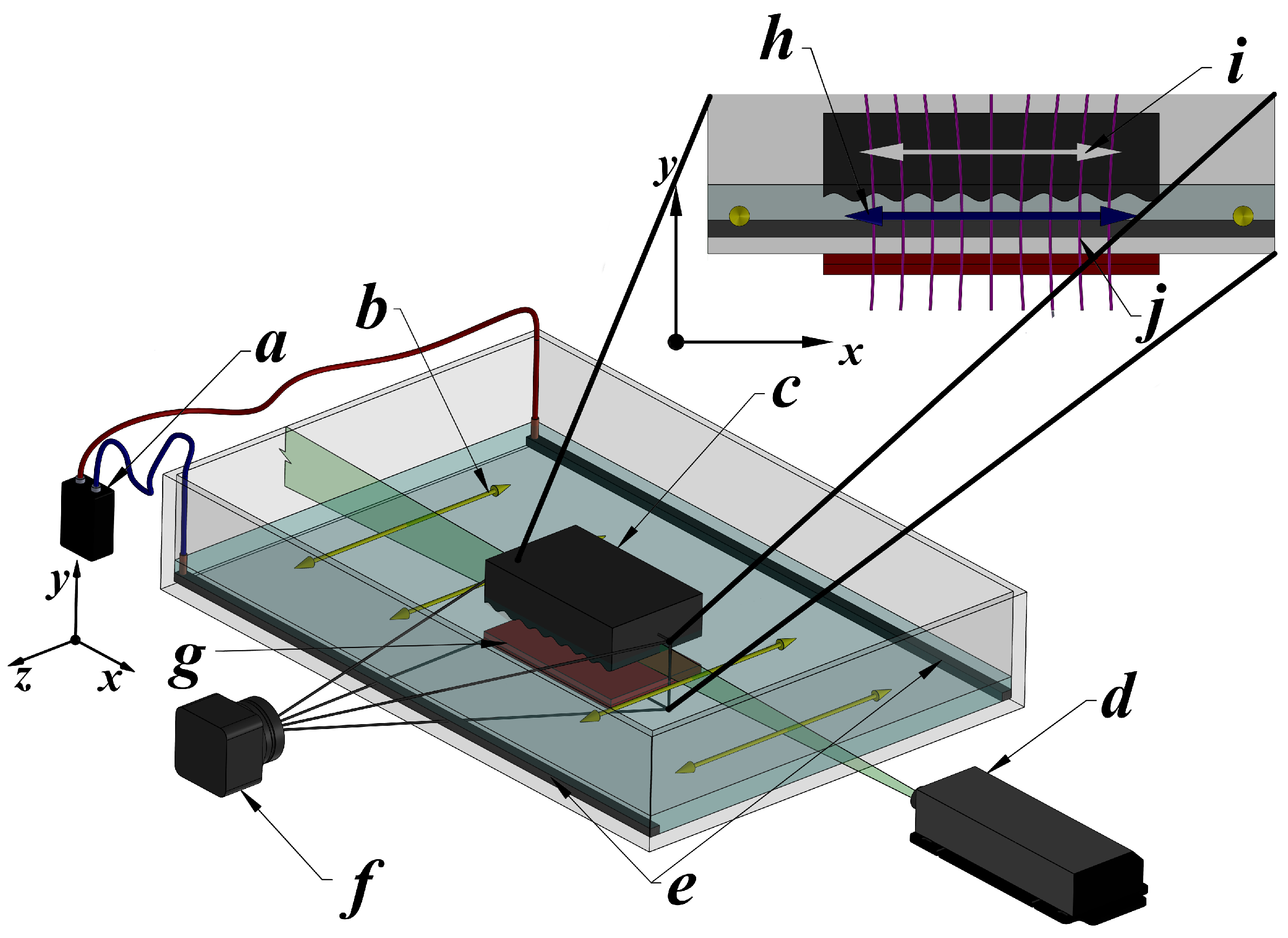
Figure 7.
One cycle time-averaged velocity field from PIV. a) Steady streaming, . b) Reverse steady streaming, .
Figure 7.
One cycle time-averaged velocity field from PIV. a) Steady streaming, . b) Reverse steady streaming, .
Disclaimer/Publisher’s Note: The statements, opinions and data contained in all publications are solely those of the individual author(s) and contributor(s) and not of MDPI and/or the editor(s). MDPI and/or the editor(s) disclaim responsibility for any injury to people or property resulting from any ideas, methods, instructions or products referred to in the content. |
© 2025 by the authors. Licensee MDPI, Basel, Switzerland. This article is an open access article distributed under the terms and conditions of the Creative Commons Attribution (CC BY) license (http://creativecommons.org/licenses/by/4.0/).
Copyright: This open access article is published under a Creative Commons CC BY 4.0 license, which permit the free download, distribution, and reuse, provided that the author and preprint are cited in any reuse.


