Submitted:
09 December 2025
Posted:
11 December 2025
Read the latest preprint version here
Abstract
The primary objective of the paper is to make a case that the evaluation of the expected returns in the Two-Envelope Paradox (TEP) is problematic due to the ill-defined framing of X and Y as random variables representing two identical envelopes, where one contains twice as much money as the other. In the traditional literature, when X is selected, Y is defined in terms of the amount of money x in X using the values y= x and y=2x with equal probability .5, and vice versa when Y is selected. The problem is that the event X=x stands for two distinct but unknown values representing the money in the two envelopes, say $θ and $2θ. This renders X and Y ill-defined random variables whose spurious probabilities are used to evaluate the traditional expected returns. The TEP is resolved by applying formal probability-theoretic reasoning to frame the two random variables in terms of the two unknown values {θ, 2θ}, giving rise to sound probability distributions, whose expected returns leave a player indifferent between keeping and switching the chosen envelope.
Keywords:
two-envelope paradox
; exchange paradox
; probability-theoretic reasoning
; random variables
; joint and marginal distributions
; expected returns
; axiomatic probability theory
1. Introduction
In a book entitled "The Waltz of Reason: the Entanglement of Mathematics and Philosophy" Sigmund (2023), pp. 185-187, brings out the ‘weird streak of probability’ by discussing two famous puzzles, the Monty Hall (or three doors) and the Two-Envelope (or exchange) paradoxes. A simple Google Scholar search reveals more than 34,000 citations for the former and more than 176,000 citations for the latter. Both problems are very beguiling because they are easy to understand with minimal mathematical knowledge and appear to raise issues that cut across different disciplines, including probability theory, statistics, logic, philosophy of science, economics, psychology, decision theory, and game theory. Despite their apparent simplicity, both problems involve formal probabilistic reasoning whose complexity is often underestimated; see Spanos (2019) on the complexity relating to the Monty Hall puzzle.
The discussion next focuses on the Two-Envelope Paradox (TEP), described by Sig-mund (2023), p. 186, as follows: “The quizmaster tells us that one of the envelopes contains a certain sum of money, and the other one twice that much. We pick an envelope, are allowed to open it, and see that it contains $40. Now the quizmaster offers us to exchange the chosen envelope with the other one, which has not been opened. Should we agree with the exchange?”
It should be noted that in certain variants of the problem, the player does not see the contents of the selected envelope, but that makes no difference to the main argument in this paper. Also, the discussion focuses on viewing this conundrum from the perspective of frequentist probability theory, but the results are also relevant when the TEP is viewed from a Bayesian perspective; see Christensen and Utts (1992), Lindley (2006).
2. The Traditional Expected Returns Evaluation of the TEP
The traditional account of the TEP views the two identical envelopes as random variables X and Y where the player selects one envelope and observes the value of X=x or Y=y, and derives the probability distribution of Y or X as a function of x or y, respectively, using the fact that one envelope contains twice as much money as the other envelope. That is, when envelope X contains $θ>0, envelope Y contains $2θ, and vice versa; .
Assuming that envelope X containing money x is selected, the traditional literature derives the probability distribution of Y in Table 1A by assigning the values y= and y=2x with equal probability .5 since the two envelopes are identical. When envelope Y is selected, the same thought process leads to the distribution in 1B.
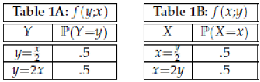
Evaluating the expected returns for each envelope, based on Tables 1A and 1B, yields:
These results imply that it would be rational for the player to always exchange the original envelope, irrespective of the values x and y. This is clearly fallacious, but the difficulty is pinpointing the flaw in the reasoning invoked that yields the result in (1).
The plethora of published papers proposing resolutions to this conundrum is a tes-tament to its puzzling complexity; see Nalebuff (1989), Linzer E. (1994), Rawling (1994), Broome (1995), Wagner (1999), Clark and Shackel (2000), Chalmers (2002), Dietrich and List (2004), Albers et al. (2005), Falk (2008), Falk and Nickerson (2009), Yi (2013), Vasudevan (2019), Portnoy (2020), Brock and Glasgow (2022), Hoffmann (2023) inter alia.
What all these papers have in common is that they take the probabilities in Tables 1A and 1B at face value and proceed to propose reasoned modifications of these probabilities that would change the expected returns evaluation to render the two envelopes equivalent. However, as argued next, the actual culprit behind the TEP is the framing of Y and X in terms of the values x and y. An exception is Gill (2021), who calls into question the numerous proposed resolutions of the TEP by arguing that: “There is no single resolution to the paradox of the type “so-and-so fails,” nor is there a unique explanation of what went wrong. Looking for one is illusory. Unless we take a broader perspective and say that the writer was attempting to do probability theory without understanding its concepts—let alone its rules—and therefore made serious errors by failing to draw distinctions that are essential in probability theory. TEP exemplifies the very reasons formal probability theory was developed. Philosophers who work on TEP without knowledge of modern (even elementary) probability theory are largely wasting their time; at best, they will reinvent the wheel.” (pp. 212-213)
The following discussion unfolds Gill’s insight by adhering to the rules and distinc-tions of formal probability theory to resolve the TEP.
3. Revisiting the Probabilistic Framing of the TEP
3.1. Questionable Features of the Traditional Framing
The key culprit behind the TEP is the framing of the envelopes X and Y as random variables using the events Y=y and X=x, denoting the money in these envelopes, to derive their probability distributions. This gives the misleading impression that the problem is straightforward by masking the fact that these random variables are ill-defined on probability theory grounds. Indeed, this framing raises two issues.
- (a)
- The first issue relates to the ambiguity of X=x and Y=y since x and y stand for two distinct but unknown values θ and 2θ. This renders Y and X ill-defined random variables whose distributions f (y; x) and f (x; y) in Tables 1A and 1B are spurious, being neither sound marginal nor conditional distributions.
- (b)
- The second issue is that the random variables X and Y are Identically Distributed (ID) but non-Independent since their respective values define two mutually exclusive events, calling into question the validity of Tables 1A and 1B.
As argued next, (a)-(b) can be addressed by reframing the random variables X and Y in terms of the unknown values {θ, 2θ}, which secure well-defined joint and marginal distributions that resolve the TEP. Any superficial similitude between the two framings, in terms of {x, y} vs. {θ, 2θ}, is more apparent than real!
3.2. Formal Probabilistic Framing of the Random Variables in the TEP
Probability theory became part of mathematics when Kolmogorov (1933), p. 1, pro-posed an axiomatic approach:
“The theory of probability, as a mathematical discipline, can and should be developed from axioms in exactly the same way as Geometry and Algebra. This means that after we have defined the elements to be studied and their basic relations, and have stated the axioms by which these relations are to be governed, all further exposition must be based exclusively on these axioms, independent of the usual concrete meaning of these elements and their relations.”
The first principle of probability theory is to ensure that the random variables, X and Y are well-defined on the same probability space (S, F, P(.)) where (Williams, 2001):
- [i] S denotes the set of all possible distinct outcomes.
- [ii] F comprises the events of interest as subsets of S in the form of a sigma-field, i.e. F should be closed under countable unions, intersections, and complementations.
- [iii] P(.)→[0, 1] is a set function assigning probabilities to all elements in F, defined by the three Kolmogorov axioms.
- [iv] In the context of (S, F, P(.)), a discrete random variable Z(.) is a function from S to R, such that, all events of the form A(s):={s: Z(s)=z}∈F, ∀z∈RZ, where R denotes the real line and RZthe range of values of Z(.).
In the case of the TEP, there are two distinct possible outcomes, say S={s1, s2}, entail-ing that the relevant field (finite sigma-field) is F={S, ∅, s1, s2}, where s1 ∪ s2=S and s1 ∩ s2=∅-the empty set. The two relevant random variables are defined as follows:
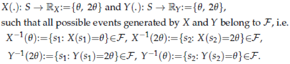
The second principle of probability theory is to distinguish clearly between the random variables X and Y and their values x and y since non-degenerate random variables take more than one value, and there is nothing random about these values.
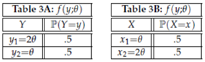
The next important issue is to ascertain, before any probabilities are assigned, is whether the two random variables X and Y are Independent. In light of the fact that when X contains $θ, Y must contain $2θ, and vice versa, X and Y are dependent. This suggests that to account for their dependence, one needs to derive their joint distribution f (x, y; θ) shown in Table 2. The two marginal distributions, f (x; θ) and f (y; θ), shown on the side and bottom of the table, are derived by summing over rows and columns, respectively.
The dependence between X and Y can be affirmed by showing that:

The two marginal distributions in Tables 3A and 3B affirm that X and Y are ID.
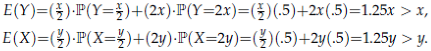
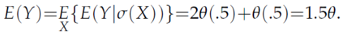
Using (3) one can evaluate the expected returns from envelopes Y and X to be:
rendering them identical in terms of θ. This suggests that a player would be indifferent between keeping and exchanging the original envelopes, unriddling the TEP. It also makes intuitive sense in terms of the expected returns evaluation based on the sum of $3θ. The result in (4) belies the traditional result in (1), questioning the spurious probabilities in Table 1A, stemming from the improper framing of the random variables X and Y.
E(Y)=.5(2θ)+.5θ=(1.5)θ, E(X)=.5θ+.5(2θ)=(1.5)θ,
Potential objection. One could question the above derivations in Table 2 and Table 3A and 3B on formal probability-theoretic grounds, given that θ is unknown, rendering the random variables X and Y latent. As shown in Appendix A, the above results are affirmed by conditioning on the field generated by X and Y to account for {θ, 2θ} being latent.
4. Conclusions
A case has been made above that the TEP is not a paradox but a misapplication of formal probability theory. The misapplication arises from using the event X=x to define Y as a function of x and vice versa. This renders the two random variables ill-defined since x and y stand for two distinct outcomes θ and 2θ. That is, using the values y= and y=2x, together with x= and x=2y instead, gives rise to the two spurious distributions in Tables 1A-1B engendering the TEP.
The TEP is resolved on formal probability-theoretic grounds when both random variables X and Y are defined on the same probability space (S, F, P(.)), where S={s1, s2}, and F={S, ∅, s1, s2}. Defining the random variables X and Y on in terms of the latent {θ, 2θ}, relating to {s1, s2}, gives rise to a well-defined joint distribution f (x, y; θ) and the ensuing marginal distributions, f (x; θ) and f (y; θ) in (3). Using these marginal distributions to evaluate the expected returns in (4) leaves the player indifferent between switching and retaining the original envelope, puzzling out the TEP. This result is also affirmed by accounting for the fact that the two random variables X and Y are, in essence, latent.
Funding
This research received no external funding.
Institutional Review Board Statement
Non-applicable.
Informed Consent Statement
Non-applicable.
Data Availability Statement
No data are used
Conflicts of Interest
The author declares no conflict of interest.
Abbreviations
The following abbreviations are used in this manuscript:
| TEP | Two-Envelope Paradox |
Appendix A. Conditioning on Latent Random Variables
A more circuitous but probabilistically elucidating way to reach the result in (4) is to treat both random variables as latent since their values in Table 2 are unobservable, and deal with the ambiguity of the event X=x using the conditional expectation E(Y|σ(X)), where σ(X)={S, ∅, X=θ, X=2θ}, denotes the field generated by X, and analogously for E(X|σ(Y)). The defining relation for E(Y|σ(X)) takes the generic form (Billingsley, 1995, p. 445):

To evaluate E(Y|σ(X)) one needs both conditional distributions relating to outcomes x=θ and x=2θ, whose singularity stems from their mutual exclusiveness:
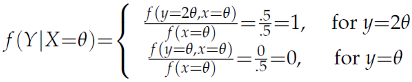
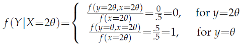
Hence, E(Y|σ(X)) defines a random variable of the form:

where 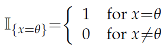 is the indicator function.
is the indicator function.To derive the expected winnings of exchanging envelopes one needs E(Y) which can be derived from (8) using the law iterated expectations (Williams, 1991):
Reversing the roles of X and Y we can define E(X|σ(Y)) and derive the analogous result:

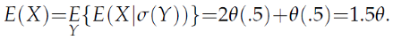
The results in (9) and (11) affirm those in (4).
References
- Albers, C.J, B.P. Kooi and W. Schaafsma (2005) “Trying to resolve the two-envelope problem”, Synthese, 145(1): 89-109.
- Billingsley, P. (1995) Probability and Measure, 3rd edition, Wiley, NY.
- Brock, S. and J. Glasgow (2022) “The paradox paradox”, Synthese, 200(2): 83.
- Broome, J. (1995), “The two envelope paradox,” Analysis, 55: 6-11.
- Chalmers, D.J. (2002), “The St. Petersburg two-envelope paradox,” Analysis, 62: 155-157.
- Clark, M., and N Shackel (2000) “The two envelope paradox”, Mind, 109: 415-442.
- Christensen, R. and J. Utts (1992) “Bayesian resolution of the “exchange paradox”, The American Statistician, 46(4), 274-276.
- Dietrich, F., and C. List (2004) “The two-envelope paradox: An axiomatic approach,” Mind, 114: 239-248.
- Falk, R. (2008) “The unrelenting exchange paradox”, Teaching Statistics, 30(3), 86-88.
- Falk, R. and R. Nickerson. (2009), “An inside look at the two envelopes paradox,” Teaching Statistics, 31: 39-41.
- Gill, R.D. (2021) “Anna Karenina and The Two Envelopes Problem”, Australian & New Zealand Journal of Statistics 63(1): 201–218.
- Hoffmann, C.H. (2023) “Rationality applied: resolving the two envelopes problem”, Theory and Decision, 94(4): 555-573.
- Kolmogorov, A.N. (1933) Foundations of the theory of Probability, 2nd English edition, Chelsea Publishing Co. NY.
- Lindley, D.V. (2006) Understanding Uncertainty, Wiley, NY.
- Linzer E. (1994) “The Two Envelope Paradox”, The American Mathematical Monthly 101(5): 417-419.
- Nalebuff, B. (1989) “Puzzles: the other person’s envelope is always greener,” Journal of Economic Perspectives, 3: 171-181.
- Portnoy, S. (2020) “The Two-Envelope Problem for General Distributions”, Journal of Statistical Theory and Practice, 14: 1-15.
- Prasanta S.B., D. Nelson, M. Greenwood, G. Brittan and J. Berwal (2011), “The logic of Simpson’s paradox”, Synthese 181:185–208, DOI 10.1007/s11229-010-9797-0.
- Rawling, P. (1994). “A Note on the Two Envelopes Problem”, Theory and Decision, 36: 97–102.
- Sigmund, K. (2023) The Waltz of Reason: the Entangelment of Mathematics and Philosophy, Basic Books, NY. 85.
- Spanos, A. (2019), Probability Theory and Statistical Inference: empirical modeling with observational data, Cambridge University Press, Cambridge.
- Vasudevan, A. (2019) “Biased information and the exchange paradox”, Synthese, 196(6): 2455-2485.
- Wagner, C.G. (1999) “Misadventures in conditional expectation: The two-envelope problem”, Erkenntnis, 233-241. [CrossRef]
- Williams, D. (2001) Weighing the odds: A course in probability and statistics, Cambridge: Cambridge University Press.
- Yi, B.U. (2013) “Conditionals and a Two-envelope Paradox”, The Journal of Philosophy, 110(5): 233-257.

Table 2.
f (x, y; θ).
| X \ Y | θ | 2θ | f (x; θ) |
| θ | 0 | .5 | .5 |
| 2θ | .5 | 0 | .5 |
| f (y; θ) | .5 | .5 | 1 |
Disclaimer/Publisher’s Note: The statements, opinions and data contained in all publications are solely those of the individual author(s) and contributor(s) and not of MDPI and/or the editor(s). MDPI and/or the editor(s) disclaim responsibility for any injury to people or property resulting from any ideas, methods, instructions or products referred to in the content. |
© 2025 by the authors. Licensee MDPI, Basel, Switzerland. This article is an open access article distributed under the terms and conditions of the Creative Commons Attribution (CC BY) license (http://creativecommons.org/licenses/by/4.0/).
Copyright: This open access article is published under a Creative Commons CC BY 4.0 license, which permit the free download, distribution, and reuse, provided that the author and preprint are cited in any reuse.


