
Submitted:
07 December 2025
Posted:
10 December 2025
You are already at the latest version
Abstract
The distribution of prime numbers has long been a central topic in analytic number theory. The Prime Number Theorem (PNT), which states that a number of primes less than x is \( x/log(x) \), provides a foundational understanding of this phenomenon. The further study of deep insights has led to the Riemann Hypothesis (RH), which implies explicit bounds on the error term in the PNT, thus enhancing the precision of the results derived from it. In this work, an algorithm is proposed for the estimation of the prime-counting function by counting the number of composite numbers eliminated during the sieving of the odd-number sequence. By applying this approach, it was found that variations in the length of the odd-number sequence during removal of composite numbers follow an oscillation pattern governed by the sinc function. Further analysis of such oscillations suggests that the function \( π(x) \) is composed of two terms: the main term, which makes the largest contribution to the distribution of the primes, and the error term, which is responsible for the accumulation of errors during the calculation of the \( \text{sinc} \) function values up to the limit \( m \), defined as \( √x /2 \). This leads to the proposal that the bound coefficient of the error term should be equal to \( √x/log x \), which is correlated with an estimate of this coefficient derived under the assumption of the truth of the RH. We hope that this perspective stimulates future work toward formalizing this approach to uncover deeper connections to the zeta function and prime number theory at large scale.
Keywords:
Prime Number Theory (PNT)
; bound error term
; Riemann Hypothesis (RH)
; sieving algorithm
1. Introduction
A prime number (or just prime) is a natural number greater than 1 that is not a product of two smaller natural numbers. Primes are central in number theory because of the fundamental theorem of arithmetic: every natural number greater than 1 is either a prime itself or can be factorized as a product of primes that is unique up to their order. There are infinitely many primes, as demonstrated by Euclid around 300 BC using a very elegant and simple proof.
But how many prime numbers are there up to a given number? Consider the prime-counting function denoted by , which is defined as the number of prime numbers less than or equal to x for any real number x. In 1849, in a letter to the German astronomer Johann Franz Encke [1], Carl Friedrich Gauss made a note suggesting that the number of prime numbers less than or equal to x is:
The Formula (1) later became known as the Prime Number Theorem (PNT). Legendre conjectured in 1796 that there exists a constant B such that satisfies:
B is known as Legendre’s constant. Regardless of its exact value, the existence of this constant implies the Prime Number Theorem. In 1849 Pafnuty Chebyshev proved that if the limit B exists, it must be equal to 1.
The PNT then states that is a good approximation for (where log here means the natural logarithm), in the sense that the limit of the quotient of the two functions and , as x increases, is 1:
In a handwritten note on a reprint of his 1838 paper “Sur l’usage des séries infinies dans la théorie des nombres” [2], which he mailed to Gauss, Gustav Lejeune Dirichlet conjectured (under a slightly different form appealing to a series rather than an integral) that an even better approximation to is given by the offset logarithmic integral function , or the Eulerian logarithmic integral, defined as:
where is defined as:
Based on this, the PNT can also be written as:
In 1859, Bernhard Riemann in a short but monumental paper titled “Über die Anzahl der Primzahlen unter einer gegebenen Größe” (“On the Number of Primes Less Than A Given Magnitude”) introduced the Riemann zeta function, defined for complex numbers at as (7):
This function had already been studied by Euler, but for real values of s, and Riemann extended its domain to complex numbers and explored its analytic properties. Crucially, he showed that the distribution of prime numbers is intimately connected to the behavior of the zeros of the zeta function (the values of s for which ). In particular, Euler discovered in 1737 the connection between the zeta function and prime numbers by proving that:
In 1896, Jacques Hadamard and Charles Jean de la Vallée-Poussin independently proved the PNT using complex analysis and properties of the zeta function, specifically, by showing that all non-trivial zeros of the zeta function lie within the critical strip . Riemann himself proposed that all non-trivial zeros of the zeta function lie on the critical line . This bold conjecture, now known as the Riemann Hypothesis (RH), remains one of the most important unsolved problems in mathematics. In 1914, Godfrey Harold proved that has infinitely many real zeros. More than 10 trillion (i.e. ) non-trivial zeros of the Riemann zeta function have been verified, and all of them lie on the critical line [3].
The connection between the Riemann zeta function and the prime-counting function is one reason the Riemann hypothesis has considerable importance in number theory: if established, it would yield a far better estimate of the error involved in the prime number theorem. More specifically, Helge von Koch showed in 1901 that if the RH is true, the error term in the PNT can be expressed as:
where O is a big O notation. This is in fact equivalent to the RH.
The constant involved in the big O notation was estimated in 1976 by Lowell Schoenfeld [4], assuming the RH is true:
for all . For the Chebyshev prime-counting function , which is determined as:
a similar bound to (10) can also be derived:
From the formulas above, it can be seen how strongly the assumption of the truth of the Riemann Hypothesis influences the Prime Number Theorem, particularly in estimating the error term in the distribution. If RH is true, then the error term in the PNT is bounded by the factor .
In this article, an approach to decomposition of into a dominant term and an error term based on sequential elimination of the composite numbers up to number N is described. This formulation offers a new lens for interpreting the prime distribution and invites further exploration into the analytic and statistical nature of these components. Connections to classical approximations, such as Li(x) and the corresponding error term, and potential links to the zeros of the Riemann zeta function, are also briefly discussed.
2. Estimation of the Prime-Counting Function by Applying of Composite Numbers Elimination
Start by considering the Sieve of Eratosthenes algorithm. It is a simple algorithm to find all prime numbers up to a given number N. The main idea of this algorithm is to sequentially remove all composite numbers that are divisible by 3, 5, 7, and so on. The numbers that remain unmarked are primes. But the Sieve of Eratosthenes is an algorithm, not an analytical formula. Although it is effective in practice for finding all prime numbers up to a given number N, it does not produce an exact analytical expression for the prime-counting function . The difficulty in obtaining an analytical formula is closely related to the complexity of implementing the sieving of numbers. Consequently, it becomes necessary to explore alternative computational or theoretical approaches in an effort to derive such a formula. In the following, the approach to approximate the calculation of using analytic functions is presented.
Returning to the discussion of the Sieve of Eratosthenes algorithm, our objective is to quantify the number of composite numbers eliminated during the sieving process. To achieve this, we formulate an algorithm that computes the number of elements removed at each iteration, and after that we analyze the resulting pattern. Specifically, we examine how the number of remaining odds evolves throughout the procedure. Beyond a certain threshold, this amount stabilizes, indicating that only prime numbers remain. The number of these residual primes corresponds to the prime-counting function, denoted by the function.
The pseudocode for this algorithm can be expressed as follows:
- 1) N = 5000
- 2) odds = list(3, N, step 2)
- 3) length_changes = [empty list]
- 4) i = 1
- 5) while (i < (some condition)):
- (6) L = list(3∗(2∗i + 1), N, 2∗(2∗i) + 1)
- (7) odds = difference(odds, L)
- (8) length_changes.append(len(odds)(before)
- - len(odds)(after))
- (9) i = i + 1
This is how the program can be constructed in a programming language.
- In line (1), a number is set — for example, N = 5000.
- In line (2), a list is created that contains all odd numbers from 3 to N.
- Then, on line (3), an empty list is initialized. This list will track how the length of the odd-number list changes as the composite numbers are removed.
- In block (5), a while loop runs at each step i (starting from 1), generating all the composite numbers divisible by from to N (line (6)), while a certain condition holds (the exact condition will be discussed in detail later).
-
Lines (7) and (8) are crucial:
- -
- Line (7) performs a set difference between the list of remaining odd numbers and the composite numbers generated at the current step i. This effectively removes from the list all composite numbers divisible by
- -
- Line (8) calculates how the length of the odd-numbers sequence changes, and this difference is stored in the list.
- Finally, line (9) proceeds to the next iteration i.
The array after running this pseudocode contains all primes up to N, and its length is the total number of primes less than or equal to N, which is denoted as .
However, it is not necessary to find all the composite numbers for every step i up to N, because after a certain point no new composite numbers are generated, and the length of the odd-numbers array stops changing. Let this threshold be denoted as m. Then the condition in the while loop can be rewritten as .
To determine m, we proceed with the following reasoning. The rows and columns in Figure 1 contain all numbers divisible by each odd number (each odd number can be generated with formula by letting i be equal to 1, 2, 3, etc.) within the range from 3 to N (we set in Figure 1 for simplicity).
- The first row contains all numbers divisible by 3, the second one by 5, etc.
- The table is symmetric with respect to the main diagonal, where the entries correspond to the squares of ().
- All composite numbers - whose total count is to be determined - are located in one half of the matrix, along with diagonal elements that represent perfect squares.
Based on Figure 1, the number of composite numbers can be determined by simple reasoning:
- The number of values divisible by 3 is approximately , considering only odd numbers.
- The count of values divisible by 5 is , since 15 has already been counted.
- The count of values divisible by 7 is , as 21 and 35 have already been included on the opposite side of the diagonal and should not be double-counted.
In general, for each successive odd number i, the number of previously counted values to subtract is . The calculation continues until the subtraction term is equal to the number , from which it is subtracted.
This simple reasoning can be expressed as follows:
Where corresponds to the threshold m.
And finally:
We define m approximately as . The value m serves as a threshold beyond which the removal of composite numbers no longer contributes to the enumeration of composite numbers.
The pseudocode can then be rewritten as:
- 1) N = 5000
- 2) odds = list(3, N, step 2)
- 3) length_changes = [empty list]
- 4) i = 1
- ∗) m = N/(2(2i+1))
- 5) while (i < m):
- (6) L = list(3∗(2∗i + 1), N, 2 ∗ (2∗i)+1)
- (7) odds = difference(odds, L)
- (8) length_changes.append(len(odds)(before)
- - len(odds)(after))
- (9) i = i + 1
- (∗∗) m = N/(2(2i+1))
Two additional lines of code are introduced. The added line initializes the parameter m, which is subsequently reassigned to a new value (in another added line ()). Upon execution of the modified code, a sieving procedure can be applied to the list of odd numbers, effectively isolating the prime elements for an arbitrary N.
Figure 2 exhibits a notable oscillatory pattern and illustrates how the length of the odd number sequence evolves as the composite numbers are progressively removed. This behavior closely mirrors the characteristic form of the sinc function, defined as
To explore an approximation of the prime-counting function using the sinc function, we begin by considering the following definition:
The function (20) exhibits oscillatory behavior and its frequency is governed by the parameter w. In the context of the sieving of composite numbers, specifically those divisible by 3 — we can naturally associate this frequency w with the reciprocal of the divisor, that is, . This natural choice reflects the periodicity of the removal of multiples of 3 in the sieve process. To appropriately scale the amplitude of the sinc function for our application, we introduce a normalization factor. Empirically, this factor can be determined approximately equal to (its determination is based on a direct comparison of variations of the length of the odds array depicted in a figure (2) with the behavior of the sinc function):
Since the sinc function inherently oscillates between positive and negative values, and the sieving process involves the removal (not addition) of elements, we apply a modulus operation to ensure the non-negativity of the number of items removed. This transformation ensures that the function contributes only to the exclusion of composite numbers. Combining these components, the function can be rewritten as:
The function (22) should start from . By definition, . However, in our case, represents the number of the composite numbers divisible by 3, and this value should be subtracted initially. Therefore, formally we can define .
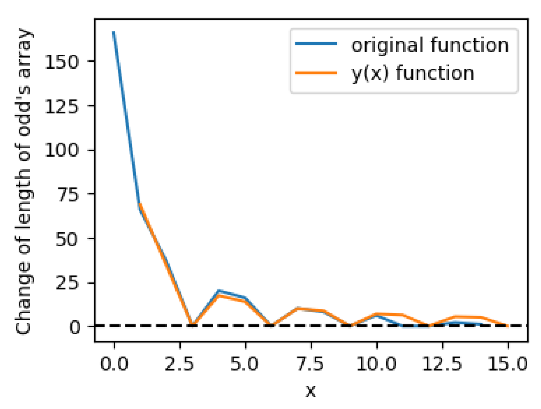
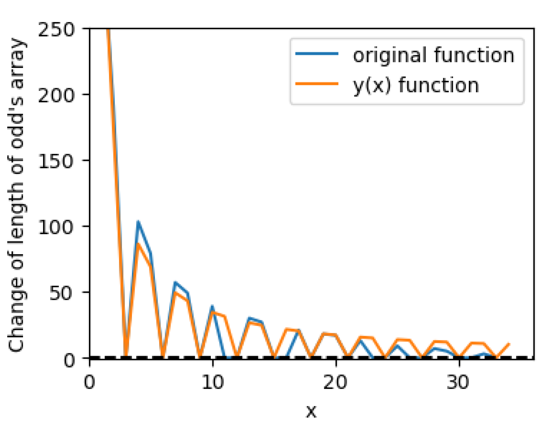
Plot a graph of the original function that calculates the variation in the length of an odd number sequence according to the pseudocode, along with the function (for N = 5000) (see Figure 3 and the magnified image (Figure 4). Now we can compare the behavior of the original function (as we saw previously in Figure 2) and the function (22). These two functions demonstrate very similar oscillation behavior; this leads one to believe that these functions are interconnected in some way. Note that upon magnifying the image, it becomes evident that the divergence between these functions grows with increasing i; however, we will defer a detailed study of this phenomenon to future work.
In case of , the function fairly accurately follows the original function. If we compare the actual variations of odd-array’s length while removing the composite numbers and variations which are calculated by :
1) Original variations: [66, 37, 0, 20, 16, 0, 10, 8, 0, 6, 0, 0, 2, 1]
2) Calculated variations: [68, 34, 0, 17, 13, 0, 9, 8, 0, 6, 6, 0, 5, 4, 0]
Figure 5.
The original function (blue line) of variations of odd numbers during of elimination of composite numbers (these variations are calculated according to the pseudocode and are hold in the list (lines 3 and 8 in the pseudocode)), and the function (orange line) defined as (22) for ).
Figure 5.
The original function (blue line) of variations of odd numbers during of elimination of composite numbers (these variations are calculated according to the pseudocode and are hold in the list (lines 3 and 8 in the pseudocode)), and the function (orange line) defined as (22) for ).
The variations in the actual length of the odd-numbers array for and the length calculated using the function are quite similar. If we calculate the number of primes up to 1000 by eliminating composite numbers according to the original algorithm (i.e., by applying the direct sieving algorithm), and then calculate the number of primes using the function for , we get the following results:
Calculation of primes by application of a direct sieving algorithm (as pseudocode describes):
Calculation of primes with function :
The actual number of primes is 167; the calculated number of primes with function is 169.
The variations of odds-array’s length calculated by direct calculation and with function are very similar. These findings imply that these two functions can exhibit correlated behavior or share underlying structural properties.
Now, rewrite the calculation the number of primes up to a given number N using function’s representation by a Formula (22)):
The subsequent analytical step involves considering that the original function, designed to evaluate changes in the length of the odd number array, yields zero at step i when is not a prime number. Consequently, the function should be redefined to include only those indices i for which , where p is a prime. The summation process must therefore be restricted to prime-valued terms. However, given that elements divisible by 3 have already been excluded in a prior step, the primality condition must be verified for the subsequent value , ensuring accurate filtration of non-prime contributions. This constraint must be incorporated into the formulation. Consequently, the revised expression should enforce the primality of () as a necessary condition for inclusion in the summation.
where , indicating that the summation is restricted to prime numbers only; the upper bound of the summation is defined by , which specifies the limiting value to which the summation is carried out.
The Formula (24) is an important one. First, we subtract all even numbers from N (their total value is ), then all numbers that are divisible by 3 (their total value is ∼), and finally we perform a sequential subtraction of all values , with the condition that the number should be prime.
However, the function (24) yields an approximate solution of rather than an exact value. To reflect this, in the Formula (24) can be reformulated as follows:
In Formula (25), can be interpreted as a simple but dominant function that is very close to the real value of . Based on this, we can decompose the function defined in (24) into two constituent components:
Let denote the dominant component that closely approximates the variations in the length of the array of odd numbers, and let represent an oscillatory error value corresponding to the variation at the step (). At this stage, we are not concerned with the explicit analytical forms of and ; rather, we assume the existence of such functions that capture the described behavior.
Decompose the function into two distinct components:
The term represents the dominant component which we denote as , and the term represents the error component responsible for capturing the error behavior, which we denote as :
Since summation in (29) is restricted to prime numbers, we utilize the Prime Number Theorem (PNT) to estimate a number of terms in the sequence in . Specifically, the number of primes up to m can be approximated by . This approximation allows us to estimate the number of terms involved in the summation over primes up to the limit m:
And now rewrite as:
where is a function of N that accounts for a mean error across all and is an estimation of a total number of terms in .
Finally, rewrite as

Formula (32) implies that the prime-counting function can be expressed in two terms: a function , which closely approximates - and an average error component , representing the cumulative deviation from the expected distribution. Furthermore, the error term is expected to exhibit an oscillatory behavior, analogous to that of the sinc function, reflecting the inherent fluctuations in the distribution of prime numbers. For the purposes of this analysis, we shall abstract away the intrinsic nature of the function . It is essential that represents the dominant contribution to and represents the error term.
Formula (32) is the most significant implication derived from the preceding analysis. In fact, it allows us to conclude that the error term in the prime-counting function should have a behavior similar to regardless of the function, where the function represents an oscillatory error term with bound coefficient .
Return to the Chebyshev prime-counting function , which was described in the introduction (11). 35 years after Riemann published his paper, the German mathematician Hans von Mangoldt studied and found a relatively simple explicit formula for it [5]:
This formula consists of four terms: the first one is simply x, the second one is a constant, the third one , which involves the sum of trivial zeros of the zeta function and becomes negligible for large value of x, and the fourth and the important one is the sum of over all the non-trivial zeros of the zeta function.
Divide equation (12) by :
From (33) after exclusion of and an expression for can be rewritten as a relatively simple explicit formula:
The expression (40) shows that is estimated as minus the sum of all non-trivial zeros of the zeta function divided by . If RH is true, all non-trivial zeros have a real part that is , and thus each non-trivial zero can be written as .
Using this, rewrite the sum :
The function in (41) is a sum of imaginary parts of the non-trivial zeros of the zeta function.
Based on (41), the expression for the sum can be written in the simplified version:
And finally, Formula (40) can be written as:
where is equal to the sum of imaginary parts of non-trivial zeros of the zeta function .
Now we have two formulas for :
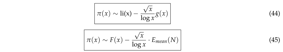
The formula (45) is derived from the analysis of oscillations of the length of odd-numbers array, where is an oscillation function and is a function that is close to the true value of and can be considered as an analog for li(x) (because function li(x) is the closest known approximation of the prime-counting function). More interesting is a term which aggregates a sum of imaginary parts of non-trivial zeros.
If we rewrite as:
and then the sum of non-trivial zeros can be rewritten as next:
The function also has an oscillating behavior, because it can be represented by Euler’s formula:
Riemann’s hypothesis expresses the error in the prime number theorem as the sum of waves with wavelength determined by the locations of the zeros of . In [7] the following approximate expression is given to demonstrate this:
The zeros of the Riemann zeta function are placed so precisely that they anticipate the locations of the primes. Moreover, they do it through the Fourier series type term in (50) in which the values of the zeros determine both the amplitude and the wavelength - analog of the sine-log waves. If the Riemann hypothesis is false, the Formula (50) would be marred with more complicated coefficients for the sines that are functions of x, which are different from .
Regrouping the terms, we can rewrite our formula (45), which was previously derived from the analysis of variations of the odd number quantity during the removal of composite numbers, in the following form of (50):
The function is the mean of errors up to the limit m (see Formula (31)) and also has sinusoidal oscillation behavior in the form of functions sinc, as we saw previously (26). Based on the similarity of (50) and (51), we can propose that this function describes a sum of imaginary parts of non-trivial zeros of the zeta function. The more interesting for us is that this formulation concludes that the coefficient in our Formula (51) has a value of , which we have derived from an estimation of the limit to count the composite numbers, as we established earlier. But, in formulas (47) and (50), this coefficient is derived from the proposal that all non-trivial zeros have a real part equal to , as proposed by the Riemann Hypothesis. Moreover, the similarity of formulas (51), (50) and (44) may also provide supporting evidence for the validity of the RH.
3. Conclusions
In this work, an algorithm for calculating the prime counting function is proposed by determining the number of odd numbers remaining after removing the composite ones. This method generalizes the classical Sieve of Eratosthenes algorithm by not only identifying and excluding composite numbers but also quantifying the number of such eliminations during the sieving process. By applying this approach, it was found that these variations follow an oscillation pattern governed by the sinc function. The further analysis of such oscillations allows us to compose the function by two terms: the main term, which makes the largest contribution to the distribution of the primes, and the error term, which is responsible for the accumulation of errors during the calculation of the functions sinc across the prime numbers p up to the limit m defined as . This leads to the conclusion that the bound coefficient for the error term in PNT should be equal to , which correlates with an estimation of this coefficient derived under the assumption of the truth of the Riemann hypothesis. We hope that this perspective stimulates future work toward formalizing this approach to uncover deeper connections to the zeta function and prime number theory at large scale.
References
- Derbyshire, J. Prime Obsession: Bernhard Riemann and the Greatest Unsolved Problem in Mathematics; Joseph Henry Press, 2003. [CrossRef]
- Dirichlet, P.G.L. Sur l’usage des séries infinies dans la théorie des nombres; Cambridge Library Collection - Mathematics, Cambridge University Press, 2012; pp. 357–374.
- Platt, D.; Trudgian, T. The Riemann hypothesis is true up to 3·1012. Bulletin of the London Msthematical Society 2021, 53, 792–797.
- Schoenfeld, L. Sharper Bounds for the Chebyshev Functions θ(x) and ψ(x). II. Mathematics of Computation 1976, 30, 337–360.
- Arwashan, N. The Riemann hypothesis and the distribution of prime numbers; Nova Science Publishers, Inc, 2021; pp. 146–147.
Figure 1.
The table which contains all the products of odd numbers (up to as an example).
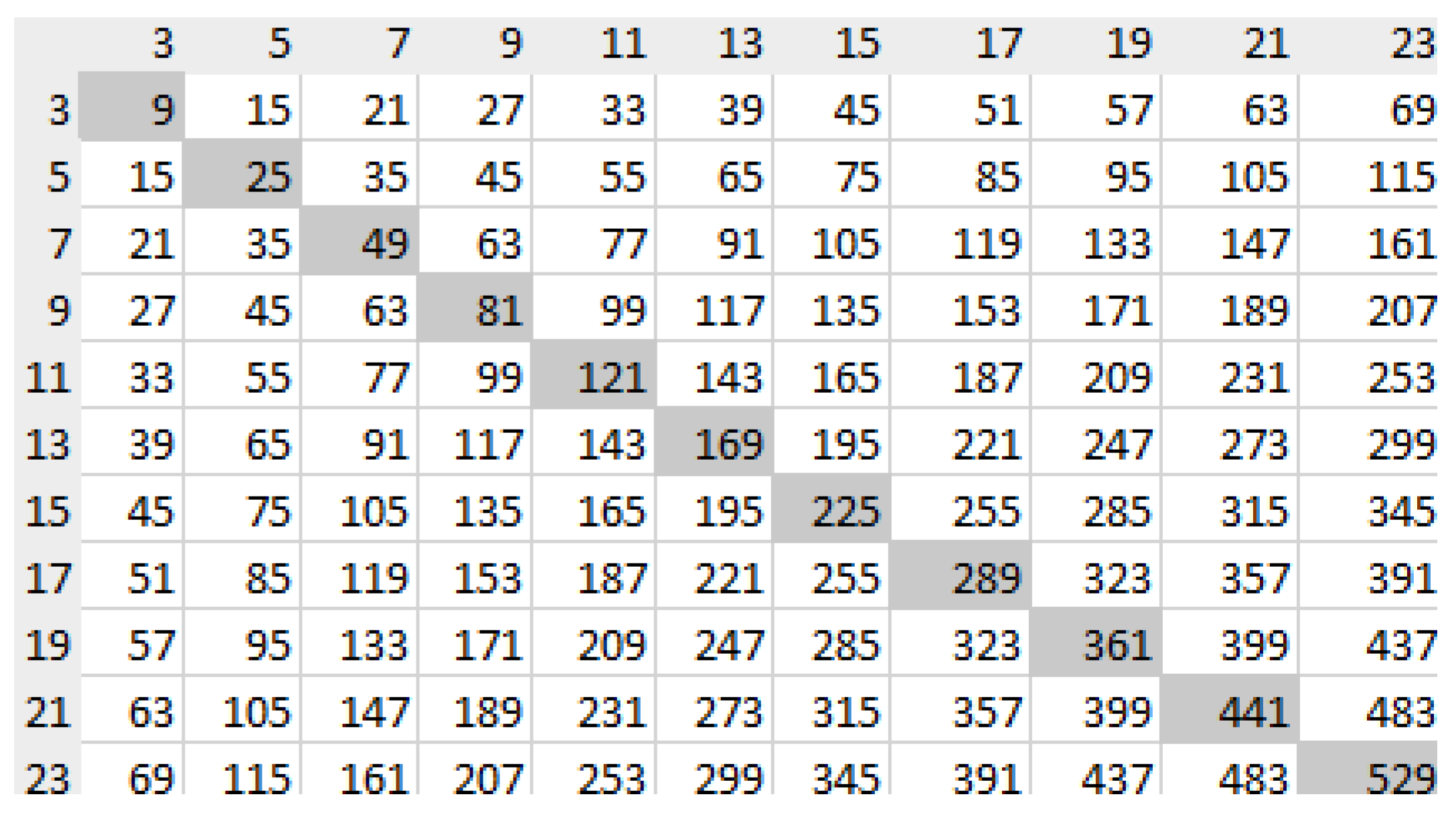
Figure 2.
Variation in the count of odd numbers during the elimination of composite numbers, calculated according to the pseudocode for (these variations are accumulated in the list, see lines (3) and (8) in pseudocode).
Figure 2.
Variation in the count of odd numbers during the elimination of composite numbers, calculated according to the pseudocode for (these variations are accumulated in the list, see lines (3) and (8) in pseudocode).
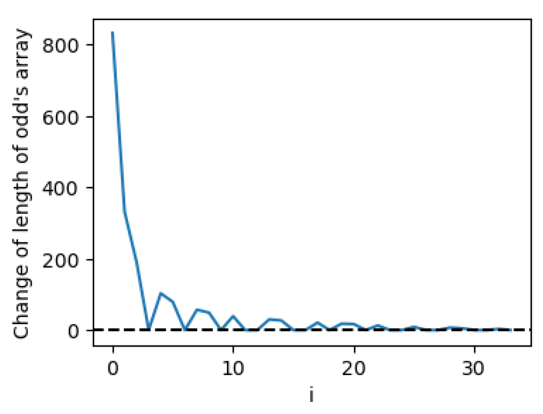
Figure 3.
The original function (blue line) of variations of odd numbers during of elimination of composite numbers (these variations are calculated according to the pseudocode and are hold in the list (lines 3 and 8 in the pseudocode)), and the function (orange line) defined as (22) for ).
Figure 3.
The original function (blue line) of variations of odd numbers during of elimination of composite numbers (these variations are calculated according to the pseudocode and are hold in the list (lines 3 and 8 in the pseudocode)), and the function (orange line) defined as (22) for ).
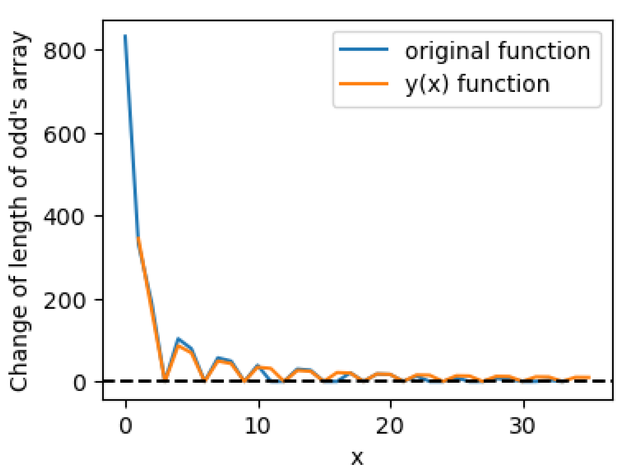
Figure 4.
The original function (blue line) of variations of odd numbers during of elimination of composite numbers (these variations are calculated according to the pseudocode and are hold in the list (line 3 and 8 in the pseudocode)), and the function (orange line) defined as (22) for (magnified image).
Disclaimer/Publisher’s Note: The statements, opinions and data contained in all publications are solely those of the individual author(s) and contributor(s) and not of MDPI and/or the editor(s). MDPI and/or the editor(s) disclaim responsibility for any injury to people or property resulting from any ideas, methods, instructions or products referred to in the content. |
© 2025 by the authors. Licensee MDPI, Basel, Switzerland. This article is an open access article distributed under the terms and conditions of the Creative Commons Attribution (CC BY) license (http://creativecommons.org/licenses/by/4.0/).
Copyright: This open access article is published under a Creative Commons CC BY 4.0 license, which permit the free download, distribution, and reuse, provided that the author and preprint are cited in any reuse.


