Submitted:
08 December 2025
Posted:
11 December 2025
You are already at the latest version
Abstract
A new philosophy of hypothesis testing - the constrained Bayesian method (CBM) and its application for testing different types of statistical hypotheses such as: simple, composite, asymmetric, multiple hypotheses, are considered in the work. The advantage of the CBM over existing classical methods is theoretically proven in the form of theorems and practi-cally demonstrated by the results of numerous example computations. Examples of the use of CBM to solve some practically important problems are presented, which confirm the flexibility of the method and its great ability to deal with difficult problems.
Keywords:
hypothesis
; constrained Bayesian method
; simple
; composite and multiple hypotheses
; parallel methods
; sequential methods
; equi-correlation coefficient
; ANOVA
MSC: 62F15, 62F03
1. Introduction
As is known, there are four main approaches (philosophies) to statistical hypothesis testing, which differ from each other in the formalization of the problem, the metrics introduced, and the characteristics of the information used. These approaches are: Fisher’s [1], Neyman-Pearson’s [2], Jeffrey’s (so-called Bayesian) [3] (so-called parallel methods) and Wald’s (so-called sequential method) [4]. Based on these ideas, many methods have been developed and successfully used to solve various problems.
Since the late 1970s, we have been developing a new approach (philosophy) for testing hypotheses, which we have called the Constrained Bayesian Method (CBM).
As is known, two types of errors can be made when testing hypotheses: rejecting the true hypothesis (decision) and accepting the false hypothesis (decision). The measures of the possibility of making these decisions, i.e. probabilities, are called the levels of the first type (Type I) and second type (Type II) errors, respectively.
Unlike the classical Bayesian method, where an unconstrained optimization problem is solved, namely, the general loss function containing type I and type II errors is minimized, in CBM the minimization is performed of one type of error under the condition of imposing restrictions on another type of errors.
Depending on the constraints, it is possible to formulate seven different tasks, which allows us to very flexibly choose the appropriate task based on the characteristics of the problem to be solved [5]. In three of them, the levels of type I errors are limited and the levels of type II errors are minimized. In the following four, Type II error rates are limited and Type I error rates are minimized.
For clarity, let us give one formulation for each of these two groups.
2. Constrained Bayesian Method
Let us introduce the following notations: is dimensional random variable with distribution density ; , , are quantity testable hypotheses, where , ; are non-intersecting subsets ; is dimensional parameter space; is a priori probability of hypothesis; is the density of the distribution of under the fairness of hypothesis; is the area of acceptance of hypothesis; and are losses caused by wrongly accepting and wrongly rejecting hypotheses.
2.1. Restrictions on the Conditional Probabilities of Accepting True Hypotheses (CBM 2)
The average loss caused by incorrectly accepting hypotheses is minimizing
subject to
The solution of this problem gives
where the Lagrange multipliers , , are determined so that the equalities in (2) hold.
2.2. Restrictions on Posterior Probabilities of Rejecting True Hypotheses (CBM 7)
In this case, we are looking for the maximum of the average probability of accepting true hypotheses (let us call it the average power of the criterion)
at the following restrictions
Lagrange’s method gives us
where, are determined so that the equalities in (5) hold.
3. General Characterization of the CBM
CBM turned out to be a generalization of existing methodologies, which gives unique results in terms of the optimality of the obtained decisions under the conditions of the minimum number of observations. Constrained Bayesian methodology surpasses in existing methodologies in that: 1) it uses all the information that existing methodologies use; 2) at formalization, all features of formalization of existing methodologies are taken into account.
In particular, the constrained Bayesian methodology uses not only the loss function and a priori probabilities to make decisions, as the classical Bayesian methodology does, but also the significance level of the criterion, as the frequentist (Neiman-Pearson) methodology does, and it is data-dependent like the Fisher methodology. The combination of these capabilities has increased the quality of the decisions made in the Constrained Bayesian methodology compared to other methodologies.
Constrained Bayes methodology has been used to test various types of hypotheses, such as simple, composite, asymmetric, multiple hypotheses, for which the superiority of CBMs compared to existing methods has been theoretically proven in the form of theorems and practically demonstrated by the results of many example calculations [5,6]. When testing the mentioned hypotheses, the constrained Bayesian methodology allows to obtain such decision rules, which, without any coercion, naturally allow to minimize practically all existing criteria of optimality of the decision, such as: type I, II and III error rates; false acceptance rate (); pure directional false discovery rate (); mixed directional false discovery rate (); Family-wise error rates of type I and type II (, ) and others.
To illustrate what has been said, let us quote some results obtained using the mentioned methodology.
Let us define the summary risk (SR) of making an incorrect decision when testing hypotheses as a weighted sum of the probabilities of making incorrect decisions, i.e.
Here is the sum function of losses caused by both types of errors.
It is clear that for given losses and probabilities, SR depends on decision areas. Let us note: and are the regions of acceptance of hypotheses, respectively, in constrained Bayesian (CBM) and Bayesian (B) methods; and are, respectively, the summary risks (SR) in constrained Bayesian and Bayesian methods.
Theorem 1.
For given losses and probabilities, SR of making incorrect decision in CBM is a convex function of
with a maximum at . By increasing or decreasing , SR decreases, and in the limit, i.e., at or , SR tends to zero.
From the theorem directly follows the following.
Corollary 1.
At the same conditions SR of making the incorrect decision in CBM is less or equal to SR of the Bayesian decision rule, i.e., .
Similar to Corollary 1, it is not difficult to be convinced that SR of making an incorrect decision in the CBM does not exceed the SR of the frequentist method, that is, , where is the SR of the frequentist method.
The following theorem is equitable [8].
Theorem 2.
Let us assume that probability distributions , , are such that, at increasing number of repeated observations , the entropy concerning distribution parameter , in relation to which the hypotheses are formulated, decrease. In such a case, for all given values and there can always be found such a finite, positive integer number that inequalities and , where the number of repeated observations is , take place.
Here and are the probabilities of errors of the first and the second types, respectively, in constrained Bayesian task when the decision is made on the basis of arithmetic mean of the observation results calculated by repeated observations. That is, the CBM allows us to make a decision by increasing information so that the levels of possible first and second type errors are restricted to any desired level.
Let us bring examples of the use of the CBM in cases of different types of hypotheses (simple, composite, asymmetric, multiple) and show its advantage over existing methods.
4. Simple Hypotheses
4.1. Parallel Methods
Example 1 [9]. Suppose that are independent identically distributed (i.i.d.) random variables with distribution law . Let us test the basic hypothesis against the alternative .
Below, when discussing examples, we assume that the hypotheses are a priori equally probable.
Table 1 presents the results of testing hypotheses using various criteria for various calculated from observations.
The results of the computation show that the Berger ( and criteria), Bayesian, and Neyman-Pearson methods accept the alternative hypothesis on the basis of , i.e. , when there is no basis for such a decision [9]. Both hypotheses are equally likely to be true or false.
In this respect, Fisher’s -value test is better because it rejects the hypothesis but says nothing about . However, the probability value does not provide any information about the existence of another possible hypothesis instead of . In this situation, CBM gives the most logical answer, because it confirms that both hypotheses are equally true or equally false, that is, an unambiguous decision cannot be made in this case. For other values of the statistic , all the considered methods make correct decisions with different error probabilities. But even in these cases, the advantage of CBM is obvious, because it gives us the error levels of Type I and Type II for which one of the testable hypotheses can be accepted according to the given statistic .
4.2. Sequential Methods
Example 2 [9]. Let us consider the scenario of Example 1, but assume that the data is obtained sequentially.
The results of the computation of 17 random samples generated by sequentially processed are given in Table 2, where the arithmetic mean of the observations is indicated by .
4.3. Sequential Methods
Example 3 [9]. Let us consider the scenario of Example 1, but assume that the data is obtained sequentially.
The results of the computation of 17 random samples generated by sequentially processed are given in Table 3, where the arithmetic mean of the observations is indicated by .
The table shows that the Wald and Berger tests give the same results, although the error probabilities in the Berger test are slightly lower than in the Wald test due to the fact that Berger calculated the error probabilities with a given value of the statistic. In the Wald criterion, they are determined by the decision thresholds. Out of 17 observations, correct decisions were made 7 times based on 3, 3, 5, 1, 1, 3, and 1 observations in both tests, and all decisions were correct. The average number of observations in making a decision is equal to 2.43. With the Bayesian-type sequential method, correct decisions for the same sample were made 10 times based on 1, 2, 2, 1, 3, 2, 1, 1, 3, and 1 observations, and all decisions were also correct. The average number of observations in making a decision is equal to 1.7.
5. Composite Hypotheses
Similar to the cases above, where CBM is optimal for testing simple hypotheses in parallel and sequential experiments, it retains optimal properties when testing composite hypotheses. Also, it easily, without much effort, overcomes Lindley’s paradox, which arises when testing a simple hypothesis against a composite hypothesis. These facts are shown theoretically and based on the computation of specific examples in the work [10].
6. Testing Multiple Hypotheses
For several last decades, multiple hypotheses testing problems have attracted significant attention because of their huge applications in many fields (see, for example, [11–17 and so on]).
CBM maintains optimal properties when testing multiple hypotheses. For example, in [18] were considered individual hypotheses about parameters of sequentially observed vectors
The following stopping rule in the sequential test was developed
where and are Lagrange multipliers obtained in CBM; is the likelihood ratio (10) for the th parameter () calculated on the basis of sequentially obtained observation results
The following theorem was proved [18]
Theorem 3. A sequential Bonferroni procedure for testing multiple hypotheses (8) with stopping rule (9), rejection regions , and acceptance regions , where and are defined in CBM for and , controls both error rates at levels and .
The computed results (given in [18]) clearly demonstrate the validity and optimality of the developed scheme in comparison with the existing methods.
7. Testing Multiple Hypotheses with Directional Alternatives in Sequential Experiments
Testing a simple basic hypothesis versus composite alternative is a common, well-studied problem in many scientific works [19,20,21,22,23,24,25,26]. In many problems, whether to make a decision in favor of the alternative hypothesis as well as making sense of the direction of difference between parameter values, defined by basic and alternative hypotheses, is important; that is, making a decision whether the parameter outstrips or falls behind the value defined by the basic hypothesis is meaningful [27,28,29,30,31,32,33]. Such problems occur, for example, in microarray data analysis, imaging analysis, biological applications and genetic research [32,34] and many others.
For parametrical models, this problem can be stated as
where is the parameter of the model, is known. These alternatives are called skewed or directional alternatives.
In many applications, the case of multiple directional hypotheses is considered, i.e. the testing hypotheses are the following [29,31,33,34,35]
where is the number of individual hypotheses about parameters that must be tested by test statistics , where .
The following theorem for hypotheses (11) is proved in [36].
Theorem 4.
Let us assume that the probability distributions
, , where , are such that, at increasing number of observations in the sample, the entropy concerning distribution parameter , in relation to which the hypotheses are formulated, decreases. In such case, for given set of hypotheses , and , there always exists such sample of size on the basis of which decision concerning tested hypotheses can be made with given reliability when Lagrange multipliers are determined for in decision making regions and the condition is satisfied.
For multiple directional hypotheses (12) the stopping rule is as follows:
where , , are independent -dimensional observation vectors with correlated parameters; is -th hypothesis acceptance region for -th sub-set of hypothesis.
The following theorem is proved in [36].
Theorem 5.
Let’s for each sub-set of directional hypotheses of multiple hypotheses (12) one of the possible stated task of CBM is used with the restriction levels providing the condition
, . Then, if , , are taken so that , the following condition is fulfilled.
Here is the total mixed directional false discovery rate that was introduced in [36].
8. Testing Composite Hypotheses Concerning Normal Distribution with Equal Parameters
In a large variety of practical situations, a normal distribution with equal parameters, that is , may be postulated as a useful model for data [37,38,39].
Let us consider a random variable distributed as . The problem is to test the hypotheses
on the basis of independent identically distributed (i.i.d.) random variables .
The following theorems for directional alternatives were proved in [36].
Theorem 6.
CBM 7, at satisfying a condition
(i.e. ), where , , ensures a decision rule with (i.e. with ) less or equal to , i.e. with the condition .
Theorem 7.
CBM 7, at satisfying a condition
(i.e. ), where , , ensures a decision rule with less or equal to , i.e. with the condition .
Here, we have: as the false acceptance rate; , , are restriction levels in CBM 7; is the loss for incorrect acceptance of hypothesis.
Moreover, the following theorems are proven in [39].
Theorem 8.
CBM 2, for hypotheses (12), ensures a decision rule with the error rates of the Type-I and Type-II restricted by the following inequalities
Theorem 9.
CBM 2, for hypotheses (12), ensures a decision rule with the averaged loss of incorrectly accepted hypotheses and
the averaged loss of incorrectly rejected hypotheses restricted by the following inequalities
Correctness of these theorems and superiority of CBM over Bayes method are clearly demonstrated by computation results.
9. Testing Equi-Correlation Coefficient
Symmetric Multivariate Normal Distribution (SMND) is widely used in many applications of different spheres of human activities such as psychology, education, genetics and so on [40]. It is also used extensively in statistical inference procedures, e.g., in analysis of variance (ANOVA) for modeling of the error part [41].
Let the -dimensional random vector follow the -variate normal distribution with zero mean vector and correlation matrix of the following structure:
where is an identity matrix and is matrix of ones.
The support of , assures the non-singularity of the correlation matrix [41].
The problem, we want to solve, can be formulated as follows: to test
on the basis of the sample . Here is the Helmert orthogonal transformation on uncorrelated multivariate normal vectors sequence , i.e. where is the Helmert matrix given as [41]
i.e. is -dimensional random vector with independent components each of which has zero mean and variances determined by
The probability density function (pdf) of is
To test hypotheses (17) were applied CBM using the maximum likelihood estimation and Stein’s approach [43]. Simulation results showed that CBM using Stein’s approach gives opportunities to make decisions with higher reliability for testing (17) hypotheses then Bayes method (see Figure 1).
The samples for making decisions are generated by (21) with for the size .
10. Solving ANOVA Problem with Restricted Type I and Type II Error Rates
The problem of comparing the means of several normally distributed random variables attracted researchers’ attention from the middle of last century. Such problems arise in many practical applications. For example, at comparing treatment effects in clinical trials, or experimental studies at comparing effects of different experiments, or at comparing the failure rate of a machine with its ages [44]. Also, an important question in many applications is whether the nonparametric time trends are all the same [45]. In the framework of ANOVA, the problem can be formulated as follows [46]. Let’s consider normal populations , . Let be a random sample from , independent from each other. The problem is to test hypotheses
In some studies the researcher may believe before observing the data that the true means are simply ordered (). For example, the treatment means may be a sequences of increasing dose levels of a drug. In this case ANOVA takes the form
with at least one strict inequality. This statement has received considerable attention in the statistical literature (see, for example, [46,47,48,49,50]).
The simplest case , i.e. the case with only two normal populations, called as the Behrens-Fisher problem, is well studied. For its solution, at the statement (23), a simple and accurate method is introduced in [51,52] which gives good results in both cases when variances are equal or are not. For arbitrary case, when a compact but quite good review of the existed methods of solving the problem (23) is given in [53], on the basis of which there is concluded that a procedure that gives satisfactory results by Type I error rate for all sample sizes, large and parameters configurations does not exist [53,54].
For the statement (24), a one-sided studentized range test is offered in Hayter [48]. It provides simultaneous one-sided lower confidence bounds for the ordered pairwise comparisons ,. Similar inference procedures are discussed in many works.
Without loss of generality, we can suppose that all () are positive, because if this condition is not fulfilled, we can always achieve it by moving the origin.
Let us rewrite hypotheses (23) as follows
where , . In this case, hypotheses (24) take the form
vs. , with at least one strict inequality, (26)
Using the concept of directional hypotheses [5], hypotheses (25) can be considered as a set of directional hypotheses
vs. or , . (27)
Statement (27) allows us to test hypotheses (23) and (24) (which are the same as hypotheses (25) and (26)) simultaneously, using techniques developed in [6,36]. In particular: after testing hypotheses (27), if for even one value of , left sided hypothesis is accepted among accepted alternatives, accept alternative hypothesis in (25), if all the accepted alternative hypotheses are right sided – accept alternative hypothesis in (26), otherwise accept the null hypothesis.
To test a subset of individual hypotheses of (27) the following hypothesis was proven.
Theorem 10.
CBM 7, at satisfying a condition
, where , ensures a decision rule with Type I error rate less or equal to , i.e. with the condition .
For testing multiple directional hypotheses (27), the concept of the was used
To provide a level for the total Type I error rate () and for the total Type II error rate (), we provide , the level of the appropriate criteria for the th subset of the individual directional hypotheses. As a result, we have
where and are the Type I error rate and the Type II error rate, respectively, of the th subset of directional hypotheses [18,36].
The values of in all three cases (for , for and for ) can be chosen to be equal, i.e. or different, e.g. inversely proportional to the informational distances between the tested hypotheses in the subsets of directional hypotheses [36].
The offered method of solving ANOVA problem, for known and unknown variances of observation results, with restricted Type I and Type II error rates based on CBM gives very reliable results that surpass the existing methods for today. The latter is confirmed by the calculation results of practical examples by simulating different scenarios [44].
The offered method is a sequential one that requires a set of observations to make a decision.
11. Conclusion
A brief review of the application of CBM to test different types of statistical hypotheses arising in many practical problems are considered above. It confirms the advantage of the CBM over existing classical methods at testing simple, composite, asymmetric, multiple hypotheses of different kinds. Obtained results, published in many important scientific publication, confirm the flexibility of the method and its great ability to deal with difficult problems.
Author Contributions
Conceptualization, Kartlos Kachiashvili; methodology, Kartlos Kachiashvili; software, Joseph Kachiashvili; validation, Kartlos Kachiashvili, Joseph Kachiashvili; formal analysis, Kartlos Kachiashvili, Joseph Kachiashvili; investigation, Kartlos Kachiashvili, Joseph Kachiashvili;; resources, Kartlos Kachiashvili, Joseph Kachiashvili; data curation, Joseph Kachiashvili; writing—original draft preparation, Kartlos Kachiashvili; writing—review and editing, Kartlos Kachiashvili, Joseph Kachiashvili; visualization, Joseph Kachiashvili; supervision, Kartlos Kachiashvili; project administration, Kartlos Kachiashvili; funding acquisition, Joseph Kachiashvili All authors have read and agreed to the published version of the manuscript.
Funding
The research of the second author [PHDF-25-1783] has been supported by the Shota Rustaveli National Science Foundation of Georgia (SRNSFG).
Data Availability Statement
The data on which the computation results were obtained in the article were generated by the authors, as described in the relevant publications cited in the paper.
Conflicts of Interest
The authors declare no conflicts of interest.
Abbreviations
The following abbreviations are used in this manuscript:
| CBM | Constrained Bayesian method |
| FAR | False acceptance rate |
| pdFAR | Pure directional false discovery rate |
| mdFAR | Mixed directional false discovery rate |
| FWERI | Family-wise error rates of type I |
| FWERII | Family-wise error rates of type II |
| SR | Summary risk |
| tmdFAR | Total mixed directional false discovery rate |
| i.i.d. | Independent identically distributed |
| SMND | Symmetric Multivariate Normal Distribution |
| ANOVA | Analysis of variance |
| TTIER | Total Type I error rate |
| TTIIER | Total Type II error rate |
References
- Fisher R.A. Statistical Methods for Research Workers, London: Oliver and Boyd, 1925.
- Neyman J.; Pearson E. On the Problem of the Most Efficient Tests of Statistical Hypotheses, Philos. Trans. Roy. Soc., Ser. A, 1933; Volume 231, pp. 289-337.
- Jeffreys H. Theory of Probability, 1st ed. Oxford: The Clarendon Press, 1939.
- Wald A. Sequential analysis, New-York: Wiley, 1947a.
- Kachiashvili K.J. Constrained Bayesian Methods of Hypotheses Testing: A New Philosophy of Hypotheses Testing in Parallel and Sequential Experiments. Nova Science Publishers, Inc., New York, 2018; pp. 361.
- Kachiashvili K.J. Testing Statistical Hypotheses with Given Reliability, Cambridge Scholars Publishing, UK, 2023; pp. 322.
- Kachiashvili K.J.; Bansal N.K.; Prangishvili I.A. Constrained Bayesian Method for Testing the Directional Hypotheses. Journal of Mathematics and System Science 2018, Volume 8, 96-118.
- Kachiashvili K.J.; Mueed A. Conditional Bayesian task of testing many hypotheses. Statistics 2013, Volume 47(2), 274-293.
- Kachiashvili K.J. Comparison of Some Methods of Testing Statistical Hypotheses. International Journal of Statistics in Medical Research 2014, Volume 3, 174-189.
- Kachiashvili K.J. Constrained Bayesian Method of Composite Hypotheses Testing: Singularities and Capabilities. International Journal of Statistics in Medical Research 2016, Volume 5(3), 135-167.
- O’Brien, P.C. Procedures for Comparing Samples with Multiple Endpoints, Biometrics 1984, Volume 40, 1079–1087.
- Pocock, S.J.; Geller, N.L.; Tsiatis, A.A. The Analysis of Multiple Endpoints in Clinical Trials, Biometrics 1987, Volume 43, 487–498.
- Shaffer, J.P. Multiple Hypothesis Testing, Annual Review of Psychology 1995, Volume 46, 561-584.
- Dudoit, S.; Shaffer, J.P.; Boldrick, J.C. Multiple Hypothesis Testing in Microarray Experiment, Statistical Science 2003, Volume 18, 71–103.
- Tartakovsky, A.G.; Veeravalli, V.V. Change-Point Detection in Multichannel and Distributed Systems with Applications. In Applications of Sequential Methodologies, Mukhopadhyay N., Datta S., Chattopadhyay S. Dekker: New York, 2004; pp. 339–370.
- De, S.K.; Baron, M. Step-up and Step-down Methods for Testing Multiple Hypotheses in Sequential Experiments. Journal of Statistical Planning and Inference 2012a, Volume 142, 2059–2070.
- De, S.K.; Baron, M. Sequential Bonferroni Methods for Multiple Hypothesis Testing with Strong Control of Family-Wise Error Rates I and II. Sequential Analysis 2012b, Volume 31, 238–262.
- Kachiashvili K.J. Constrained Bayesian Method for Testing Multiple Hypotheses in Sequential Experiments. Sequential Analysis, Design Methods and Applications 2015, Volume 34(2), 171-186.
- Wijsman, R.A. Cross-Sections of Orbits and Their Application to Densities of Maximal Invariants. In Proceedings of the Fifth Berkeley Symposium on Mathematical Statistics and Probability, Lucien M. Le Cam and Jerzy Neyman, eds., University of California, Oakland, 1967, pp. 389–400.
- Anderson, S. Distributions of Maximal Invariants Using Quotient Measures. Annals of Statistics 1982, Volume 10, 955–961.
- Berger, J.O.; Pericchi L.R. The Intrinsic Bayes Factor for Model Selection and Prediction. Journal of American Statistical Association 1996, Volume 91, 109–122. [CrossRef]
- Kass, R.E.; Wasserman, L. The Selection of Prior Distributions by Formal Rules. Journal of American Statistical Association 1996, Volume 91, 1343–1370. oi:10.1080/01621459.1996.10477003.
- Marden, J. I. Hypothesis Testing: From p Values to Bayes Factors. Journal of American Statistical Association 2000, Volume 95, 1316–1320. [CrossRef]
- Gomez-Villegas, M. A.; Main, P.; Sanz, L. A Bayesian Analysis for the Multivariate Point Null Testing Problem, Statistics 2009, Volume 43, 379–391. [CrossRef]
- Bedbur, S.; Beutner, E.; Kamps, U. Multivariate Testing and Model-Checking for Generalized Order Statistics with Applications. Statistics 2013, Volume 48, 1–114. [CrossRef]
- Duchesne, P.; Francq, Ch. Multivariate Hypothesis Testing Using Generalized and {2}-Inverses-With Applications. Statistics 2014, Volume 49, 1–22. [CrossRef]
- Kaiser, H.F. Directional Statistical Decisions, Psychological Review 1960, Volume 67, 160–167. [CrossRef]
- Leventhal, L.; Huynh, C. Directional Decisions for Two-Tailed Tests: Power, Error Rates, and Sample Size. Psychological Methods 1996, Volume 1, 278–292. [CrossRef]
- Finner, H. Stepwise Multiple Test Procedures and Control of Directional Errors, Annals of Statistics 1999, Volume 27, 274–289. [CrossRef]
- Jones, L.V.; Tukey, J.W. A Sensible Formulation of the Significance Test, Psychological Methods 2000, Volume 5, 411–414. [CrossRef]
- Shaffer, J.P. Multiplicity, Directional (Type III) Errors, and the Null Hypothesis, Psychological Methods 2002, Volume 7, 356–369. [CrossRef]
- Bansal, N.K.; Sheng, R. Bayesian Decision Theoretic Approach to Hypothesis Problems with Skewed Alternatives. Journal of Statistical Planning and Inference 2010, Volume 140, 2894-2903. [CrossRef]
- Bansal, N. K.; Hamedani, G. G.; Maadooliat, M. Testing Multiple Hypotheses with Skewed Alternatives. Biometrics 2016, Volume 72, 494–502.
- Bansal, N.K; Miescke, K. J. A Bayesian Decision Theoretic Approach to Directional Multiple Hypotheses Problems. Journal of Multivariate Analysis 2013, Volume 120, 205–215. [CrossRef]
- Benjamini, Y.; Hochberg, Y. Controlling the False Discovery Rate: A Practical and Powerful Approach to Multiple Testing. Journal of the Royal Statistical Society - Series B 1995, Volume 57, 289–300. [CrossRef]
- Kachiashvili K.J.; Kachiashvili J.K.; Prangishvili I.A. CBM for Testing Multiple Hypotheses with Directional Alternatives in Sequential Experiments. Sequential Analysis 2020, Volume 39(1), 115-131. [CrossRef]
- Mukhopadhyay N,; Zhang, C. EDA on the Asymptotic Normality of the Standardized Sequential Stopping Times, Part-I: Parametric Models. Sequential Analysis 2018, Volume 37, 342-374.
- Mukhopadhyay N.; Zhang, C. EDA on the Asymptotic Normality of the Standardized Sequential Stopping Times, Part-II: Distribution-Free Models. Sequential Analysis 2020, Volume 39, 367-398.
- Kachiashvili, K.J.; Mukhopadhyay, N.; Kachiashvili, J.K. Constrained Bayesian method for testing composite hypotheses concerning normal distribution with equal parameters. Sequential Analysis 2024, Volume 43(2), 147-178.
- SenGupta, A. On Tests for Equi-correlation Coefficient of a Standard Symmetric Multivariate Normal Distribution. Austral. J. Statist. 1987, Volume 29(1), 49-59.
- De, Sh.K.; Mukhopadhyay, N. Two-stage fixed-width and bounded-width confidence interval estimation methodologies for the common correlation in an equi-correlated multivariate normal distribution. Sequential Analysis 2019, Volume 38, 214-258. [CrossRef]
- SenGupta, A.; Gokhale, D.V. Optimal Tests for the Correlation Coefficient in a Symmetric Multivariate Normal Population. Journal of Statistical Planning & Inference 1986, Volume 14, 256-263.
- Kachiashvili, K.J.; SenGupta, A. Constrained Bayesian Method for Testing Equi-Correlation Coefficient. Axioms 2024, Volume 13(10), 722. [CrossRef]
- Kachiashvili, K.J.; Kachiashvili, J.K.; SenGupta, A. Solving ANOVA problem with restricted Type I and Type II error rates. AIMS Mathematics 2025, Volume 10(2), 2347-2374. [CrossRef]
- Khismatullina M.; Vogt M. Multiscale Comparison of Nonparametric Trend Curves. arXiv 2022, Papers 2209.10841, arXiv.org.
- Aghamohammadi A.; Meshkani, M.R.; Mohammadzadeh M. A Bayesian Approach to Successive Comparisons. Journal of Data Science 2010, Volume 8, 541-553. [CrossRef]
- Barlow R.E.; Bartholomew D.J.; Bremner J.M.; Brunk H.D. Statistical Inference under Order Restrictions, J. Wiley & Sons Ltd., 1972; ISBN 10: 0471049700, 9780471049708.
- Hayter A.J. An one-sided studentized range test for testing against a simple ordered alternative, Journal of the American Statistical Association 1990, Volume 85, 778-785. [CrossRef]
- Ichiba S. An alternative Method for Ordered ANOVA Under Unequal Variances. Thesis of the Degree of Bachelor of Arts with Honours in Mathematics and Statistics. Acadia University, 2016. https://books.google.ge/books?id=9ipZtAEACAAJ.
- Robertson T.; Wright F.T.; Dykstra R.L. Order Restricted Statistical Inference, Wiley Series in Probability and Mathematical Statistics, John Wiley and Sons, Chichester, 1988, pp. 488. [CrossRef]
- Welch B.L. The generalization of Student’s problem when several different population variances are involved. Biometrika 1947, Volume 34, 28-35. [CrossRef]
- Welch B.L. On the comparison of several mean values: an alternative approach. Biometrika 1951, Volume 38, 330-336. [CrossRef]
- Krishnamoorthy K.; Lu F.; Mathew Th. A parametric bootstrap approach for ANOVA with unequal variances: Fixed and random models. Computational Statistics & Data Analysis 2007, Volume 51, 5731-5742. [CrossRef]
- Dajani A.N. Contributions to statistical inference for some fixed and random models, Ph.D. Dissertation. Department of Mathematics and Statistics, Baltimore County: University of Maryland, 2002.
Figure 1.
Dependence of true Hypothesis acceptance probability on correlation coefficient.
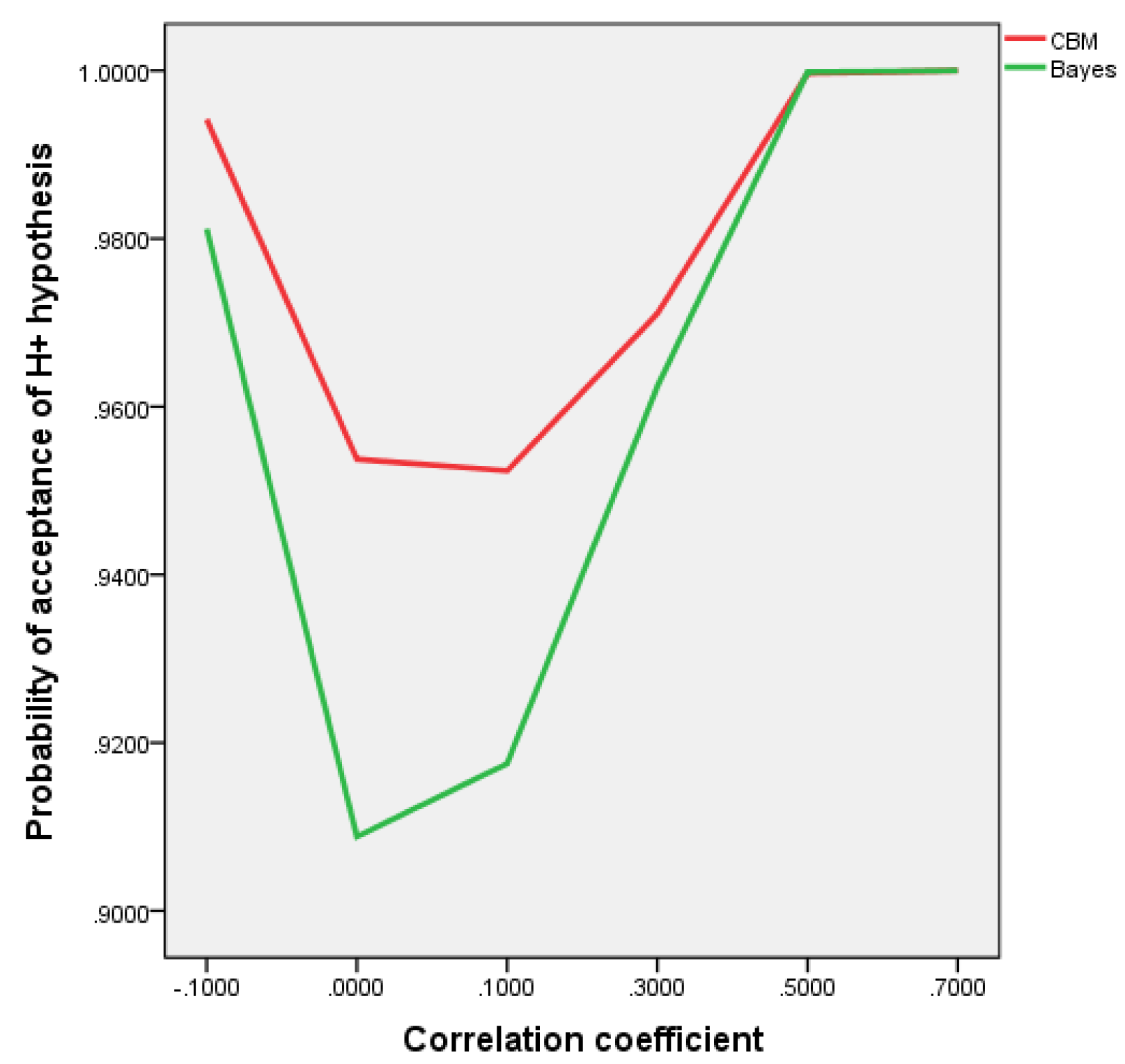

Table 1.
Results of hypothesis testing for different values of .
| For tests , and Bayes | For N-P test | For p-value test |
For constrained Bayes test (CBM) | ||||||||||
| CEP | CEP | AH*) | AH*) | -value | AH*) | AH*) | |||||||
| 0 | 1 | 0.5 | 0.5 | 0.02275 | 0.02275 | 0.02275 | Reject |
|
|
|
No one1) Bothe2) |
||
| 0.028 | 0.8 | 0.444(4) | 0.555(5) | 0.02275 | 0.02275 | 0.01989 | Reject |
|
|
|
Bothe No one |
||
| 0.25 | 0.14 | 0.1228 | 0.8772 | 0.02275 | 0.02275 | 0.00621 | Reject |
|
|
|
Bothe No one |
||
| 1 | 0.00034 | 0.00034 | 0.99966 | 0.02275 | 0.02275 | 0.00003 | Reject |
|
|
|
Bothe |
||
| -0.25 | 7.389 | 0.88 | 0.1192 | 0.02275 | 0.02275 | 0.06681 | Accept |
|
|
|
Bothe No one |
||
| -1 | 2980.958 | 0.99966 | 0.00034 | 0.02275 | 0.02275 | 0.5 | Accept |
|
|
|
Bothe |
||
*)Accepted hypothesis 1) Both hypotheses are equally impossible to be true. 2) Both hypotheses are equally likely to be true.
Table 2.
Results of hypothesis testing for normal sampling.
| Observation results |
|
The Berger’s test | The Wald’s test |
for sequential test of Bayesian type |
The sequential teat of Bayesian type | |
| 1 2 3 4 5 6 7 8 9 10 11 12 13 14 15 16 17 |
1.201596 0.043484 0.658932 0.039022 0.616960 2.026540 -0.422764 0.562569 0.353047 -0.123311 1.126263 1.521061 1.486411 -0.578935 0.623006 1.616669 1.754413 |
|
, , . , , . , , . , , . , , . , , . , , . |
|
|
|
| 2.43 | 2.43 | 1.7 |
Table 3.
Results of hypothesis testing for normal sampling.
| Observation results |
|
The Berger’s test | The Wald’s test |
for sequential test of Bayesian type |
The sequential teat of Bayesian type | |
| 1 2 3 4 5 6 7 8 9 10 11 12 13 14 15 16 17 |
1.201596 0.043484 0.658932 0.039022 0.616960 2.026540 -0.422764 0.562569 0.353047 -0.123311 1.126263 1.521061 1.486411 -0.578935 0.623006 1.616669 1.754413 |
|
, , . , , . , , . , , . , , . , , . , , . |
|
|
|
| 2.43 | 2.43 | 1.7 |
Disclaimer/Publisher’s Note: The statements, opinions and data contained in all publications are solely those of the individual author(s) and contributor(s) and not of MDPI and/or the editor(s). MDPI and/or the editor(s) disclaim responsibility for any injury to people or property resulting from any ideas, methods, instructions or products referred to in the content. |
© 2025 by the authors. Licensee MDPI, Basel, Switzerland. This article is an open access article distributed under the terms and conditions of the Creative Commons Attribution (CC BY) license (http://creativecommons.org/licenses/by/4.0/).
Copyright: This open access article is published under a Creative Commons CC BY 4.0 license, which permit the free download, distribution, and reuse, provided that the author and preprint are cited in any reuse.


