Submitted:
08 December 2025
Posted:
09 December 2025
You are already at the latest version
Abstract
We evaluated the impact of traditional versus catchment-oriented forest harvest scheduling of radiata pine plantations on profitability and rainfall-induced landslide susceptibility in the Uawa catchment, Aotearoa|New Zealand. Our hypothetical case study assumed that 59% of the Uawa catchment area is covered with radiata pine plantations (31,899 hectares). These plantations are located within 89 Catchment Management Units (CMUs) and 1123 hillslope units (HSUs). The HSUs are assumed to be the forest stands with stand ages as measured in 2024. We maximised the Net Present Value of the forests (NPV) subject to non-declining yield (NDY) constraints, considering different maximum harvesting levels (MHL) (10 to 50% of CMU area) that could be allowed for any single CMU during any single 5-year period. We found that profitability increased rapidly when the MHL increased from 10 to 20%, with only marginal increases after 25%. We calculated a proxy for rainfall-induced landslide (RIL) susceptibility as the aggregated sum of the area harvested from each HSU, multiplied by its RIL susceptibility. We then imposed constraints for our RIL proxy to become constant over successive periods. Our final catchment-oriented harvest schedule marginally reduced the Internal Rate of Return from the business-as-usual scenario, from 8.92% to 8.52%. Forest owners’ concerns about the economic and operational effects of catchment-oriented harvest scheduling appear to be surmountable.
Keywords:
catchment-oriented harvest schedule
; radiata pine plantations
; non-declining yield
; profitability
; rainfall-induced landslide susceptibility
1. Introduction
In Aotearoa|New Zealand (henceforth “New Zealand”), 24% of plantation forests are located on steep, erosion-susceptible lands (Te Uru Rākau, 2025). In many cases, these steepland plantations were deliberately established to control soil erosion that followed the large-scale clearance of indigenous forests and their conversion to grassland for pastoral farming. This strategy has proved successful. (Figure 1).
However, New Zealand’s plantation forests are usually clear-felled for commercial wood production when mature, and the steepland plantations are no exception. Clearfelling on erosion-susceptible lands results in a “window of vulnerability” (WoV), where the reinforcement of the soil by tree roots, as well as the interception of rainfall and evapotranspiration, are drastically reduced. This results in the erosion susceptibility of the clearfelled land increasing by a factor of three to ten-fold compared with land under a mature forest (Phillips et al., 2024). The WoV lasts around six years, until the replanted trees grow large enough to protect the soil (Phillips et al., 2024). Over 90% of the forest plantation area in New Zealand comprises even-aged, single-species stands of Pinus radiata D.Don (radiata pine) managed under a clearfell regime with a rotation length of approximately 28 years (Paul & Wakelin, 2024). Thus, the first six years (or 21%) of a 28-year radiata pine plantation rotation are in the WoV.
Many of the forests established for erosion control in New Zealand were planted over large areas in a short time, with entire catchments planted within three to five years in some cases. Because these plantation forests were managed as commercial forests for wood production, they were typically clearfelled at or near the average New Zealand rotation age of 28 years. This has resulted in very large clearfelling areas (Figure 2) extending for several hundreds or even thousands of hectares (Bloomberg & Urlich, 2025).
At the same time, erosion-susceptible lands in New Zealand are prone to multiple-occurrence regional landslide events (MORLEs) (Crozier, 2017). In a MORLE, large numbers of shallow landslides occur within defined areas, ranging from tens to thousands of square kilometres. In New Zealand, MORLEs are typically triggered by intense or long-duration rainfalls occurring at a regional or sub-regional scale. If a harvested forest in the window of vulnerability is subjected to a MORLE, the increased erosion susceptibility resulting from clearfell harvesting can result in much higher rates of landsliding. Because the landslide discharges are occurring on harvested sites, considerable volumes of woody debris (“slash”) are mixed in with the landslide, resulting in downstream discharges of sediment and woody material (Amishev et al., 2013).
Over the last 15 years in New Zealand, plantation forest harvesting has led to multiple sediment and logging slash impacts on downstream communities and environments (Bloomberg & Urlich, 2025). Two notable examples are:
- In June 2018, two storm events in Tairāwhiti|Gisborne District resulted in catastrophic discharges of sediment and slash from recently clearfelled plantation forests. These unauthorised discharges led to five forestry companies being prosecuted and convicted under New Zealand’s Resource Management Act 1991 (Bloomberg & Urlich 2025).
- Between 11th to 17th February 2023, Tropical Cyclone Gabrielle impacted about 40% of the North Island of New Zealand (46,000 km2). Rainfall recurrence intervals from the event varied spatially but exceeded 250 years in places (Massey et al. 2025). Massey et al. (2025) analysed landslides that occurred in the Tairāwhiti|Gisborne and Hawke’s Bay regions since these were two of the main regions affected by landslides triggered by Cyclone Gabrielle. Results showed that landslides within plantation forests preferentially occurred on slopes that had been clearfelled 3-5 years before Cyclone Gabrielle, i.e. within the WoV.
In the aftermath of Cyclone Gabrielle, a “Ministerial Inquiry into Land Use causing woody debris and sediment-related damage in Tairāwhiti and Wairoa” (MILU) was convened (Ministry for the Environment (MfE), 2023). The MILU recognised the link between clearfelling and landsliding on erosion-susceptible land. It recommended a halt to large-scale clearfell harvesting in Tairāwhiti|Gisborne and the neighbouring Wairoa District, with maximum coupe sizes of 40 ha and limits to the annual clearfelled area within a catchment of ≤5% per year (Ministry for the Environment (MfE), 2023).
Internationally, such “catchment-oriented harvesting” (restrictions on the size and location of clearfell coupes) is a widely accepted strategy (Bloomberg et al., 2019). In contrast, the need for small clearfelling coupes has not been accepted unconditionally by the New Zealand forest industry (Bloomberg & Urlich, 2025). However, objections to small clearfelling coupes are hypothetical, since there are few examples in New Zealand where large single-age plantation forests have been systematically harvested with coupe size and location restrictions.
Therefore, the aim of this study was to assess the impact of traditional versus catchment-oriented harvest schedules on financial returns, wood flows, rainfall-induced landslide (RIL) susceptibility and the location and size of areas in the WoV. Specifically, we aimed to test the hypothesis that a catchment-oriented approach to harvest scheduling can mitigate susceptibility to rainfall-induced landslides with minimal impact on the economic performance of forests. We predict that some of the alleged drawbacks of catchment-oriented harvest scheduling are surmountable.
2. Materials and Methods
2.1. Study Area
The hypothetical case study simulates the management of radiata pine plantations located in the Uawa catchment, Tairāwhiti|Gisborne district, New Zealand (Figure 3). This area was chosen because it was severely impacted by the June 2018 storm events, with prior clear-felling of several thousand hectares of forest over a 3- to 5-year period, leading to catastrophic effects downstream (Ministry for the Environment (MfE), 2023). Much of this clearfelled forest was replanted in radiata pine, so that large areas of even-age plantation forests will become ready for harvest from 2045 onwards. We suggest that unconstrained clearfell harvesting of these plantation forests could result in a landslide disaster of a similar scale to the June 2018 events.
The Uawa catchment has a total area of 53,866 ha and a perimeter of 168 km. Terrain varies substantially across the catchment (Figure 3c), being generally gentler in the lower part and rugged in the upper part where radiata pine plantations are mostly located. The Uawa catchment has an average slope of 32% (± 20%) while the forest plantations have an average slope of 38% (± 16%) (Table 1). Furthermore, in terms of rainfall-induced landslide (RIL) susceptibility (Figure 4), most areas are concentrated between probabilities of 0.4 and 0.6 (44%) and 0.6 and 0.8 (42%), with only 14% of the area below 0.4, and only 1.3% above 0.8. In spite that slopes between 30% and 40% are generally considered the upper operational limit for ground-based harvesting systems (Erber et al., 2025; Leitner et al., 2023; Mologni et al., 2016), the generalised high values of RIL susceptibility in the Uawa catchment suggest that, in practice, even the easier terrain would be cable harvested.
2.2. The Forestry Catchment Planner
The Forestry Catchment Planner (FCP) is a geospatial app that uses region-wide maps of plantation forest areas and ages to predict where and when clearfell harvesting is likely to occur, and therefore, forest land will be in the WoV. The FCP then uses maps of erosion susceptibility to show if the land in the WoV is highly erosion-susceptible, and therefore more likely to generate landslides and other erosion processes. This allows visualisation of the future spatial distribution of the risk of sediment (from erosion) and harvesting slash discharges (MapHQ, 2024). Currently, the FCP covers the Tairāwhiti|Gisborne District and the Hawkes Bay regions in the North Island of New Zealand, as well as the Te Tau Ihu region (comprising Nelson, Marlborough, and Tasman Districts) in the South Island of New Zealand (Figure 3a).
In this study, we use the FCP to:
- Predict the spatial and temporal occurrence of plantation forest clearfelling in the Uawa catchment over a 30-year planning period (2025-2055), under different catchment-oriented harvesting scenarios.
- Identify the landslide susceptibility of areas clearfelled under the different scenarios.
We then use the predicted plantation forest clearfelling for each scenario to calculate forest wood flows, cash flows, RIL flows and economic performance. Thus, we can evaluate each scenario using both commercial (wood flow, cash flow and economic) and environmental (landslide and erosion mitigation) criteria.
2.2.1. Catchment Management Units (CMUs)
The “Ministerial Inquiry into Land Use causing woody debris and sediment-related damage in Tairāwhiti and Wairoa” (MILU) recommended maximum coupe sizes of 40 ha and limits to the annual clearfelled area within a catchment of ≤5% of the catchment area (Ministry for the Environment (MfE), 2023). However, it did not define what a “catchment” was, so the “5%” annual area limit could not be applied to any practical situation.
To solve this problem, the FCP defines a catchment in terms of “Catchment Management Units” (CMUs), which divide the landscape into units for visualising and managing the location of clearfell harvesting in steepland forests.
CMU’s are defined using a longstanding concept in fluvial geomorphology where a fluvial system comprises three parts (Table 2): Zone 1 comprises the headwater subcatchments from which most sediment and water originate; downstream of Zone 1 is Zone 2, the transfer zone in which, if stable, sediment inputs equal sediment outputs; and downstream of Zone 2 is Zone 3, the area where deposition is the dominant process (Gellis et al., 2016).
A CMU is a subcatchment upstream from where Zone 2 transitions to Zone 1. A CMU will therefore contain Order 1 and 2 streams that flow together into an Order 3 stream. This confluence with Order 3 streams typically occurs at a “pour point” through which all sediment and water discharges flow from a Zone 1 subcatchment into a river channel located in Zone 2.
This concept works well in the New Zealand context, since most steepland plantation forests on erosion-susceptible land are located in Zone 1. Discharges of sediment and woody debris from a CMU in Zone 1 will directly impact the natural and built environment in Zone 2, although sediment and woody debris will eventually be transported by the fluvial system down to Zone 3 or even the coastline.
2.2.2. Hill Slope Units (HSU)
In the FCP, each CMU is subdivided into multiple hillslope units (HSUs) that are typically Order 1 or 2 catchments (“headwater streams”). These headwater streams are dominated by steep slopes and high stream gradients, where erosion is the dominant landscape process. We do this because, within each CMU, there can be significant variation in erosion susceptibility and landsliding. Each HSU represents areas in the landscape that are reasonably similar in erosion susceptibility and, therefore, in the likelihood that they will deliver woody debris and sediment downslope to the pour-point at the mouth of the CMU.
The average size of HSUs within the areas covered by the FCP is 28 ha (ranging from 1-450 ha). HSUs were defined using the watersheds in the New Zealand River Environments Classification (REC2) database (Snelder & Biggs, 2002). HSUs usually correspond to Order 1 and/or Order 2 subcatchments in the REC2 classification. Some REC2 watersheds occur on both sides of the stream channel. These were split using the REC2 riverlines so that individual HSUs were defined on either side of the channel. Areas of flat land on floodplains, terraces or low fans were removed from the hillslope units. These flat lands were identified using data from the New Zealand Land Resource Inventory database (MWLR, 2025). They were clipped from the hillslope units, typically excluding slopes with angles less than 8 degrees (MapHQ, 2024).
2.2.2. Rainfall-Induced Landslide Susceptibility Layer
The FCP aims to identify the area and location of erosion-susceptible plantation forests within a CMU, as harvesting these forests will influence the amount of erosion and, consequently, the sediment that flows out of the CMU and into Zones 2 and 3. To manage this erosion and sediment flowing out of the CMU, we need to manage the area of erosion-susceptible land within the CMU that is in the WoV at any point in time (MapHQ, 2024).
Erosion susceptibility was spatially defined using the outputs from a prototype rainfall-induced landslide (RIL) prediction model developed by GNS Science (Rosser et al., 2021). The output from the GNS RIL probability model is a spatial raster (or grid) showing the probability of a landslide occurring in a given grid cell or pixel (32 x 32 m), when subject to a 100-year return interval rainfall event. In the FCP, these landslide probabilities were averaged for each HSU and categorised into 5 susceptibility categories (very low, low, medium, high, very high) using the geometrical interval classification system in ArcGIS.
The RIL susceptibility layer in the FCP allows us to visualise where rainfall-induced landslide susceptibility is relatively higher or lower. This can inform decisions about managing clearfelling and the cumulative area in the WoV in each CMU at any one time (MapHQ, 2024).
2.3. Forest Estates Under Study
For modelling purposes, we considered the hypothetical scenario in which forest stands are treated as hillslope units (HSUs) within Catchment Management Units (CMUs). These stands are located within current plantation cover in the FCP (Figure 3b), with stand ages as of 2024. Geospatial layers with this information can be downloaded from the FCP website (https://www.docs.forestrycatchmentplanner.nz/). The planning horizon was set at 30 years (2025-2055) with 5-year planning periods.
We assumed that the HSUs that intercepted the plantation forest cover of the Uawa catchment (Figure 3b) would be the forest stands in our hypothetical case study. The hypothetical forest estate in the Uawa catchment comprised 1123 HSUs within 89 CMUs, covering an area of 31,899 ha, representing 59% of the total catchment area. Twenty-five per cent of the HSUs were below 7.8 ha, 50% below 20.8 ha, and 75% below 39.0 ha. The maximum HSU size was 182 ha. The forest estate was relatively young, with 42% of the area below 10 years, 46% between 10-20 years, 7% between 20-30 years, and 6% above 30 years (maximum age 39 years). In terms of rainfall-induced landslide susceptibility, 86% of forested HSUs were above 0.4 (extreme susceptibility), with only 14% of the area below 0.4 (i.e. high or very high susceptibility) (Figure 4).
2.4. Estimates of Total Recoverable Stem Volume and Log Outturn
For simplicity, we used only one timber yield trajectory for our case study. We used the yield table for radiata pine planted post 1989 under the unpruned without production thinning regime from the Gisborne or East Coast region from the National Exotic Forest Description (NEFD) (https://www.canopy.govt.nz/forestry-data-research/national-exotic-forest-description, accessed on 6 August 2025). We chose the “Unpruned without production thinning” because this is the most common tending regime in New Zealand (55% of the plantation area) (NZFOA, 2024). This table also provides log outturn for total, unpruned and pulplogs for an age range between 11 and 40 years old (Figure 5). This regime produces structural grade timber with high demand from China, Korea, Japan and the domestic market (https://www.canopy.govt.nz/market-forest/what-silviculture-regime). It is worth noting that stands have different ages at the start of the planning horizon (Figure 4b); therefore, yield predictions along the planning horizon are unique for each stand.
For tactical harvest scheduling planning, we used a fitted model to interpolate the total volume presented in Figure 5: y = 1037 (1-1/e (0.069 x)) 3.708; where y is total recoverable volume (m3/ha), and x is age in years since planting.
2.5. Timber Value
We also used indicative radiata pine prices and weighted averages for the June 2025 quarter from the New Zealand Ministry of Primary Industries (https://www.canopy.govt.nz/forestry-data-research/indicative-radiata-pine-log-prices, accessed on 6 August 2025), i.e. Unpruned A Grade 148 NZD/m3, Unpruned K Grade 138 NZD/m3 and Pulplogs (117 NZD/m3). Considering log outturn and prices, we calculated a weighted average price as a function of age, which only marginally changed (range 133-134 NZD/m3) from ages 20-40. For this reason, we used the average price for total recoverable volume at 134 NZD/m3 as a constant for all ages.
2.6. Silvicultural and Management Costs
All costs related to silviculture and management were estimated based on published sources (Table 3). Initial establishment expenses in year 0 were NZD 2034/ha and covered activities such as land preparation, planting, release spraying, and mapping. Stands were unpruned. Thinning was performed at ages 4 and 8 to reduce stocking to 450 stems/ha at a cost per operation of NZD 900/ha, representing a cost of NZD 1278/ha at a discount rate of 6% p.a. Annual operating costs covered forest management (NZD 40/ha/year) and insurance (NZD 42/ha/year) (Table 3). The land cost was a fixed cost at NZD 10,000/ha charged at the beginning of the planning horizon and recovered at the end of the 30-year planning horizon.
2.7. Harvesting, Roading and Transport Costs
Harvesting costs were estimated for each HSU based on the VCM Model (Manley et al., 2015; Park et al., 2012). The VCM model calculates the harvesting cost (NZD m-3) as a function of slope (%), total recoverable volume (m3 ha-1), and stand area (ha). The current road network for our case study comprises 202.911 km within 31,899 ha, which equates to a road density of 6.35 m/ha. We assume these are primary roads, while access secondary and spur roads were calculated according to the VCM model, in which roading cost depends mainly on stand area (ha) and total recoverable volume (NZD m-3). Transport costs to a mill were estimated at 19 NZD/m3, assuming a cartage distance of 100 km and transport carried out by a log truck (Manley, 2021).
2.8. Accounting for Fixed Costs
We considered fixed costs due to land value, stumpage and existing roads. Because the total area for the case study was 31,899 ha, the land value was NZD 263,450,609 (land value of the land at year 0 minus discounted value of the land at year 30). Considering an administration cost of 82 NZD/ha/year over the total forest estate, the annual value of the series over 30 years amounts to NZD 43,466,815. The current road length within the forest estate is 202,911 m. Using historical road construction costs (pers. comm. Robin Webster, 7 February 2025) corrected for inflation, we arrived at a value of 137,091 NZD/km for primary roads. Based on that, we consider that existing roads could be valued at NZD 27,817,271. Stumpage was obtained by multiplying the total recoverable volume times the net price (gross price minus harvesting, roading and transport cost) for each HSU. When the difference between price and costs was negative, we considered the stumpage to be zero. The total stumpage value for the forest estate was NZD 153,562,623. Therefore, the total fixed cost at year zero, considering land value, stumpage and existing roads was NZD 488,297,318.
A commonly cited principle in the formulation of basic Linear and Mixed Programming (LP) models is the exclusion of fixed costs from the objective function because they do not affect the optimal solution among feasible production plans. They are typically considered in a post-optimisation or subsequent decision-making phase (Taha, 2007).
2.9. Tactical Planning Model
The proposed tactical spatially explicit model aims to determine a harvest schedule for all forest stands located in the Uawa catchment, maximising profit while maintaining a non-declining yield, and reducing rainfall-induced landslide susceptibility.
The tactical model is described by four components: decision variables, parameters (or known values), an objective function and constraints, described in more detail below.
2.9.1. Decision Variables
The decision variable selected is an integer binary variable, i.e. it takes either a value of 0 or 1 but not a fractional value. There are as many variables as stands and periods.
| xit | A binary variable that indicates whether stand i is harvested in period t (1) or not (0) |
where i ∈ A (stand, A is the set of stands); t: 1, 2, ........, m (time period).
2.9.2. Auxiliary Variables
Auxiliary variables are a combination of decision variables and parameters. They do not influence the final solution but document and keep track of management quantities relevant for decision-making. For this case study, there are two auxiliary variables:
| Ht | An auxiliary variable to account for the total volume harvested in period t; |
| St | An auxiliary variable to account for the weighted sum of rainfall-induced landslide (RIL) probability times areas harvested in period t. We hypothesise this value as a surrogate for landslides and therefore discharges of sediment and woody debris. |
2.9.3. Parameters
The parameters of the model refer to specific values that characterise the forest and its management at the tactical level. Parameters describing the forest estate include the stand areas, recoverable volumes along the planning horizon and RIL probabilities, among others. A list of these parameters is given below:
| A | Set or list of all HSUs (stands) that are within a forest estate. |
| C | Set or list of all Catchment Management Units (CMUs) intersected with the forest estate. Each CMU has one or more HSUs and may have an area without forest cover. |
| Cj | Set or list of all HSUs within a particular CMU j. For each CMU in list C, there is a list of stands which are within CMU j. |
| m | Number of periods, e.g., for 6 periods of 5 years each, m = 6. |
| ai | Area of stand i (ha). |
| vit | Total recoverable volume (m3/ha) that could be harvested from stand i in period t (period t goes from 1 to m). |
| si | Susceptibility to rainfall-induced landslide (RIL) of stand i when harvested |
| NPVit | Net present value (NZD/ha) from harvesting stand i in period t. |
The NPVit is an auxiliary parameter derived from harvesting 1 ha of spatial unit i in period t. Therefore,
where pit is the net price per cubic meter at mill gate price minus the harvesting, roading and transport cost estimated using the VCM Model (Manley et al., 2015; Park et al., 2012), from unit i in period t, Cs is the discounted silvicultural cost of establishment and thinning after harvesting, and r is the interest rate.
2.9.4. Objective Function at the Tactical Level
The objective function aims to maximise the net present value from harvesting the stands over the planning horizon. This is represented by:
2.9.5. Constraints at the Tactical Level
- (a)
- Area Constraints: Each stand can only be harvested once along the tactical planning horizon (30 years) or left unharvested:
- (b)
- The total volume harvested in each period, being an auxiliary variable, is calculated as:
- (c)
- Non-declining timber yield. This constraint ensures that volumes harvested do not decline over the planning horizon,
- (d)
- Aggregated RIL susceptibility per period: The RIL susceptibility from harvested areas in each period, being an auxiliary variable, is calculated as:
- (e)
- Declining RIL susceptibility. This constraint ensures that aggregated RIL probabilities are declining along the planning horizon,
- (f)
- Non-declining RIL susceptibility. This constraint ensures that aggregated RIL susceptibilities are non-declining along the planning horizon,
2.10. Optimisation Algorithm
The tactical spatially explicit harvest schedule problem was programmed using the Operations Research language MATHPROG (a subset of AMPL), read using package Rglpk (version 0.6-5.1) and solved using the GUROBI commercial package (Gurobi Optimization, 2024) in the R system for statistical computing (R Core Team, 2024). Both R packages, and particularly GUROBI, provide a high-level interface to R for solving large-scale linear programming (LP) and mixed integer linear programming (MILP) problems.
2.11. Scenarios Analysed
Tactical planning was carried out for the following scenarios:
Base Scenario
Tactical Harvest scheduling, which is the core of this study, was programmed for the forest estate described in section 2.1, considering maximising the net present value of the harvest schedule over a planning horizon of 30 years, with time aggregation into 5-year periods, subject to non-declining yield constraints. We also added a premium to those units with their centroids within a buffer of 200 m from primary roads, as road construction costs will be minimal compared with areas where those roads are not available. Roading costs for these units were considered zero. In contrast, for other units outside the road buffer, this cost depended mostly on stand area according to the Visser VCM model (Manley et al., 2015; Park et al., 2012). Harvesting costs for all stands depended on slope, area and total recoverable volume according to the Visser VCM model (Manley et al., 2015; Park et al., 2012). During the tactical planning horizon (30 years), each stand should be harvested at most once. Here, it is implicitly assumed that we are only concerned with first-harvest and that replanted stands will not reach a profitable age within the planning horizon. This is a reasonable assumption given the age distribution of the forest estate (42% of the area below 10 years, 46% between 10-20 years) and structural regime rotations of about 28 years.
Catchment-Oriented Harvest Schedule Scenarios
The forest estate under study was divided into stands equivalent to the Hillslope units (HSUs), which were contained within Catchment Management Units (CMUs) as developed from the FCP (MapHQ, 2024). Under the catchment-oriented harvest schedule, we took the base scenario and then added restrictions so that no more than a given percentage of each CMU would be harvested at any given five-year period. We tried different maximum harvesting levels (MHL) (10 to 50% of the CMU area with 5% steps) to assess the effect of such a policy on profitability.
Scenarios Including Proxies of Rainfall-Induced Landslides
Taking the previous best scenarios from 2.11.2, we added a representation of rainfall-induced landslide susceptibility. This proxy was calculated as the cumulative sum of the area harvested times the RIL probability for each period. We then tested declining and non-declining susceptibility constraints to ensure that the cumulative sum of the susceptibility stays constant from some period onwards. The idea behind this policy will be to spread the RIL susceptibility of the landscape over time, so that we do not observe periods of high susceptibility followed by periods of lower susceptibility.
Variable Relaxation
During this stage, we performed some model improvements, particularly decision variable relaxation for a small subset of HSUs in order to better adapt the model to reality. Most HSUs are harvested once along the planning horizon; however, some HSUs are left unharvested because if harvested, they would render the problem infeasible. This would usually happen for large units within small CMUs. Therefore, these units are allowed to be harvested in partialities over several periods.
3. Results
3.1. Profitability of Different MHL Scenarios
The base scenario maximised the net present value of the harvest schedule for the radiata pine forest estate in the Uawa catchment (31,899 ha), subject to non-declining yield without any other type of constraints. The model was run over 30 years with 5-year periods (6 periods total). There were 1123 Hillslope Units (HSUs) assimilated to stands with an age distribution similar to the actual for 2024, which were mostly juvenile (i.e. with 42% of the area below 10 years and 46% between 10-20 years). The decision consisted of selecting stands to be harvested in any of the 6 periods. The problem was solved with Mixed Integer Linear Programming (MILP) using binary variables so that stands were either harvested (value of 1) or not (value of 0) in any period. The Net Present Value (NPV) for the base scenario was 5727 NZD/ha with an Internal Rate of Return (IRR) of 8.92% per annum. The allowable cut was about 2.1 million m3 per period (426,000 m3 per year) during the first two periods, increasing to about 3.8 million m3 per period (762,000 m3 per year) thereafter. Therefore, for the steady state condition (the latter periods), this harvest level would equate to an average cut of about 23.9 m3/ha/year, being slightly over the mean annual increment (MAI) of 20.7 m3/ha/year at a reference rotation age of 28 years.
A more restricted set of scenarios, the catchment-oriented harvest schedule scenarios, were based on the constraint that stands are managed with consideration of the Catchment Management Unit (CMU) where they are located. In this context, we consider threshold values for the maximum proportion of area within those CMUs that could be harvested within any single period. We called the Maximum Harvest Level (MHL) such a threshold, assessing the impact of imposing different MHLs on the profitability of the harvest schedules. We tested MHLs of 10% to 50% with steps of 5% e.g. an MHL of 15% means that not more than 15% of the area of any single CMU could be harvested in any one period. Figure 6 shows the profitability and allowable cut of the catchment-oriented harvest schedule scenarios compared with the base scenario. Figure 6 (a) and (c) represent the MILP (binary) solutions, while Figure 6 (b) and (d) correspond to the relaxation of the MILP formulation. For relaxation, we mean that instead of using strict binary 0-1 variables, we allowed that every HSU could be harvested over several periods, and hence the decision variable would take any value from 0 to 1 in any single period.
The comparison of profitability across different MHL for the MILP solution (Figure 7a) shows that NPVs increase rapidly from MHL of 10% to 20% then more slowly after 25%. Please note that an MHL of 100% corresponds to the base scenario. Even more pronounced is the effect of MHL on the IRR (Figure 6a), so that IRR only marginally increases after an MHL of 25%. The relaxed solution (Figure 6b) shows a similar pattern to the MILP solution (Figure 6a). However, as expected, profitability is higher in the relaxed compared with the MILP solution. Surprisingly, profitability for the base scenario (MHL 100%) under the MILP (NPV 5727 NZD/ha, IRR 8.92%) and the relaxed solution (NPV 5729 NZD/ha, IRR 8.92%) were almost identical. The trend in profitability vs MHLs is the same for both the MILP and the MILP relaxed solution, with only marginal increases in profitability for MHLs of 25% or over.
3.2. Reasons for Reductions in Profitability with MHL Restrictions
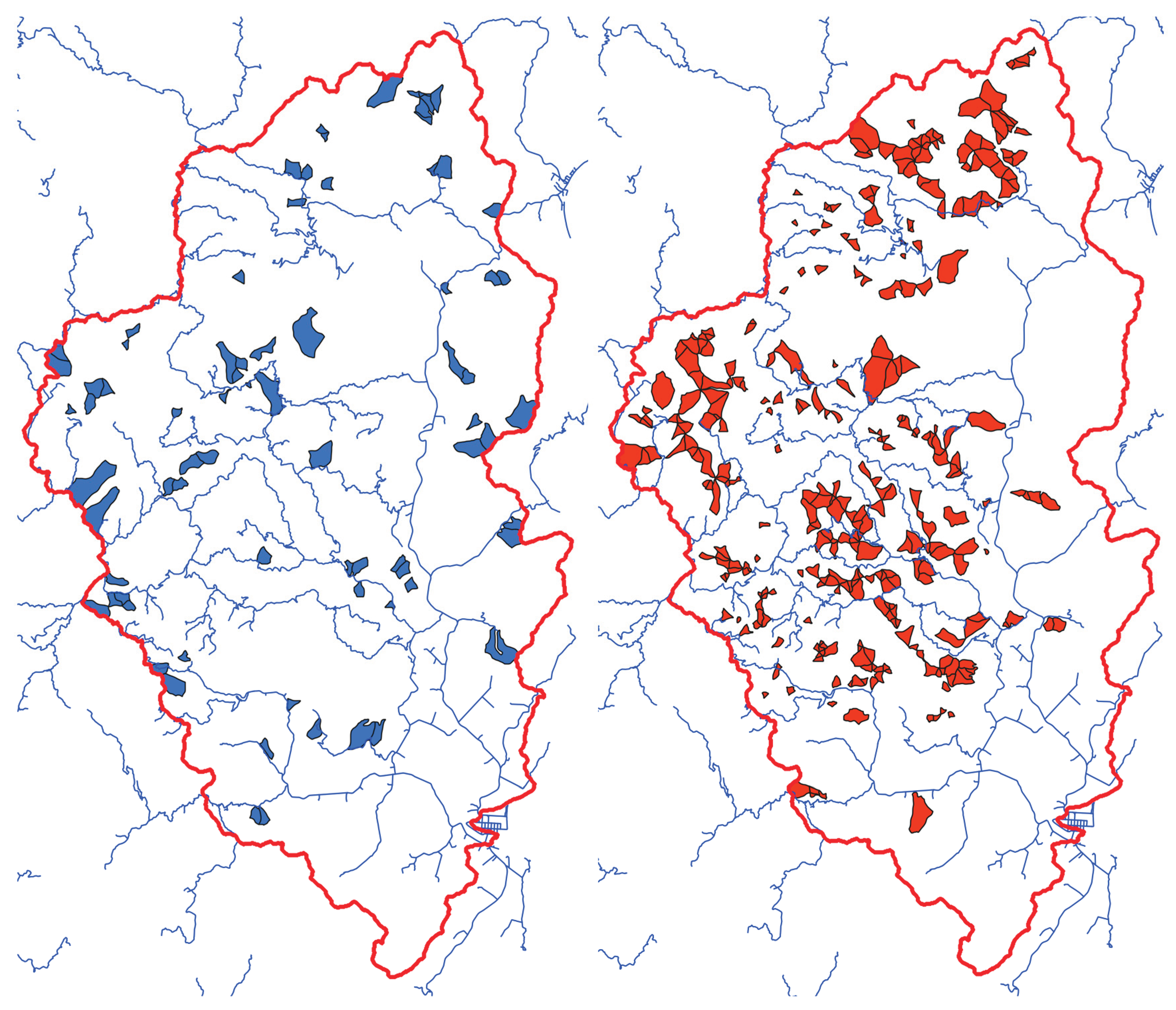
Increases in profitability as MHL increased can be explained by increases in the allowable cut. Figure 6c shows that the allowable cut along the planning horizon is the highest in the base unconstrained scenario compared with the MHL 10-50% scenarios, with a clear increase in allowable cut as the MHL increased. Similar to profitability, changes in the allowable cut for MHLs over 25% are relatively small. The relaxed solutions exhibited an overall similar pattern in the allowable cut (Figure 6d), although with some differences; notably, a higher allowable cut for the base scenario during the first two periods, declining below the MHL 20-50% scenarios in later periods.
Now that we know that profitability drops with lower values of MHL, driven by lower values of the allowable cut, we may delve into the reasons why this occurs. The first obvious reason is that imposing a maximum threshold area that could be harvested in a CMU at any single period will evidently impose restrictions that translate into reductions in profitability, e.g. imposing a 25% MHL on a CMU with mostly mature forests obliges postponing most of the harvest for subsequent periods, reducing overall profitability. The second reason is less evident, although probably more important than the first reason, which is related to the stands that are not harvested along the planning horizon. Figure 7 compares the stands unharvested under scenarios MHL 10-50% with 5% steps. Only a marginal area was left unharvested in the base scenario (100 ha, 0.31% of the total area), being very small units with high harvesting and roading costs, rendering harvesting unprofitable (Figure 7). Almost the same occurs with the relaxed MILP solution, where only 103 ha were left unharvested.
The areas left unharvested at the end of the planning horizon increase as the MHL becomes more restrictive (e.g. MHL 10% is more restrictive than MHL 25%) (Figure 7). The uncut areas decrease as the MHL increases: 16,324 ha (51% of the total forest estate) for MHL 10%, 9526 ha (30%) for MHL 15%, 3955 ha (12%) for MHL 20%, 2273 ha (7%) for MHL 25%, 1764 ha (6%) for MHL 30%, 1575 ha (5%) for MHL 35%, 1246 ha (4%) for MHL 40%, 886 ha (3%) for MHL 45%, 797 ha (2%) for MHL 50%. The area left unharvested in the MILP relaxed solution was lower than for the MILP solution but far from zero i.e. 10,522 ha (33%) for MHL 10%, 4675 ha (15%) for MHL 15%, 827 ha (3%) for MHL 20%, 120 ha (0.38%) for MHL 25%, 106 ha (0.33%) for MHL 30%, 106 ha (0.33%) for MHL 35%, 103 ha (0.32%) for MHL 40%, 103 ha (0.32%) for MHL 45% and 103 ha (0.32%) for MHL 50%.
The MILP and the MILP relaxed solutions provide us with an upper and lower bound of the unharvested area. At this time, we consider that an MHL of 25% seems reasonable in terms of profitability and allowable cut, particularly if the unharvested areas of the MILP could be harvested according to the MILP relaxed solution. An MHL of 25% seems reasonable compared with the other MHL scenarios because of its profitability and also because the unharvested area could be moved from a maximum of 2273 ha (7%) for the MILP solution to somewhere down to 120 ha (0.38% of the area of the forest estate) for the relaxed MILP solution. The IRR for an MHL of 25% would be 7.99% for the MILP and 8.60% for the relaxed MILP compared with 8.92% for the base scenario. It follows that for a catchment-oriented forest schedule such as the one proposed for the MHL 25%, the IRR would have to be sacrificed by 0.32-0.93% per annum.
The rationale for the uncut areas is that if harvested, the MILP problem will become unfeasible, mainly because some HSUs represent more than 25% of relatively small CMUs, so that harvesting one will surpass the MHL permitted. A visual depiction of the base scenario compared with the MHL 25% (both using the MILP solution) is shown in Figure 9. The base scenario shows that a high proportion of some CMUs are harvested in some periods, while only marginally harvested or not harvested in others. The MHL 25% scenario shows a more spatially balanced harvest schedule across CMUs.
In order to minimise the gap in profitability between the base and the 25% MHL scenarios, one alternative would be to use both the MILP and the relaxed MILP solutions for the 25% MHL, the second for those areas left unharvested in the first (Figure 7, bottom left). A more elegant approach, as presented in the next section, would be to relax the solution but only for those units unharvested in the MILP solution.
3.3. A semi-Relaxed MILP Solution
Based on the above, we constructed a new scenario considering our previous findings. This new scenario comprises catchment-oriented forest planning with no more than 25% of any Catchment Management Unit (CMU) to be harvested at any single period. The CMU is composed of hillslope units (HSU), which will be either harvested in a single period along the planning horizon or left unharvested. However, there is an exception. Some HSUs represent more than 25% of the area of the CMU, and therefore, under such a strict constraint, the HSUs are left unharvested, which becomes unrealistic. There are 47 out of 1123 HSUs (4.2%) under this condition, and the model relaxation allowed these particular HSUs to be partially harvested during the planning horizon, while all remaining HSUs were treated with binary variables.
The new semi-relaxed MILP scenario (NPV 5256 NZD/ha, IRR 8.55%) compares well with the base scenario (5727 NZD/ha, IRR 8.92%). Although there is a reduction in profitability (by 471 NZD/ha in NPV, and by 0.37% in IRR), the catchment-oriented harvest schedule seems to be marginally less profitable than the base scenario.
3.4. Incorporating Rainfall-Induced Landslides into Decision Making
Figure 4 (right) shows the RIL susceptibility across the study area, highlighting significant differences among HSUs (stands) and CMUs. Greatest RIL susceptibility is found within a strip running north to south along the slopes contributing to the main Uawa valley. Such high RIL susceptibilities should be considered in harvest scheduling. For instance, from the base scenario (Figure 8), it can be seen that a large proportion of some CMUs are harvested on a massive scale within a single period, even though their RIL susceptibilities are high. This is what has happened in the recent past, probably associated with older stands located in highly RIL-susceptible areas. Within the MHL 25% scenario, there must be a way to incorporate the RIL susceptibility into decision-making. A feasible alternative would be to spread the area in the WoV with high RIL susceptibility evenly throughout the planning horizon.
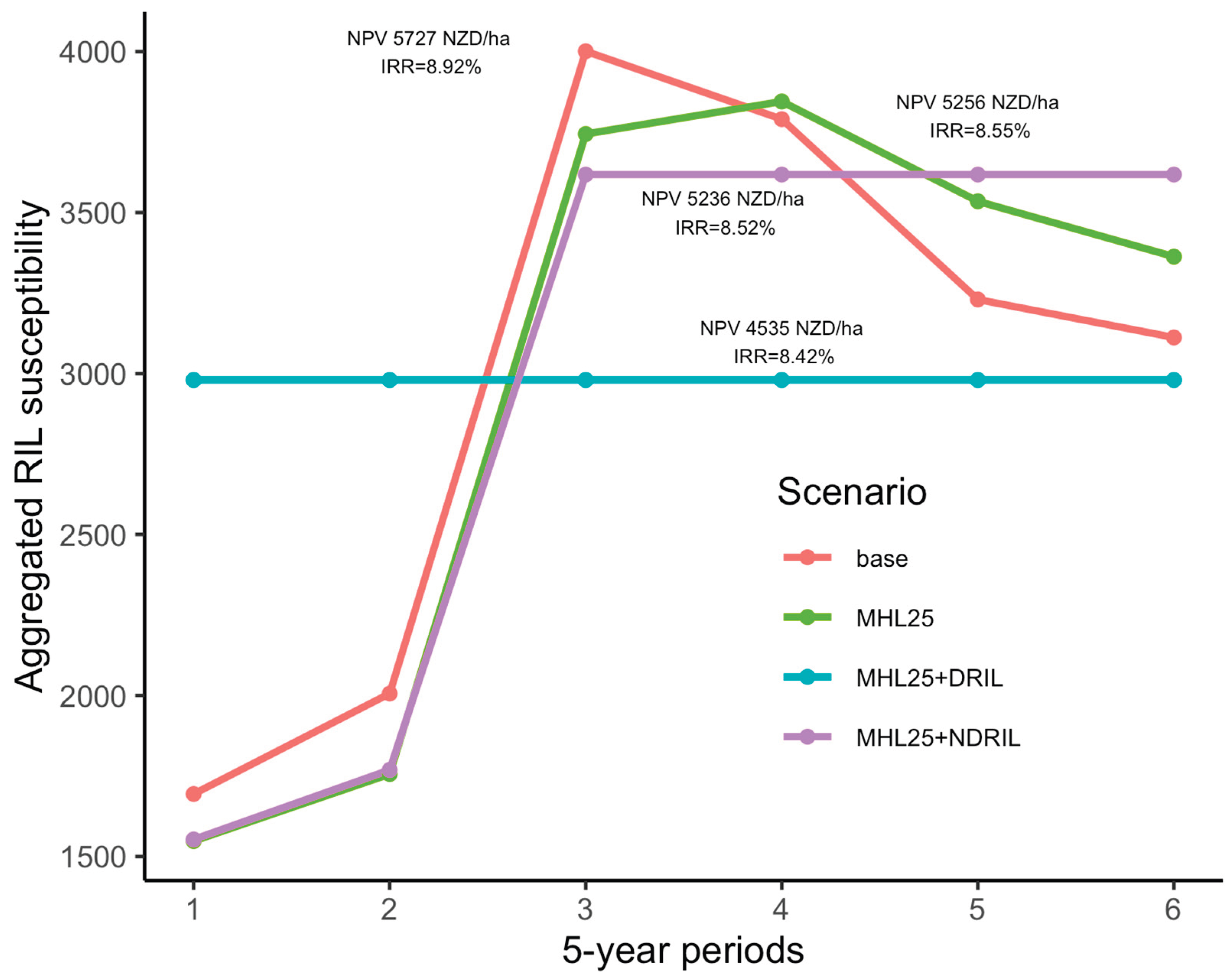
To model this, we ran a new scenario based on the MHL 25% by adding a proxy of RIL susceptibility as the weighted sum of area harvested times the HSU’s RIL susceptibility in a given period (see equation 6 above). Figure 9 compares the RIL susceptibility for the base scenario against the MHL 25% with non-declining (Equation 7) and declining (Equation 8) RIL susceptibility.
The base scenario with the highest profitability (NPV 5727 NZD/ha, IRR 8.92%) among all scenarios analysed showed the most variable aggregated RIL susceptibility along the planning horizon (Figure 9). The base scenario also showed the highest peak in aggregated RIL susceptibility in period 3. The MHL25% scenario (NPV 5256 NZD/ha, IRR 8.55%) was similar in aggregated RIL susceptibility to the base scenario, although with a slightly lower peak. When adding non-declining RIL susceptibility constraints to the MHL 25% scenario (NPV 5236 NZD/ha, IRR 8.52%), profitability reduced marginally compared with the MHL25% scenario, but RIL susceptibility stayed constant after period 3 with lower peaks compared to the base and MHL 25% scenarios (Figure 9). When adding declining RIL susceptibility constraints to the MHL 25% scenario, profitability was reduced the most compared to other scenarios (NPV 4535 NZD/ha, IRR 8.42%), although RIL susceptibility was kept constant over all six periods and lower compared to the peaks of all other scenarios. We found the base scenario to be the worst solution because of the high fluctuations from period to period in RIL susceptibility. The most conservative solution will be MHL 25% with declining RIL susceptibility constraints (MHL25+DRIL scenario), although with a relatively strong penalty on profitability. However, achieving constant RIL susceptibility demands harvesting below age 20 at the start of the planning horizon to make the solution feasible, rendering this option impractical. Therefore, we chose the MHL 25% with non-declining RIL susceptibility (MHL25 + NDRIL) as the best option because it improves on the MHL 25% at a marginal cost in profitability. The MHL25 + NDRIL scenario couples a sustainable allowable cut with constant aggregated RIL susceptibility achieved from period 3 onwards (Figure 9).
Figure 8.
Comparison of the harvested areas in the MILP solution for the MHL 25% (above) and the base (below) scenarios for each of the six 5-year periods that comprise the planning horizon. The MHL 25% scenario means that at most 25% of a Catchment Management Unit (CMU) could be harvested in any one 5-year period.
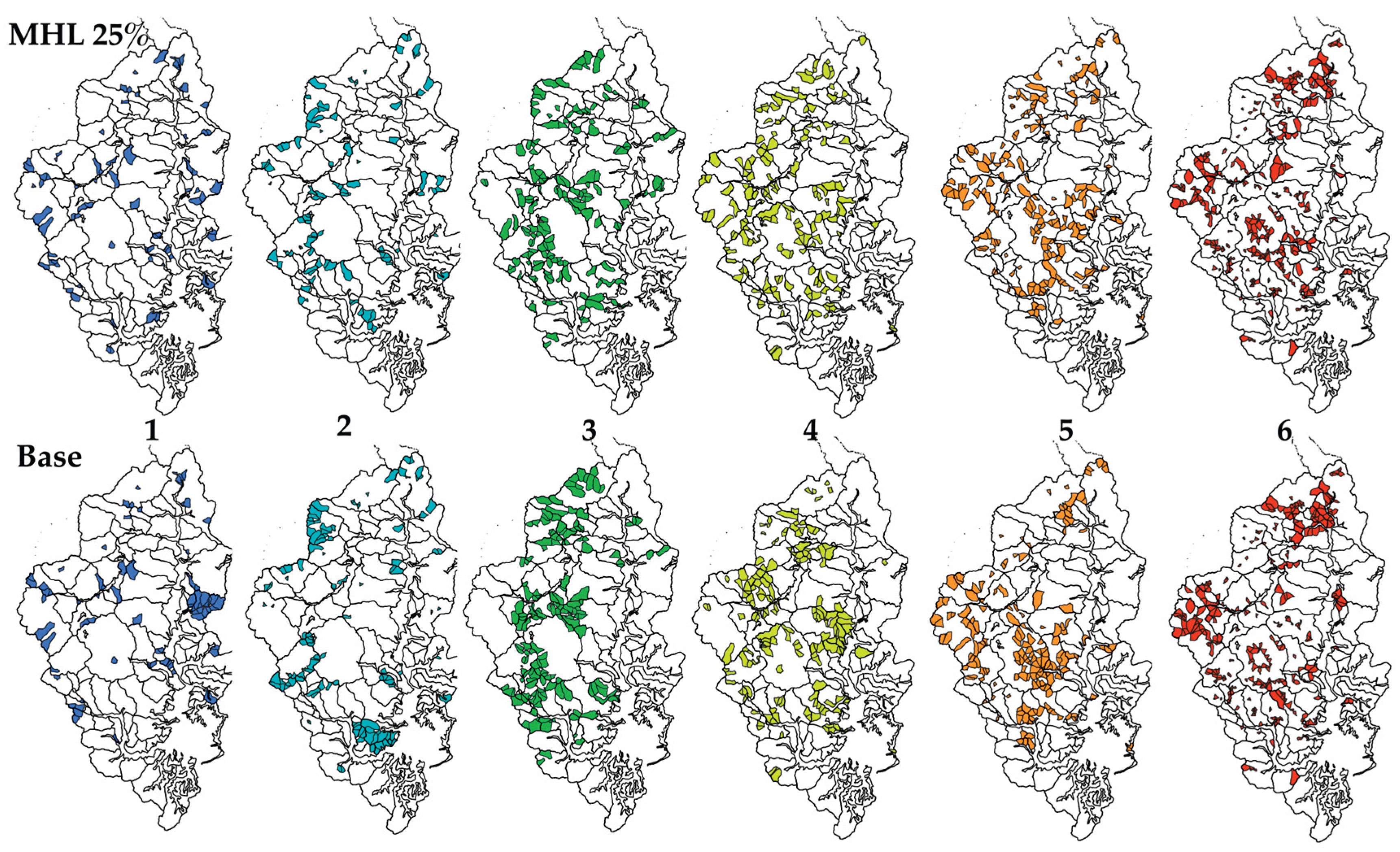
Figure 9.
A proxy of RIL susceptibility is calculated as the aggregated sum of harvested areas times each HSU’s RIL susceptibility. The plot compares the base scenario (red line) against the MHL 25% scenario (green line), the MHL 25% plus non-declining (MHL25+NDRIL, magenta line) and declining (MHL25+DRIL, light-blue line) aggregated RIL susceptibility. The MHL 25% scenario means that at most 25% of each Catchment Management Unit (CMU) could be harvested in any one 5-year period. Profitability metrics are also included: NPV (net present value), IRR (internal rate of return).
3.5. Our Best Solution for the Catchment-Oriented Harvest Schedule
The best catchment-oriented harvest schedule in our view is the one in which no more than 25% of each CMU is harvested in any single 5-year period (i.e. no more than 5% of each CMU in a year), applying a semi-relaxed MILP approach (i.e. most stands are either harvested or not in any single period, while a minority of stands are partially harvested over several periods), and with an aggregated RIL susceptibility that reaches a maximum which is kept constant in perpetuity. A constant RIL susceptibility would allow forest owners to spread landslide risk equally over time. Profitability is reduced from a maximum IRR of 8.92% for the base scenario to 8.52% for this “best” scenario. Figure 10 (a) shows the HSUs which will be harvested over several periods (yellow), compared with the HSUs entirely harvested in period 1 (blue). Successive letters (b) to (f) in Figure 10 show areas harvested in periods 2, 3, 4, 5, and 6.
The forest estate comprised 1123 HSUs within 89 CMUs, covering an area of 31,899 ha, 59% of the total area of the Uawa catchment. Twenty-five per cent of the HSUs were below 7.8 ha, 50% below 20.8 ha, and 75% below 39.0 ha. The maximum HSU size was 182 ha. The 89 CMUs range in size from 36 to 2971 ha with a mean of 697 ha. Not all CMUs were completely covered with plantations. Thirty-seven per cent of all CMUs had complete forest cover, while 25% had less than 13% forest cover. On average, CMUs had a 63% forest cover. The fact that 63% of all CMUs had partial forest cover meant that the constraint that no more than 25% of the CMU could be harvested at any single period was not as harsh as previously thought. In fact, although the maximum area harvested in each CMU in any single period is 25%, the minimum is 0 and the mean moves from 9-19% (Table 3).
The area harvested per period was lower during the first two periods compared with later periods, probably associated with an initial age distribution where young ages were dominant (Table 3). Timber flow, income and aggregated RIL susceptibility progressively increased along the planning horizon to peak and even out from period 3 onwards, moving towards a more balanced age distribution by the end of the planning horizon (Table 4, cells in light green). The last row of the stock table (Table 4) shows some cells in grey. These correspond to the 155 ha (81 stands, 0.48% of the total forest estate) that were left unharvested because these units were relatively small (range 0.04-17.76 ha, mean of 2.57 ha) with high harvesting and roading costs, rendering their harvest unprofitable.
4. Discussion
The management of radiata pine plantations has been shown to be highly profitable, particularly in the North Island of New Zealand. Our research hypothesis that the profitability of catchment-oriented harvest planning (IRR 8.52%) would not be drastically different from the business-as-usual policy (IRR 8.92%) was confirmed. These IRRs observed are considered to be robust for radiata pine and other forest species (Douglas-fir, eucalypts and blackwood) in New Zealand (Manley, 2018).
In our catchment-oriented harvest scheduling approach, land is divided not according to the limits of stands historically planted but according to hillslopes (HSUs), which behave hydrologically as a unit. These hillslope units typically represent Order 1 or 2 catchments (“headwater streams”), dominated by steep slopes and high stream gradients, where erosion is the dominant landscape process. These HSUs are fully contained within catchment management units (CMUs), which discharge through a “pour point” onto built and natural environments in the downstream transfer and depositional zones.
Once HSUs and CMUs are defined, a limit can be placed on the maximum area that can be clearfell harvested in any single period along the planning horizon within each CMU. We have called this threshold the Maximum Harvest Level (MHL), expressed as a fraction of any CMU, e.g. MHL 15% means that not more than 15% of any CMU could be harvested at any single 5-year period. For the base scenario, we ran a tactically explicit harvest scheduling model maximising the NPV subject to non-declining yield constraints. We then ran further scenarios in which MHL constraints were added to the base simulation, testing MHLs in a series from 10% to 50% with 5% steps. Thus, for these new scenarios, we maximised the NPV subject to non-declining yield and MHL constraints. Imposing the MHL constraints in the range 10-20% drastically reduced profitability. In comparison, for MHLs 25% and larger, differences in profitability with the base scenario were relatively small. Based on the results of our study, we consider that an MHL of 25% struck a good balance between profitability and limiting the maximum area that could be harvested in any CMU in any single period.
When running the tactical harvest scheduling model under the MHL 25% constraint, we found that 47 out of 1123 HSUs were left unharvested at the end of the planning horizon because they represented more than 25% of the CMU. This is something likely to happen in reality, where CMUs are relatively small in area and composed of a small number of HSUs, or when HSUs are large compared with the CMU size. As these HSUs are only a small proportion of the total number of HSUs (4.2%), we relaxed the solution for those particular cases, i.e. instead of using binary 0-1 variables, we used continuous variables in the 0-1 range. As an example, an HSU unit left unharvested (binary variable equal to zero) could be relaxed, allowing the decision variable to take fractional values, meaning that the stand could be harvested over several periods in partialities. For example, 0.3 means that 30% of that HSU would be harvested in that period. Such a strategy of using binary variables for most of the forest estate and continuous fractional variables for the units that exceeded 25% of the CMU proved to be technically and financially feasible. This condition of small CMUs or CMUs with only a few large HSUs is likely to occur in other forest estates, suggesting that relaxing the solution is a useful option.
A proxy of rainfall-induced landslide susceptibility was constructed as the product of the area harvested times RIL susceptibility calculated for each period. This proxy was then forced to be as constant as possible. This strategy would allow the spreading of risk from rainfall-induced landslides along the planning horizon, avoiding years where stands in the WoV had high RIL susceptibility, followed by years where stands in the WoV had low RIL susceptibility. We achieved such a condition by applying declining RIL susceptibility constraints, i.e. ensuring that the aggregated value of area harvested times RIL probabilities declined or stayed the same from one period to the next. However, this strategy proved to be impractical, demanding harvesting stands below 20 years of age during the first 5-year period in order to render the problem feasible. Our second option was applying non-declining aggregated RIL susceptibility from one period to the next. We found this strategy to be more grounded in reality, since aggregated RIL susceptibility was constant from period 3 onwards and overall lower and less fluctuating than for the base and MHL 25% scenario (Figure 9). Given that the information about RIL susceptibility is widely available at the HSU level, it follows that it could be routinely included in tactical harvest scheduling planning in the Gisborne Region.
The “Ministerial Inquiry into Land Use causing woody debris and sediment-related damage in Tairāwhiti and Wairoa” (MILU) recommended imposing limits on the maximum clear-cut size (40 ha) and also that no more than 5% of a catchment is harvested each year (Ministry for the Environment (MfE), 2023). Our model aligns well with this statement. The median of our 1123 HSUs is 20 ha, while 75% are below 39 ha, and for those units exceeding 40 ha, we can enforce not harvesting more than that amount every year with continuous fraction variables in the range 0-1. In relation to the second part of the statement, i.e. no more than 5% of each CMU is harvested each year, our results also align well because an MHL of 25% means that over the 5-year planning period, the clearfell harvest is limited to 25%, or 5% per year.
Adjacency constraints are a common practice in forest management in other areas around the world, which prevent contiguous units from being harvested at the same time so that the maximum size of clearcuts does not exceed statutory or policy limits (O’Hara et al., 1989). These constraints are now being routinely used in harvest scheduling planning for erosion control, biodiversity conservation and reducing the negative impacts of storms on forests, among others (Boston & Bettinger, 2002; Boston & Sessions, 2006; Loehle, 2000; O’Hara et al., 1989). In our catchment-oriented harvest scheduling plan, we have not considered adjacency constraints because the HSUs represent sub-catchments which are hydrologically independent of other HSUs. It is worth asking whether an adjacency constraint will have any effect on rainfall-induced landslide risk when using the FCP methodology.
Where neighbouring HSUs drain to different streams, it would make no sense to impose adjacency constraints to reduce RIL susceptibility. However, there might be some space here to consider the case of HSUs that contribute to the same water and woody debris flow pathway—for example, those on opposite slopes of the same subcatchment; in that case, adjacency may play a role. We suggest here that adjacency constraints might be necessary for a reduced subset of HSUs in order to harvest these units in different periods.
Implicitly, the MHL 25% scenario implies a greenup period of 5 years. Consider that during the first 5-year period, no more than 25% of the CMU will be harvested. During the second period, this condition will be repeated. Then, at least some units harvested during the first and second period will be neighbours, where the ones harvested during the first period will have a 5-year-old plantation. Phillips et al. (2024) define the concept of “Window of vulnerability” as the time lapse following forest removal when steep land is vulnerable to rainfall-induced landslides. This window of vulnerability may vary between 1-8 years after clearfelling, although years 2-4 seem to be the most critical. In our case, we consider that five years would allow radiata pine plantations to reach 6-8 m in height and achieve complete canopy cover after planting in the Tairāwhiti|Gisborne region, which is a condition for landslide density to drastically drop (Phillips et al., 2024).
Several potential limitations of this study warrant further investigation. First of all, reshaping current forest stands to HSUs may take a few years and some planning for harvesting and the plantation establishment. Therefore, taking the decision today to start a catchment-oriented harvest scheduling will not give immediate results and will need a transition period. Second, two or more forest owners may be present in a given CMU, and therefore, harvest scheduling would need coordination between them. We may find that some CMUs are only controlled by one forest owner, and that some CMUs may have the same common owners, where trade-offs might be possible.
Another counterargument that could arise is that harvesting HSUs spread over the landscape might impose higher operational costs. Our take on this is that the HSUs are big enough so that operational costs will not increase. In fact, the VCM cost model (Manley et al., 2015; Park et al., 2012) shows that for areas greater than 20 ha, harvesting and roading costs only marginally increase per m3. In our particular case, 25% of the HSUs were below 7.8 ha, 50% below 20.8 ha, 75% below 39.0 ha, and the maximum HSU size was 182 ha.
A further counterargument against a catchment-oriented harvest schedule is that harvesting systems may not be well-suited to HSU-based harvesting units. We argue that, on the contrary, a catchment-oriented harvest schedule is well-suited to conventional steepland harvesting systems. Skylines set at ridges are routinely used to harvest steepland forests in New Zealand (Amishev et al., 2014). However, this method is generally limited to haul distances of 300–500 m (Spinelli et al., 2021). These ridge-to-ridge distances are well within values for many of the HSUs in the Uawa catchment. For large HSUs, those distances could be achieved by subdividing the HSUs. Detailed operational planning is needed to implement catchment-oriented harvesting, particularly in broken terrain, but difficulties are likely surmountable in most cases.
In tactical planning, prioritising harvesting areas near existing roads is a common strategy to minimise road construction, transportation, and streamline harvest operations (Wells, 2002). In our study, we implemented a “roads-first-policy” by assuming that any HSU whose centroid was within a 200 m buffer of primary roads would be excluded from new road construction. As a result, most units harvested during the initial periods were clustered near existing roads, while those scheduled for later harvest were generally located farther away (Figure A.1).
The range of piece sizes resulting from the extended harvesting age may pose operational challenges. The tactical planning shows that some harvesting along the planning horizon will involve trees 45+ years reaching up to 80 cm in dbh. Difficulties can arise specifically in the mechanised felling of trees. Fully mechanised tree harvesting is generally limited to trees with a dbh of 60–80 cm, depending on the machine type. Feller bunchers typically handle trees up to 60–65 cm dbh, with productivity and safety declining near the upper limit. Cut-to-length harvesters, particularly larger models used for final felling of conifers, can process trees up to 75–80 cm dbh, although performance and efficiency decrease at these extremes. Based on the above, some operational difficulties and increases in harvesting costs are expected to arise as a result of piece size, particularly on HSUs where the rainfall-induced landslide probability is high.
Our model, while currently theoretical and not yet field-tested, suggests that catchment-oriented harvest scheduling is technically and financially feasible. We predict that reshaping stands to conform to hillslope units and harvesting no more than 25% of each CMU over 5 years (5% per year) may increase landscape resilience and reduce rainfall-induced landslide susceptibility. This catchment-oriented approach would likely be more ecologically and socially acceptable than traditional unconstrained clearcuts with only marginal reductions in profitability.
5. Conclusions
Catchment-oriented harvest scheduling compares well with traditional systems oriented to large clearcuts, but with clear advantages in reducing rainfall-induced landslides susceptibility. Catchment-oriented harvest scheduling would imply reshaping current stands to conform to hillslope units (HSUs) within Catchment Management Units (CMUs). These HSUs correspond to small Order 1 or 2 catchments within CMUs. In our case study, 75% of the HSUs were below 39.0 ha, with a maximum HSU size of 182 ha. However, the upper quartile over 39 ha could be subdivided to be harvested over several periods. We found that restricting harvest to no more than 25% of any CMU at any single 5-year period would strike a balanced trade-off between profitability and landscape susceptibility. Forcing the RIL proxy (area harvested times RIL susceptibility) to stay constant once the forest is regulated would allow the spreading of landslide risk evenly across the planning horizon. Forest owners’ concerns that catchment-oriented harvest scheduling would need coordination across ownerships, that reshaping stands would take time, effort and money, and that operational costs would increase as a result of spreading the harvesting units over the landscape, do not seem to be insurmountable.
Author Contributions
Conceptualisation, H.E.B., M.B., M.D.; Databases, M.B., R.B. and B.R., methodology, H.E.B., M.B., M.D.; software, H.E.B. and R.B.; validation, H.E.B., M.B., M.D.; formal analysis, H.E.B., M.B., M.D.; investigation, H.E.B., M.B., M.D.; data curation, M.B., R.B. and B.R.; writing—original draft preparation, H.E.B., M.B., M.D. and B.R.; writing—review and editing, H.E.B., M.B., M.D., R.B. and B.R. All authors have read and agreed to the published version of the manuscript.
Funding
This research was mainly supported by the University of Canterbury, the University of Chile, and the Forestry Catchment Planner project.
Data Availability Statement
The yield tables used to develop the model are proprietary data owned by the New Zealand Ministry of Primary Industries and are publicly available.
Acknowledgments
The authors gratefully acknowledge the expert advice of Rien Visser, Campbell Harvey and Karen Bayne, whose insights were invaluable in aligning the tactical planning for the Uawa catchment with practical, on-the-ground realities.
Conflicts of Interest
The authors declare no conflicts of interest.
Appendix A
Figure A1.
HSUs harvested during the first 5-year period (left panel) are mostly clustered around primary roads, while some HSUs harvested during the last 5-year period (right panel), particularly small ones, are located at a greater distance from roads.
Figure A1.
HSUs harvested during the first 5-year period (left panel) are mostly clustered around primary roads, while some HSUs harvested during the last 5-year period (right panel), particularly small ones, are located at a greater distance from roads.
References
- Amishev, D., Basher, L, Phillips, C., Hill, Spencer, Marden, M., Bloomberg, M, & Moore, J. (2013). New Forest Management Approaches to Steep Hills Prepared for the Ministry for Primary Industries. http://www.mpi.govt.nz/news-resources/publications.aspx.
- Bloomberg, M., Cairns, E., Du, D., Palmer, H., & Perry, C. (2019). Alternatives to clearfelling for harvesting of radiata pine plantations on erosion-susceptible land. NZ Journal of Forestry, 64(3), 33–39.
- Bloomberg, M., & Urlich, S. (2025). Lessons for steepland forestry harvesting in New Zealand from recent Resource Management Act prosecutions. NZ Journal of Forestry, 70(2), 3–9.
- Boston, K., & Bettinger, P. (2002). Combining Tabu Search and Genetic Algorithm Heuristic Techniques to Solve Spatial Harvest Scheduling Problems. Forest Science, 48, 35–46. [CrossRef]
- Boston, K., & Sessions, J. (2006). Development of a spatial harvest scheduling system to promote the conservation between indigenous and exotic forests. International Forestry Review, 8(3), 297–306. [CrossRef]
- Crozier, M. J. (2017). A proposed cell model for multiple-occurrence regional landslide events: Implications for landslide susceptibility mapping. Geomorphology, 295, 480–488. [CrossRef]
- Erber, G., Visser, R., Leitner, S., Harrill, H., Spinelli, R., Picchio, R., Varch, T., & Stampfer, K. (2025). Advances in Cable Yarding: a Review of Recent Developments in Carriers for Mobile Skyline Cable Yarding. Current Forestry Reports, 11(1), 14. [CrossRef]
- Gellis, A., Fitzpatrick, F., & Schubauer-Berigan, J. (2016). A Manual to Identify Sources of Fluvial Sediment. https://nepis.epa.gov/Exe/ZyPDF.cgi/P100QVM1.PDF?Dockey=P100QVM1.PDF.
- Gurobi Optimization, L. (2024). Gurobi Optimizer Reference Manual. https://www.gurobi.com.
- Leitner, S., Spinelli, R., Bont, L. G., Vidoni, R., Renzi, M., & Schweier, J. (2023). Technical, Safety and Environmental Challenges in the Electrification of Cable Yarding Equipment. Current Forestry Reports, 9(4), 263–275. [CrossRef]
- Loehle, C. (2000). Optimal control of spatially distributed process models. Ecological Modelling, 131(2–3), 79–95. [CrossRef]
- Manley, B. (2018). Discount rates used for forest valuation – results of 2017 survey. NZ Journal of Forestry, 63(2), 35–43.
- Manley, B. (2021). Afforestation Economic Modelling. Final Report Prepared for Ministry for Primary Industries. http://www.mpi.govt.nz/news-and-resources/publications/.
- Manley, B., Morgenroth, J., & Visser, R. (2015). What proportion of the small-scale owners’ estate in the North Island is likely to be harvested? New Zealand Journal of Forestry, 60(3), 26–34.
- MapHQ. (2024). Forestry Catchment Planner 1.0. https://www.forestrycatchmentplanner.nz/.
- Massey, C., Leith, K., Robinson, T.R., Lukovic, B., McColl, S., Carey-Smith, T., Rosser, B., Wotherspoon, L., Smith, H., Betts, H., Buxton, R., & Bidmead, J. (2025). What controlled the occurrence of more than 116,000 human-mapped landslides triggered by Cyclone Gabrielle, New Zealand? Landslides, 1-20. [CrossRef]
- Ministry for the Environment (MfE). (2023). Outrage to optimism : report of the Ministerial Inquiry into land uses associated with the mobilisation of woody debris (including forestry slash) and sediment in Tairāwhiti/Gisborne District and Wairoa District. Ministerial Inquiry into Land Uses in Tairāwhiti and Wairoa. https://environment.govt.nz/assets/Outrage-to-optimism-superseded.pdf.
- Mologni, O., Grigolato, S., & Cavalli, R. (2016). Harvesting systems for steep terrain in the Italian Alps: state of the art and future prospects. Contemporary Engineering Sciences, 9, 1229–1242. [CrossRef]
- MPI (2025). Erosion Susceptibility Classification by class & area of plantation forestry (excluding Department of Conservation Land). https://www.mpi.govt.nz/dmsdocument/29804-Erosion-Susceptibility-Classification-by-class-area-of-plantation-forestry-excluding-Department-of-Conservation-Land.
- MWLR. (2025). NZLRI Land Use Capability 2021. https://lris.scinfo.org.nz/layer/48076-nzlri-land-use-capability-2021/.
- NZFOA. (2024). Facts and Figures 2023-2024 : New Zealand Plantation Forest Industry (pp. 1–63). https://www.nzfoa.org.nz/images/FOA_Facts_and_Figures_2023-2024_-_Web_file.pdf.
- O’Hara, A., Faaland, B., & Bare, B. (1989). Spatially constrained timber harvest scheduling. Can. J. For. Res., 19, 715–724. [CrossRef]
- Park, D., Manley, B., Morgenroth, J., & Visser, R. (2012). What proportion of the forest of small-scale owners is likely to be harvested-a Whanganui case study. In NZ Journal of Forestry (Vol. 57, Issue 3).
- Paul, T., & Wakelin, S. (2024). New Zealand’s planted forests–Carbon stocks and yield in fast growing exotic tree plantations of the Southern Hemisphere. Trees, Forests and People, 16. [CrossRef]
- Phillips, C., Betts, H., Smith, H. G., & Tsyplenkov, A. (2024). Exploring the post-harvest ‘window of vulnerability’ to landslides in New Zealand steepland plantation forests. Ecological Engineering, 206. [CrossRef]
- R Core Team. (2024). R: A Language and Environment for Statistical Computing (R Foundation for Statistical Computing, Ed.). R Foundation for Statistical Computing.
- Rosser, B., Massey, C., Lukovic, B., Dellow, S., & Hill, M. (2021). Development of a Rainfall-Induced Landslide Forecast Tool for New Zealand. In N. Casagli et al. (Ed.), Understanding and Reducing Landslide Disaster Risk. ICL Contribution to Landslide Disaster Risk Reduction. (pp. 273–277). Springer. [CrossRef]
- Snelder, T. H., & Biggs, B. J. F. (2002). Multiscale river environment classification for water resources management. Journal of the American Water Resources Association, 38(5), 1225–1239. [CrossRef]
- Spinelli, R., Magagnotti, N., Cosola, G., Grigolato, S., Marchi, L., Proto, A. R., Labelle, E. R., Visser, R., & Erber, G. (2021). Skyline tension and dynamic loading for cable yarding comparing conventional single-hitch versus horizontal double-hitch suspension carriages. International Journal of Forest Engineering, 32(S1), 31–41. [CrossRef]
- Taha, H. (2007). Operations Research: An Introduction (D. George, Ed.; Eighth Edition). Pearson Prentice Hall.
- Wells, C. (2002). Forest harvesting roads: meeting operational, social and environmental needs with efficiency and economy. In T. Enters, P. Durst, G. Applegate, P. Kho, & G. Man (Eds.), Applying reduced impact logging to advance sustainable forest management : International conference proceedings, 26 February to 1 March 2001, Kuching, Malaysia (p. 311). FAO. https://www.fao.org/4/ac805e/ac805e07.htm#bm07.
Figure 1.
Waihapua Forest, Northern Hawkes Bay, after Cyclone Bola in 1988 (above) and 2025 (below). Source: Garth Eyles & James Powrie.
Figure 1.
Waihapua Forest, Northern Hawkes Bay, after Cyclone Bola in 1988 (above) and 2025 (below). Source: Garth Eyles & James Powrie.
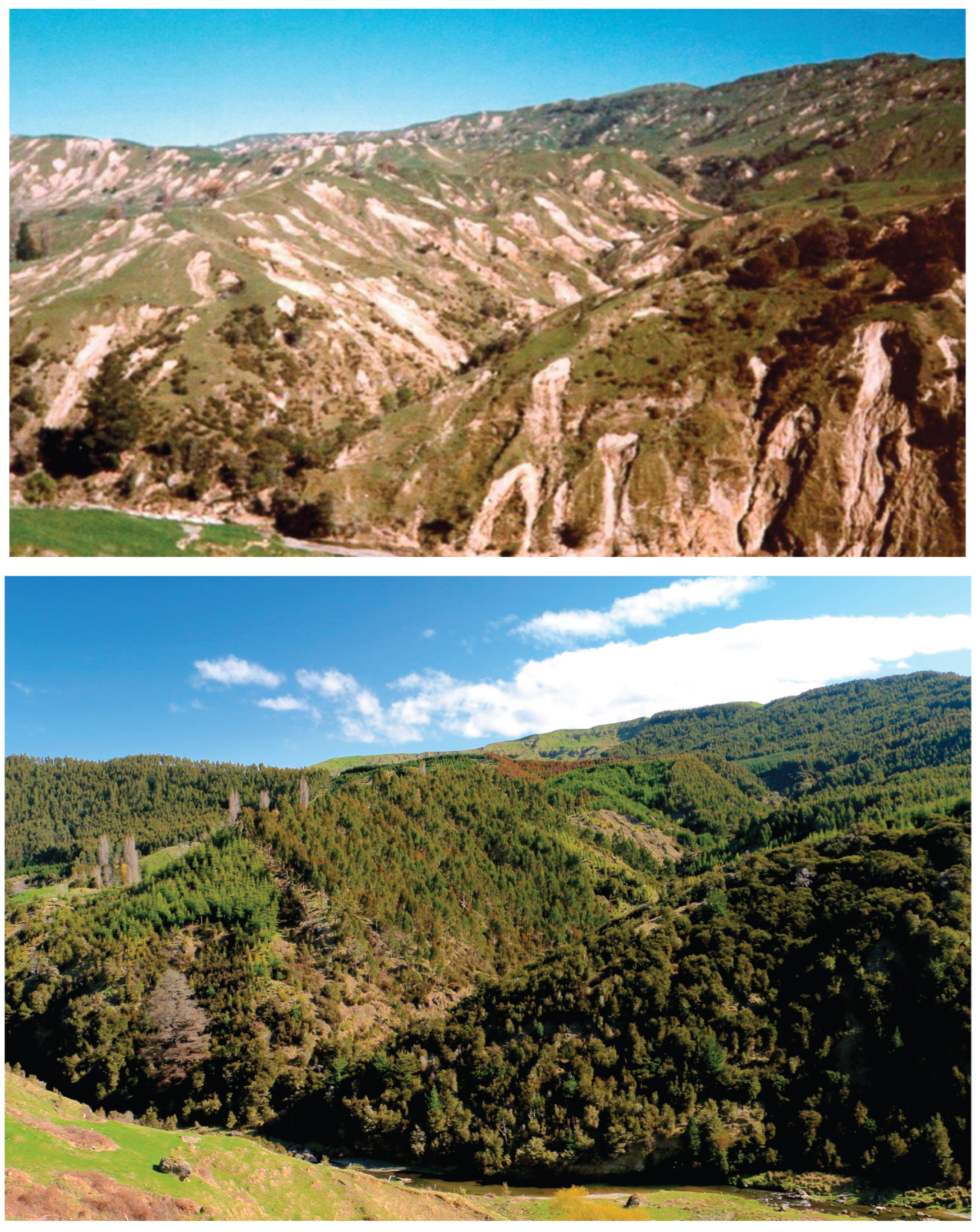
Figure 2.
A typical scale of clearfelling areas on highly erosion-susceptible land in Tairāwhiti|Gisborne, 2018. Source: D. Townsend, GNS Science; 11 July 2018.
Figure 2.
A typical scale of clearfelling areas on highly erosion-susceptible land in Tairāwhiti|Gisborne, 2018. Source: D. Townsend, GNS Science; 11 July 2018.
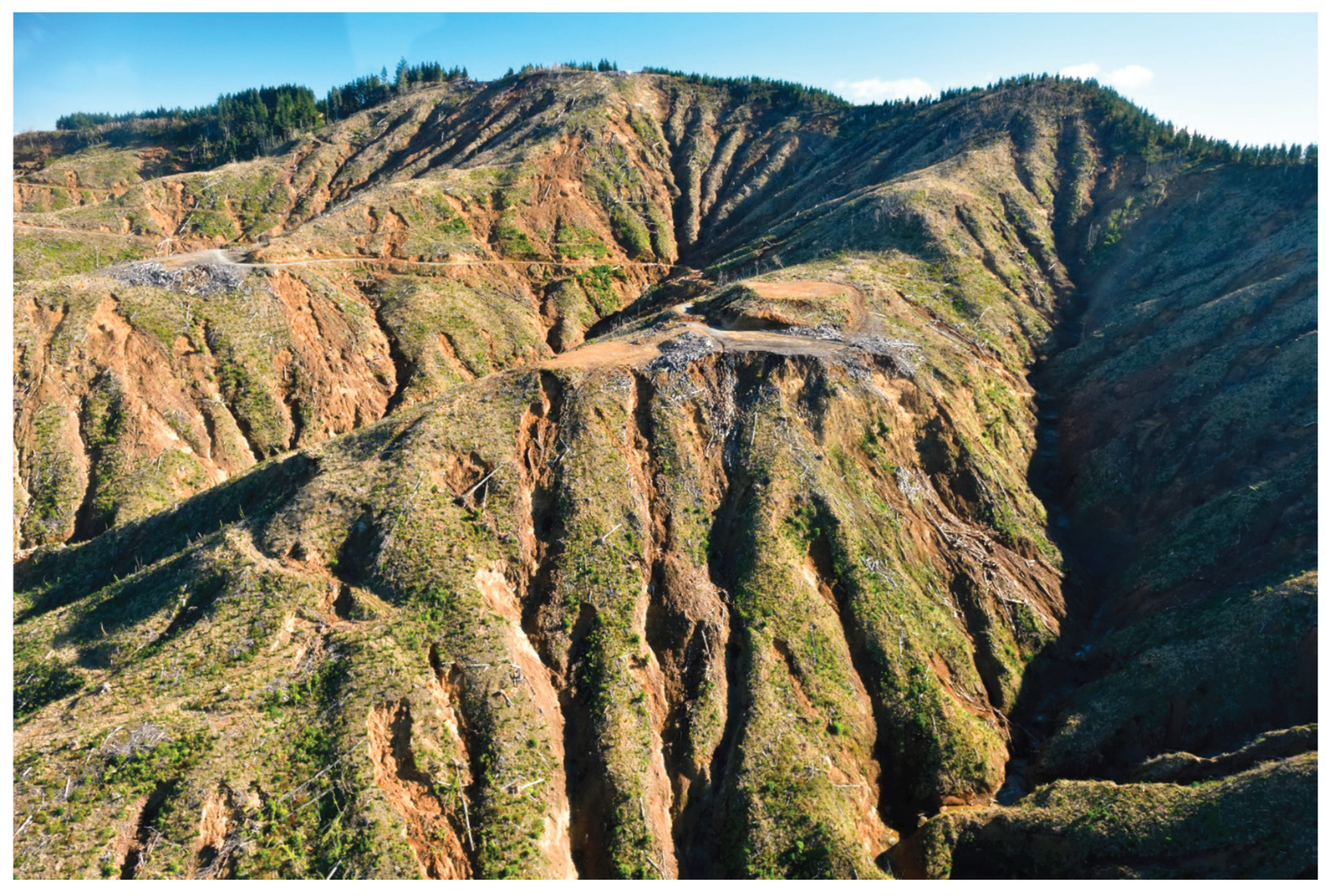
Figure 3.
Location and overall view of the Uawa catchment. The red dot in (a) represents the location of the Uawa catchment within the Gisborne Region of New Zealand. Colours in (a) represent the Gisborne (green), Hawkes Bay (blue), Nelson (magenta), Tasman (pink) and Marlborough (grey) regions. The Uawa catchment is represented in (b) and (c) by a red outline polygon and the coast by a grey line. In (b), forest plantations are represented by light green and highways by a blue line, while primary roads are represented by a black line. In (c), the hillshade model illustrates the broken terrain of the Uawa catchment. CRS: NZGD2000/New Zealand Transverse Mercator 2000.
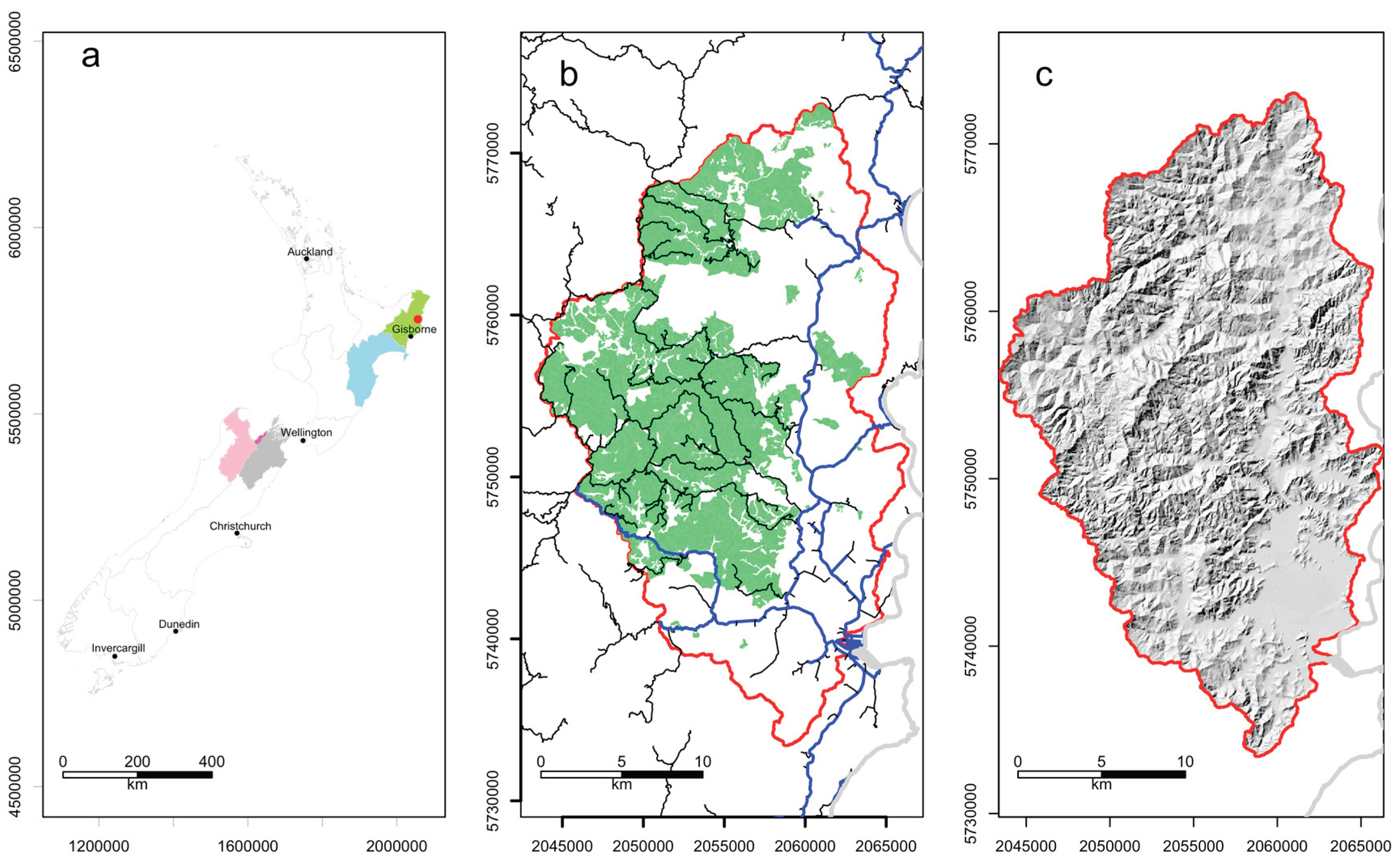
Figure 4.
CMUs, HSUs, slopes, forest ages and rainfall-induced landslide susceptibility. A red outline polygon represents the Uawa catchment, CMUs are defined by thick black lines, while HSUs are defined by thin black lines.
Figure 4.
CMUs, HSUs, slopes, forest ages and rainfall-induced landslide susceptibility. A red outline polygon represents the Uawa catchment, CMUs are defined by thick black lines, while HSUs are defined by thin black lines.
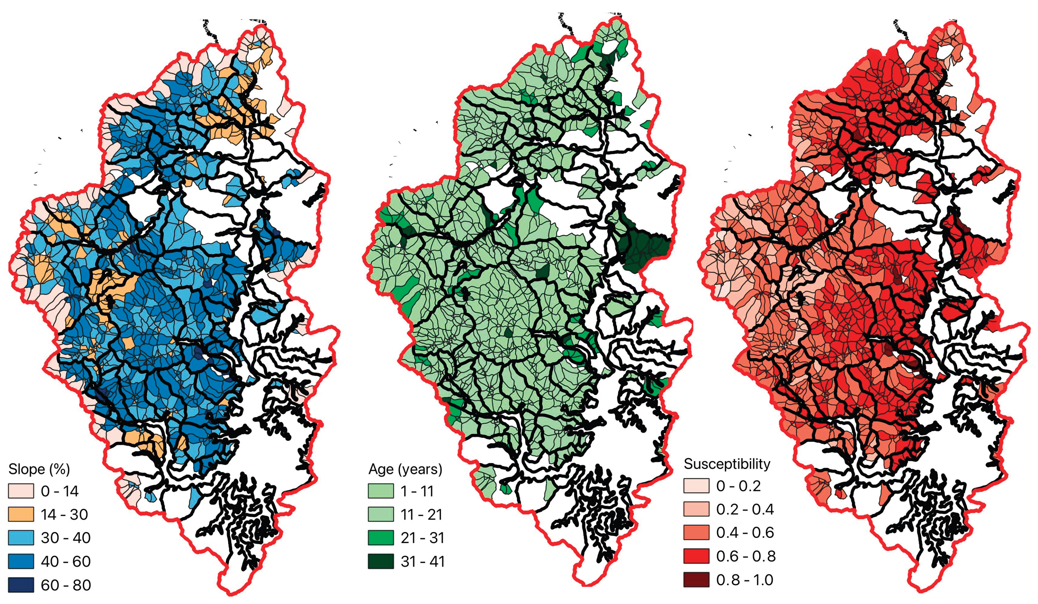
Figure 5.
Total recoverable volume and log outturn, versus harvesting age.
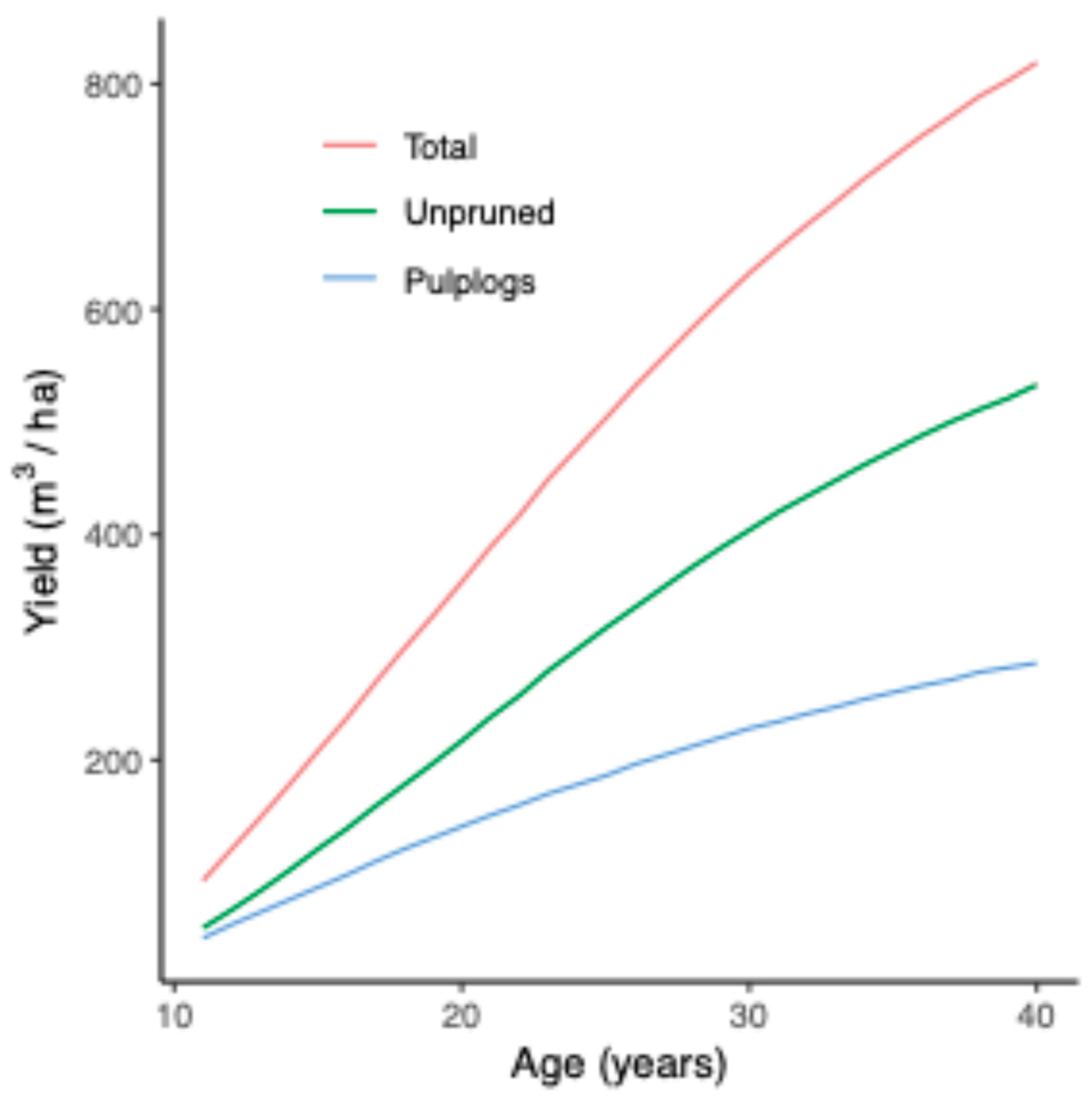
Figure 6.
Comparison of profitability and allowable cut for different harvest schedules considering Maximum Harvest Levels (MHL) within each Catchment Management Unit (CMU). The MHLs displayed are 10% to 50% (with 5% steps) of the area of each CMU that could be harvested at any one period. (a) and (c) show the MILP solutions, while (b) and (d) show the relaxed solutions.
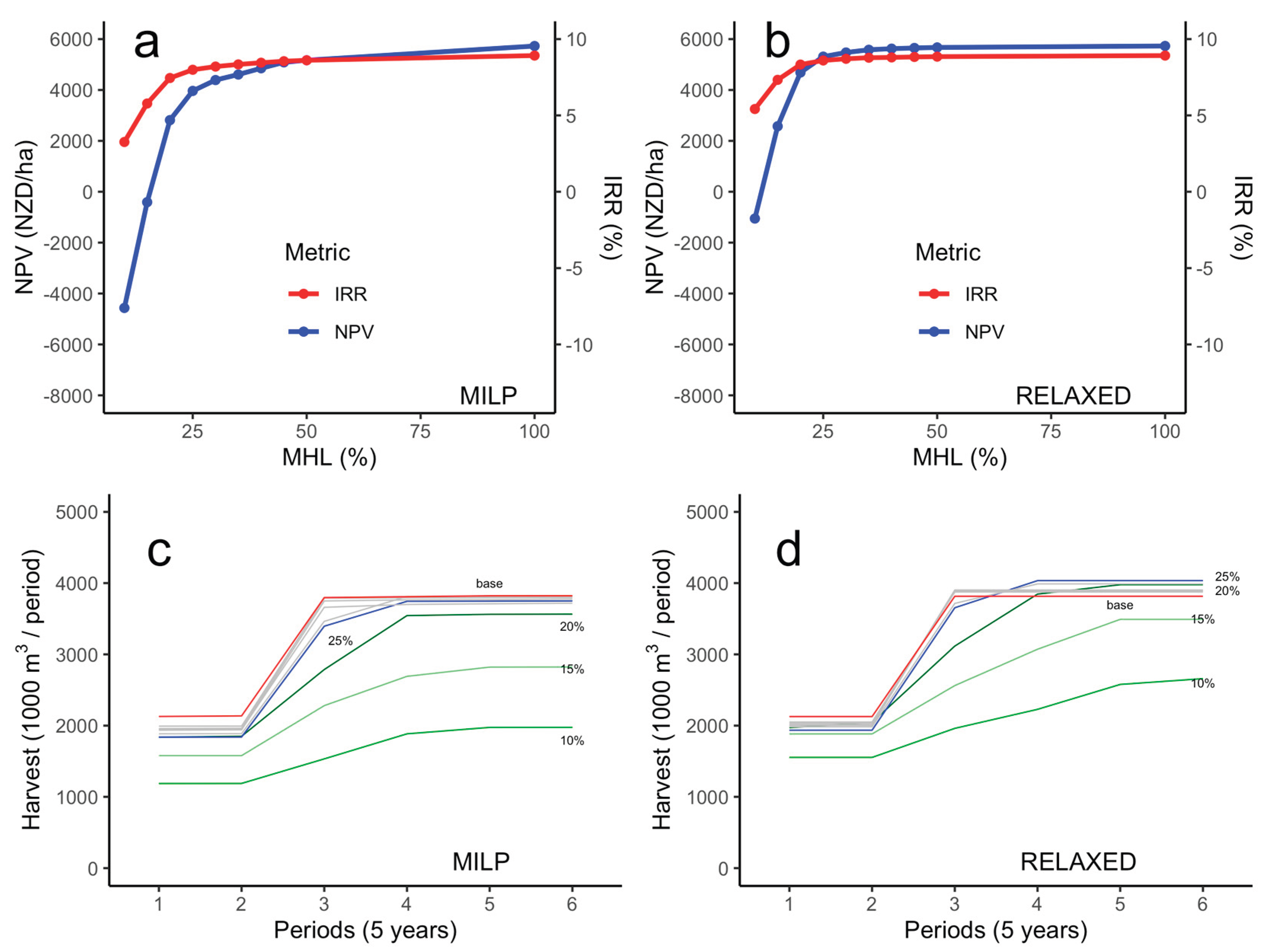
Figure 7.
Unharvested areas along the planning horizon for the base and the Maximum Harvest Level (MHL) scenarios. An MHL of 15% means that the maximum proportion of a catchment management unit (CMU) that could be harvested at any one 5-year period is 15%. The areas in red became unharvested because, if harvested, the MILP problem would become infeasible.
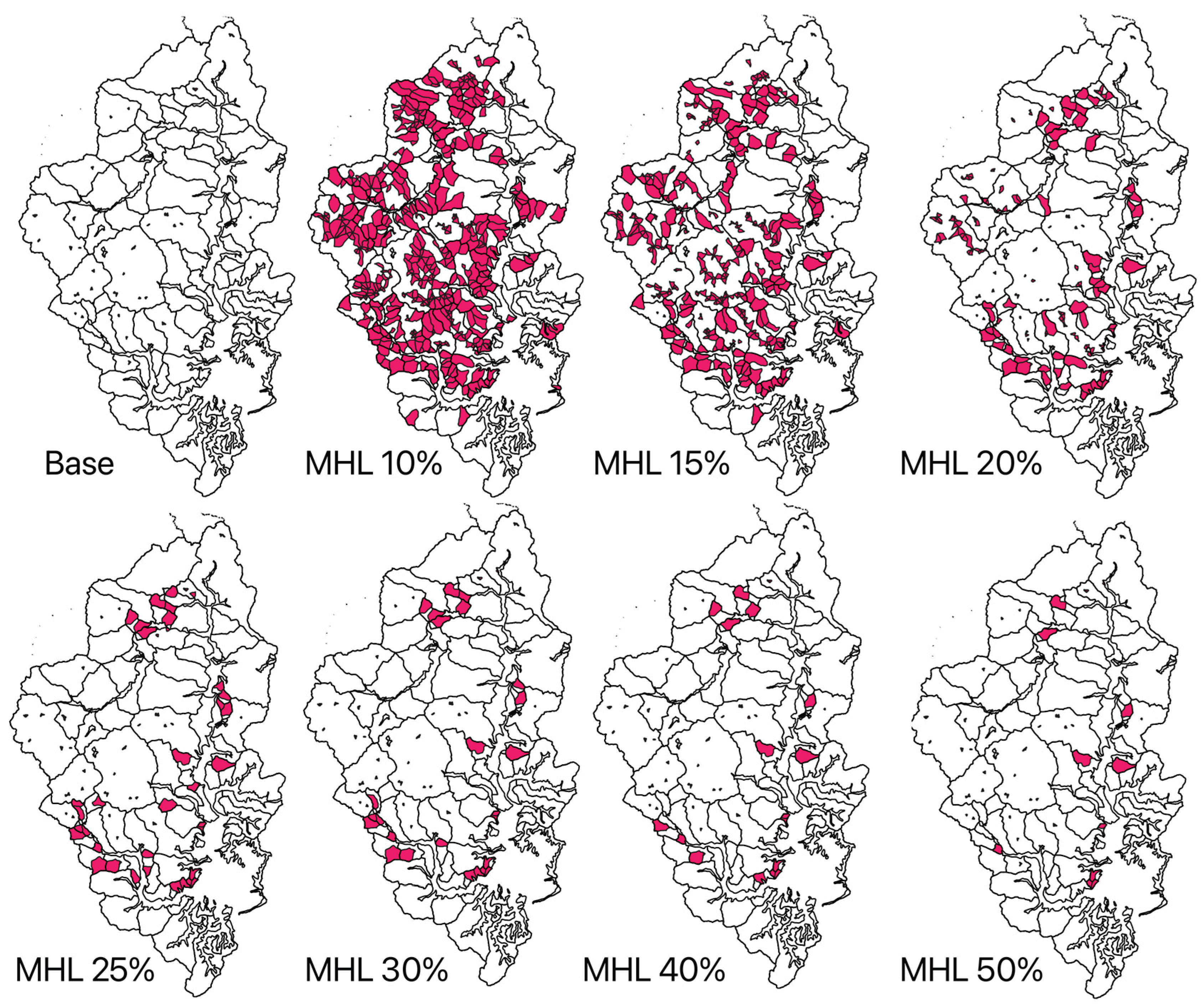
Figure 10.
The best solution considering an MHL of 25%, non-declining yield and non-declining RIL susceptibility constraints. The binary (1 = harvested, 0 = unharvested) solution was relaxed for those units in yellow in (a), meaning that fractions of those units will be harvested over several periods. Numbers in the bottom left side of each map represent the period in which the units were harvested.
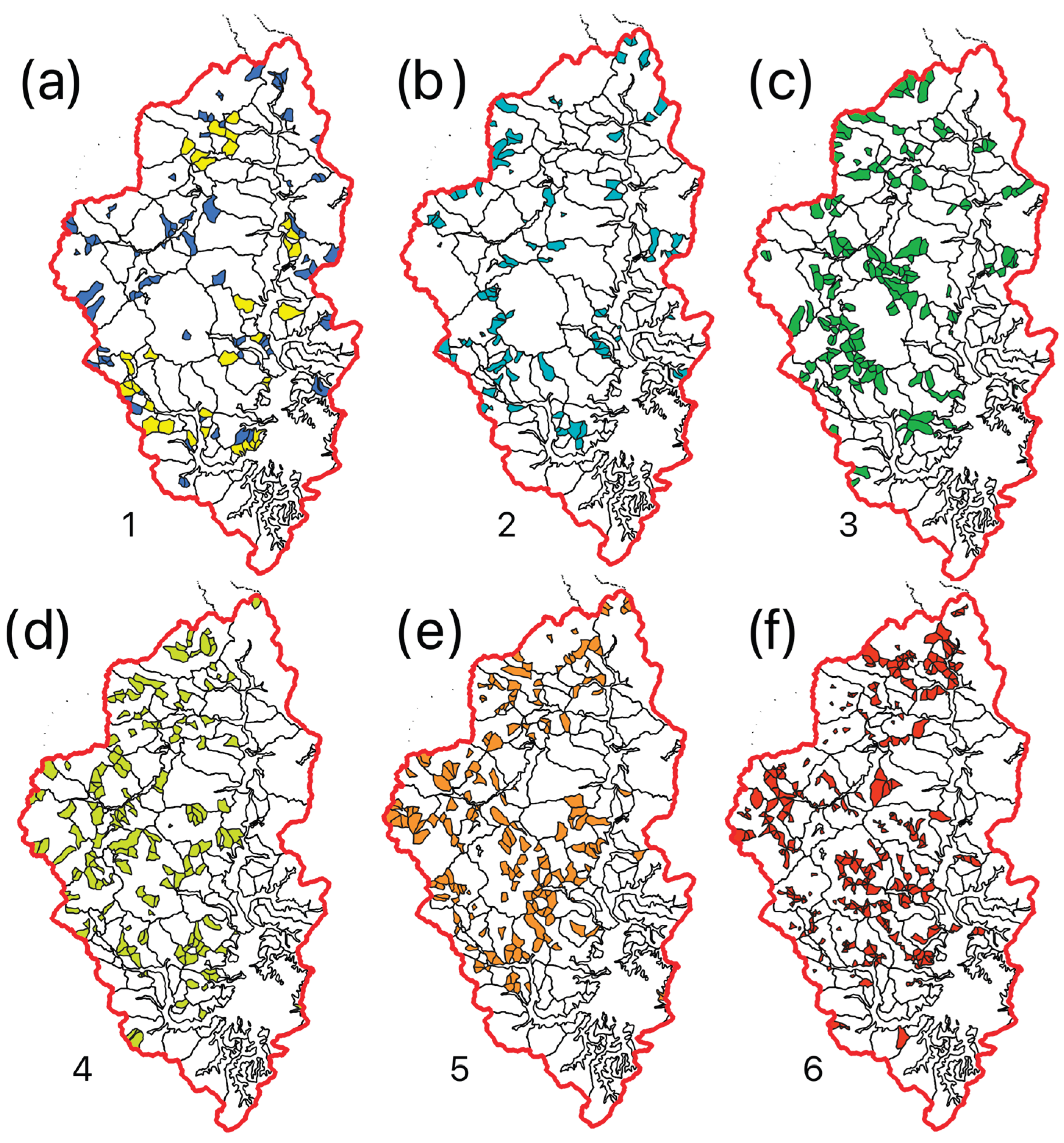

Table 1.
Variation in the percentage area by slope category (%) for the whole Uawa Catchment and forest plantations.
Table 1.
Variation in the percentage area by slope category (%) for the whole Uawa Catchment and forest plantations.
| Property | Slope (%) | |||||
| <14% | 14%–30% | 30%–40% | 40%–60% | 60%–80% | >80% | |
| Uawa Catchment | 19% | 27% | 21% | 24% | 7% | 2% |
| Forest Plantations | 6% | 26% | 26% | 33% | 8% | 1% |
Table 2.
Definition of fluvial system zones.
| Network position |
Stream Order |
Channel Gradient | Landforms | Dominant process |
| Zone 1 | 1,2 | High/steep | Headwater streams | Erosion |
| Zone 2 | 3,4 | Mid gradient | Pool/riffle, tributaries | Transfer/storage |
| Zone 3 | 5,6,7 | Low gradient | Main stem, floodplains | Deposition |
Table 3.
Summary of silvicultural, management and harvesting costs and the year in which they occurred. All costs are given in New Zealand dollars (NZD). Costs followed by the asterisk (*) only occur in the year shown.
Table 3.
Summary of silvicultural, management and harvesting costs and the year in which they occurred. All costs are given in New Zealand dollars (NZD). Costs followed by the asterisk (*) only occur in the year shown.
| Item | Cost (NZD/ha) | Year |
| Land cost | 10,000 | 0 *, 30 |
| Land prep, silvicultural costs | ||
| Tracking, land preparation | 100 | Year established |
| Pre-plant spray | 184 | 0 * |
| Seedlings, planting | 1300 | 0 * |
| Release spraying | 400 | 0 * |
| Mapping | 50 | 0 * |
| Thinning to waste | 900 | 4,8 |
| Annual costs | ||
| Forest Management | 40 | annually |
| Rates, insurance, administration | 42 | annually |
| Cost (NZD/m3) | Year | |
| Harvesting costs | ||
| Harvesting | VCM model | Year of harvest |
| Roading | VCM model | Year of harvest |
| Cartage | 19 | Year of harvest |
| Cost (NZD/km) | Year | |
| Road Construction | ||
| Primary roads | 137,091 | Year of harvest |
| Secondary roads and skid tracks | VCM model | Year of harvest |
Table 3.
Relevant metrics for the best catchment-oriented harvest schedule for the Uawa Catchment.
| 1 | 2 | 3 | 4 | 5 | 6 | ||
| Area Harvested | (ha) | 2788 | 3440 | 6894 | 6538 | 6122 | 5963 |
| Volume Harvested | (m3 / period) | 1905673 | 1906283 | 3521600 | 3949155 | 4220694 | 4282444 |
| Net Income | (NZD x 103) | 166,344 | 158,095 | 285,729 | 322,543 | 341,337 | 313,532 |
| Aggregated RIL susceptibility | 1553 | 1769 | 3618 | 3618 | 3618 | 3618 | |
| CMU proportion being harvested each period | Min | 0 | 0 | 0 | 0 | 0 | 0 |
| Mean | 0.0948 | 0.13 | 0.173 | 0.191 | 0.169 | 0.130 | |
| Max | 0.25 | 0.25 | 0.25 | 0.25 | 0.25 | 0.25 |
Table 4.
Areas harvested and remaining by age classes and periods along the planning horizon.
| Cut (ha) in class: | Volume harvested per period | |||||||||||
| Year | 0-5 | 5-10 | 10-15 | 15-20 | 20-25 | 25-30 | 30-35 | 35-40 | 40-45 | 45+ | (m3) | |
| 5 | 205 | 218 | 1420 | 571 | 375 | 0 | 1,905,673 | |||||
| 10 | 1371 | 1201 | 195 | 435 | 110 | 129 | 1,906,283 | |||||
| 15 | 2207 | 4368 | 96 | 4 | 4 | 215 | 3,521,600 | |||||
| 20 | 660 | 4413 | 1376 | 88 | 0 | 0 | 3,949,155 | |||||
| 25 | 13 | 1808 | 3995 | 301 | 5 | 0 | 4,220,694 | |||||
| 30 | 0 | 627 | 3096 | 2022 | 197 | 21 | 4,282,444 | |||||
| Stock (ha) in class: | Total Area | |||||||||||
| Year | 0-5 | 5-10 | 10-15 | 15-20 | 20-25 | 25-30 | 30-35 | 35-40 | 40-45 | 45+ | (ha) | |
| 0 | 648 | 5638 | 12684 | 7629 | 1601 | 419 | 1874 | 870 | 536 | 0 | 31,899 | |
| 5 | 2788 | 648 | 5638 | 12684 | 7629 | 1396 | 201 | 454 | 299 | 161 | 31,899 | |
| 10 | 3440 | 2788 | 648 | 5638 | 12684 | 6258 | 196 | 6 | 19 | 222 | 31,899 | |
| 15 | 6894 | 3440 | 2788 | 648 | 5638 | 10477 | 1890 | 100 | 2 | 22 | 31,899 | |
| 20 | 6538 | 6894 | 3440 | 2788 | 648 | 4978 | 6064 | 514 | 12 | 24 | 31,899 | |
| 25 | 6122 | 6538 | 6894 | 3440 | 2788 | 635 | 3170 | 2068 | 213 | 31 | 31,899 | |
| 30 | 5963 | 6122 | 6538 | 6894 | 3440 | 2788 | 8 | 74 | 47 | 26 | 31,899 | |
Disclaimer/Publisher’s Note: The statements, opinions and data contained in all publications are solely those of the individual author(s) and contributor(s) and not of MDPI and/or the editor(s). MDPI and/or the editor(s) disclaim responsibility for any injury to people or property resulting from any ideas, methods, instructions or products referred to in the content. |
© 2025 by the authors. Licensee MDPI, Basel, Switzerland. This article is an open access article distributed under the terms and conditions of the Creative Commons Attribution (CC BY) license (http://creativecommons.org/licenses/by/4.0/).
Copyright: This open access article is published under a Creative Commons CC BY 4.0 license, which permit the free download, distribution, and reuse, provided that the author and preprint are cited in any reuse.


