Submitted:
08 December 2025
Posted:
09 December 2025
You are already at the latest version
Abstract
This work presents a discrete theoretical model in which basal metabolic rate B is described as a dynamic function of an organism’s ontogenetic stage n. Instead of treating B only as a static function of body mass M, we adopt the form B(n) = B0 Mb(n), in which the effective scaling exponent b(n) varies systematically throughout development. In contrast to classical approaches, such as Kleiber’s empirical law (B ∝ M3/4) and the continuous fractal model of West–Brown–Enquist (WBE), which assume a constant exponent, the present framework emphasizes how the metabolic scaling relationship itself can evolve over the life cycle of a single individual. The model is inspired by a Fibonacci-based description of growth in discrete stages, leading to analytic expressions for b(n) that connect ontogenetic progression to changes in the scaling between metabolism and mass. In this setting, Kleiber’s constant B0 ≈ 70 kcal/day is reinterpreted as a metabolic anchoring point, linking the classical law B ≈ 70 M3/4 to a developmentally explicit formulation. We show that the resulting trajectory B(n) captures, at a conceptual level, how metabolic scaling can shift from strongly sublinear behavior at early stages towards an almost linear regime as n increases, and that the predicted basal rates remain compatible, in order of magnitude, with values reported for mammals of different sizes. In this way, the work offers a unified framework that connects the evolution of B(n) across ontogeny to the recursive organization of biological growth.
Keywords:
metabolic scaling
; biological development phases
; metabolic rate
; exponent based on Fibonacci
1. Introduction
The metabolic rate is, in essence, the "pace of life" of an animal, the speed at which its body converts food into energy to sustain all vital functions, from the beating of the heart to the movement of the muscles. This pace is not the same for all organisms; it varies in fascinating ways, influenced by factors such as body size, ambient temperature, and lifestyle. While a giant whale burns energy slowly and steadily, a hummingbird in frantic flight has an extremely accelerated metabolic "engine", requiring a constant intake of food. This relationship between body size and energetic expenditure, classically described by Kleiber [1], allows us to uncover how animals adapt to different environments and how they balance the delicate budget between the energy they obtain and the energy they spend simply to exist.
Kleiber’s Law [1] establishes the relationship between basal metabolic rate B and body mass M in animals in the form , and emerged from a methodological analysis that synthesized experimental data from multiple sources [2]. Max Kleiber compiled precise measurements of oxygen consumption (obtained by indirect calorimetry under basal conditions) in mammals spanning a wide range of body masses, from small rodents to cattle and elephants. When he attempted to relate mass and metabolism directly in a standard linear plot, the data produced a curve that was difficult to interpret, with values for small animals clustered at one end and values for large animals spread out at the other. The key to revealing the underlying pattern was to represent the data on a log–log plot, graphing as a function of . In this representation, the previously scattered experimental points aligned approximately along a straight line. This alignment is the mathematical signature of a power-law (or scaling law) of the form
where B represents the basal metabolic rate of the animal, M is its total body mass, a is a proportionality constant that indicates the level of metabolic rate for a unit mass (for example, 1 kg), and b is the scaling exponent, the central parameter of the law. Kleiber applied linear regression analysis to determine the slope of the best-fit line. This slope, denoted by b in the logarithmic equation , corresponds exactly to the scaling exponent in the original power-law relation (Eq. 1). The value Kleiber found for this slope was approximately , which became known as the three-quarter law. From the linear fit in logarithmic scale, Kleiber was able to determine not only the scaling exponent , but also the point at which this line crosses the vertical axis. This intercept, when converted back from the logarithmic scale to the arithmetic scale, corresponds to a value of approximately 70. Thus, the general expression of Kleiber’s Law, derived directly from his empirical analysis for mammals, can be written in a more complete form as
where B is the basal metabolic rate (in kcalday−1) and M is the body mass (in kg).
This expression tells us that, on average, each kilogram of a mammal does not "consume" metabolically in strict proportion to its mass, but according to the three-quarter power law. For example, to estimate the basal metabolism of a 20 kg dog, we apply kcal/day. Therefore, Kleiber’s analysis provided not only the scaling law (the exponent ), but also the scaling factor (), which turned an abstract mathematical relationship into a concrete predictive tool for comparative physiology. It is important to note that the exact value of a may vary slightly depending on the dataset or taxonomic group, but the exponent was, at the time, regarded by Kleiber as approximately universal among mammals.
While Kleiber’s work established that metabolism scales with mass raised to the power through statistical analysis of experimental data, it was the Metabolic Theory of West, Brown and Enquist [3] (WBE), formulated at the end of the same century, that set out to explain why this specific exponent emerges. The WBE model is based on a fundamental physical principle: the need to optimize the distribution of resources (such as nutrients and oxygen) throughout the body of an organism via hierarchical transport networks with fractal properties, such as the circulatory and respiratory systems. The theory argues that, to efficiently supply every cell in a three-dimensional body from a single source (such as the heart or lungs), the architecture of these networks must obey certain principles of scale invariance and space filling. The mathematical solution of this optimization problem, taking into account the fractal geometry of the networks, leads to a theoretical scaling exponent of . In this way, the WBE model offers a mechanistic and theoretical explanation for the empirical regularity discovered by Kleiber.
Both Kleiber’s empirical law and the theoretical model of West, Brown and Enquist (WBE) represent fundamental advances in describing metabolic scaling in adult organisms. In their classical formulations, both approaches treat the scaling exponent as a fixed, asymptotic value, characteristic of a "fully developed" organism. This assumption, however, shows limitations when confronted with empirical data for organisms undergoing growth. During ontogenetic development, from juvenile stages to maturity, systematic deviations from the three-quarter law are observed, since the effective metabolic exponent is not constant and varies in a predictable way over time. Although the conceptual framework of WBE has been extended to describe ontogenetic growth, it still generally assumes a constant metabolic exponent. Thus, both Kleiber’s analysis and the WBE model, by focusing primarily on the relationship between adult individuals of different sizes (an interspecific approach), do not explicitly incorporate the possibility of a dynamic exponent along the life cycle of a single individual. In this respect, these classical models do not fully capture the dynamics of intraspecific scaling during development, leaving a gap precisely in the stages where energy allocation to the construction of new structures (biosynthesis) directly competes with the maintenance of basal functions.
In this context arises the need for models that describe the metabolic exponent b not as a universal constant, but as a variable function of the organism’s developmental stage n. This limitation of classical models is supported by a growing body of literature documenting variation in the metabolic scaling exponent under different conditions. Glazier shows that the supposed universality of the three-quarter law does not hold either among or within species, with exponents that vary consistently as a function of ontogenetic, ecological and physiological factors [4,5]. This suggests that a more comprehensive theory of metabolic scaling must incorporate the dynamic nature of the exponent b during ontogenetic growth, reconciling changes in the organism’s energetic priorities with the deviations observed from the three-quarter law.
A previous formulation of the Fibonacci-based ontogenetic model, focusing on the estimation of and on the quantitative comparison with empirical metabolic data, was presented in Cambui (2025) [6]. In the present work, we adopt a complementary perspective: we emphasize the didactic derivation of the expressions for and for the metabolic rate , as well as the conceptual interpretation of the ontogenetic dynamics predicted by the model.
In light of this evidence, it becomes natural to seek a theoretical framework in which the metabolic exponent b can, in fact, vary throughout development. Building on the discussion above, we propose a discrete model in which metabolic activity emerges from an intrinsic developmental programming logic. In this model, the regulation of metabolism over growth is not described as a continuous and homogeneous process, but as a sequence of successive, discrete stages. At each stage n, the organism reorganizes its energetic priorities (for example, between biosynthesis and maintenance), which is reflected in a distinct effective value for the exponent . In this way, ontogenetic progression is understood as a succession of metabolically programmed phases, providing a formal structure capable of explicitly accommodating the variation of the exponent b as a function of the developmental stage n.
The model in a nutshell:
- Organisms do not only differ in size; they also pass through identifiable developmental stages (e.g., infant, juvenile, adult).
- We propose that the metabolic scaling exponent b is not fixed, but changes with each developmental stage n.
- This change follows a discrete pattern inspired by the Fibonacci sequence, often used to model stepwise growth in nature.
- The result is a dynamic scaling law,in which both M and are interpreted in relation to the organism’s stage of growth.
- Kleiber’s static law appears as a special case within this more general, stage-dependent framework, for stages (or species) in which .
2. From Recursive Growth to Metabolic Scaling
Before proceeding, it is important to clarify how the present section relates to our earlier work. A formal derivation of the Fibonacci-based ontogenetic model, including the construction of the recursive growth scheme and the analytical expression for the exponent , was already presented in Cambui (2025) [6], with emphasis on parameter estimation and quantitative comparison with empirical data. Here, we revisit the same mathematical backbone with a different purpose: to reorganize the derivation in a more didactic way and to make explicit how the recursive growth hypothesis leads naturally to a stage-dependent metabolic law of the form . The focus is therefore not on proposing a new model, but on clarifying the logical steps that connect recursive mass growth to metabolic scaling.
Based on the recursive property of the Fibonacci sequence, expressed by , we propose a biological analogy. If we imagine that the growth of an organism is not continuous, but occurs in discrete, successive stages (such as juvenile and adult phases), in which the mass acquired at each new stage depends on the gains from the two previous stages, we can transpose this mathematical logic to body mass. This leads to a similar recursive relation for the mass at each stage n: . Solving this recurrence, as is done for the Fibonacci sequence, we obtain that the total mass after n stages grows approximately exponentially, following
where is the Golden Ratio.
At first sight, the expression may seem like a bold or even controversial simplification, since it models the growth of the mass of a complex organism using an exponential formula based on the Golden Ratio, a pattern more frequently associated with static forms than with dynamic processes. However, its value lies less in being a literal and precise description of every gram of tissue, and more in functioning as a minimal conceptual model. It captures the central idea that growth occurs in discrete stages n, in which each new step amplifies the existing mass by an approximately constant factor related to . Solving Eq. (2) for n, we arrive at
which opens the way to relate this stage n to metabolic rate.
The growth stage n allows a fundamental reformulation of the relationship between metabolism and mass. Instead of treating metabolic rate as a static function of mass, we can express it as a dynamic function of the developmental stage:
in which the scaling exponent is no longer a constant and now depends explicitly on the ontogenetic stage. This formulation establishes a crucial distinction with respect to the classical law . In the classical view, the exponent b is a fixed value, such as Kleiber’s , which describes an average relationship among adult individuals of different sizes, and mass M plays the role of the only independent variable. In contrast, in the expression , the exponent becomes a variable that depends on the developmental stage. This means that, for a single individual, the rule that relates metabolism and mass changes systematically throughout its growth, from the initial stages of rapid mass gain to maturity. While the classical law answers the question “how does an adult elephant differ from an adult rat?”, the new formulation seeks to answer “how do the efficiency and metabolic priorities of an organism change as it grows?”. In this way, the introduction of the stage n and of the variable exponent represents a shift from a comparative, static model to a dynamic model that aims to capture the ontogenetic trajectory of metabolism over the life cycle of an individual.
In our model, we propose a mathematical idealization in which the total body mass of an organism at developmental stage n, denoted by , grows in proportion to the corresponding term of the Fibonacci sequence, so that (I). This choice reflects the idea that biological growth often proceeds in discrete steps, in which each new stage incorporates and adds to the structures established in previous stages.
This also captures an important physiological principle: established tissues, even when they are not at maximal functional activity — such as a skeletal muscle at rest, which is not actively contracting, or hepatic parenchyma between detoxification cycles — still require energy to maintain cellular integrity, membrane potential, and routine protein synthesis. This continuous expenditure, essential for maintaining homeostasis and physiological readiness, constitutes the basal maintenance cost. Thus, we have (II).
Starting from the general expression for metabolic scaling, (Eq. 4), we can isolate the stage-dependent scaling exponent, obtaining
Substituting relations (I) and (II) into Eq. (5), we arrive at an expression that links the exponent directly to the ratio between consecutive Fibonacci terms:
The Fibonacci sequence has a well-known asymptotic form, given by
and therefore the ratio between consecutive terms satisfies
Inserting the approximations (7) and (8) into Eq. (6) and applying logarithmic properties, we obtain the refined form of the exponent:
For organisms at advanced developmental stages, where n takes large values, the constant term becomes negligible compared to . In this limit, the expression simplifies significantly to
3. Dynamics of the Scaling Exponent as a Function of Stage n
To illustrate how the metabolic exponent varies throughout development, we apply the model formulas directly, in both the simplified and refined versions, to the first ten stages. Table 1 compares the values of and , which includes the correction term . This comparison is particularly useful, as it allows us to check the internal consistency of the model, identify from which point the two formulations begin to agree approximately, and, most importantly, observe the trajectory traced by the exponent, from the more sensitive initial stages to more advanced phases in which a clear pattern emerges.
The analysis of the values in Table 1 reveals three important behaviors that characterize and qualify our Fibonacci-based growth model.
First, we observe that for the earliest developmental stages (especially for ), the refined model, which takes into account the constant term , yields values of that fluctuate dramatically, even reaching a negative result for . This indicates that the more detailed formulation requires interpretative caution in this initial range. Such fluctuations reflect the sensitivity of the model to the initial mass and to the transition between the first terms of the sequence, which have not yet entered the asymptotic regime. In biological practice, this initial phase may be associated with embryonic or larval stages, in which the relationship between mass and metabolism is highly dynamic and influenced by specific factors that go beyond a simple scaling pattern, so that the model should be viewed there only as a qualitative heuristic.
Second, starting from , the values of the two versions begin to converge rapidly. The refined exponent stabilizes and begins to closely follow the trajectory of the simplified version. This indicates that, after the first critical stages, the constant term loses influence and the behavior of the model is dominated by the underlying recursive logic.
Finally, and most significantly, both curves display a clear and consistent trend: as n increases, the exponent approaches 1 asymptotically. In the theoretical limit , this corresponds to a regime in which metabolism tends to scale approximately linearly with mass (). For intermediate stages, the values of pass through the biologically relevant sublinear range (for example, between and ), suggesting a possible ontogenetic transition: while young, rapidly growing organisms operate under a stronger efficiency constraint (more pronounced sublinear scaling), more mature organisms approach a regime in which the metabolic cost becomes progressively more proportional to their total mass.
4. Kleiber’s Law as a Metabolic Anchoring Point
Having established the functional form of the exponent along development, we can now place Kleiber’s law within this new ontogenetic framework.
From the standpoint of the proposed model, the metabolic rate thus acquires a dynamic expression that integrates both the universality observed by Kleiber and the variable nature of ontogenetic growth. Starting from the general form
we can reinterpret the meaning of Kleiber’s intercept a. In his classical law, , the constant 70 (in kcal/day) represents the expected basal metabolic cost for a hypothetical adult mammal of 1 kg. In our model, this reference value is not discarded; instead, it acts as a metabolic anchoring point that sets the energetic scale, while the developmental dynamics are captured by the variation of the exponent .
In this way, the expression for the metabolic rate at stage n can be written as
where M is the total body mass of the organism at that specific stage, and is given by Eqs. (9) and (10), depending on whether one wishes to consider the refined correction or the asymptotic limit. This formulation reveals the following dependence: mass M sets the overall scale of the organism, but the scaling rule is modulated by the developmental stage n, which in turn is linked to mass through the approximate relation
Consequently, the model not only recovers Kleiber’s law as an approximate case, that is, for certain stages in which , but also provides a framework to systematically describe deviations from this value during growth. In early ontogenetic stages, the model predicts lower values of , which implies a metabolic rate below that predicted by the three-quarter law for a given mass M, reflecting a more strongly sublinear scaling regime. As n increases, the exponent grows and, in the theoretical limit of very advanced stages, tends to 1, bringing metabolism closer to an almost linear relationship with mass. Thus, Kleiber’s intercept remains a fundamental physiological landmark on the energetic scale, while the function introduces the temporal and developmental dimension that was missing, linking the comparative perspective among species with the dynamic trajectory of each individual over its life cycle.
5. Ontogenetic Results for the Metabolic Rate in Mammals
Although in previous work, already accepted for publication, we have demonstrated the predictive capacity of the model by computing the exponents for specific species and comparing them with an extensive compilation of empirical data [6], the present article adopts a distinct and complementary focus. Here, our goal is to explore the theoretical implications of the model in a more discursive and didactic way, detailing step by step the derivation of the equations that culminate in the central expression .
We concentrate on analyzing the behavior of this function and the biological interpretation of its dynamics, in particular how the variation of the exponent modulates the relationship between mass and metabolism throughout development. When appropriate, we make qualitative comparisons with general trends reported in the literature, illustrating how the theoretical trajectory of connects with known physiological patterns, without the need for a new exhaustive statistical analysis. In this way, the text aims to consolidate the theoretical foundations of the model and expand its conceptual discussion, establishing a clear bridge between the proposed mathematical structure and the principles of developmental physiology.
Table 2 brings together, in a single panel, the main quantities of the model for different mammalian species. The first column indicates the species; the second shows the body mass interval M considered in each case. The next two columns show the intervals of the scaling exponent obtained in our previous work, in the simplified version and in the refined version . The following column displays the reference metabolic rate , computed from the classical Kleiber law . Finally, the last two columns present the basal metabolic rate intervals predicted by the ontogenetic model, and , calculated from the relation . In this way, the table allows one to visualize simultaneously how mass, exponent, and metabolic rate are organized into different ranges across body size, with Kleiber’s law serving as a comparative reference.
Some general patterns emerge clearly. First, all exponents remain in the sublinear regime, with typical values between and , in agreement with the literature on metabolic scaling in mammals. Moreover, for each species, the refined version is systematically smaller than the simplified version , reflecting the influence of the corrective term present in the full expression of the exponent. This difference is small for small and medium-sized species (for example, rat, rabbit, cat, and dog), but becomes progressively more relevant for large species (horse, cow, elephant, and blue whale).
This behavior translates directly into the intervals of B. For small and intermediate mammals, the ranges of and are close to each other and also comparable, in order of magnitude, to the reference rate . This indicates that, in these cases, the asymptotic approximation already captures the dependence between mass and metabolism satisfactorily, and that the ontogenetic model reproduces, in a qualitative sense, the predictions of Kleiber’s law. In contrast, for large mammals, the intervals based on are noticeably smaller than those obtained with and lie closer to , revealing an attenuation of the sensitivity of to mass when the logarithmic correction is taken into account. In biological terms, this means that the refined version avoids overestimating the daily energetic cost of very heavy organisms, yielding predictions more consistent with the idea that metabolic scaling becomes less steep at high body masses.
In summary, Table 2 shows that the model generates plausible metabolic rate intervals across several orders of magnitude in body mass and is consistently aligned with Kleiber’s law, which here plays the role of a classical baseline. At the same time, the table highlights the conceptual role of the two versions of the exponent: the simplified form offers a compact and intuitive description of the asymptotic behavior, whereas the refined form introduces an essential correction to more realistically represent the metabolism of large species, bringing its predictions closer to the rates expected from classical scaling.
Finally, we would like to make explicit our perspective on the equation , the core of this model. We are aware that proposing that the mass growth of a complex organism follows a geometric progression based on the golden ratio is a strong and, at first glance, controversial hypothesis. Our defense of this postulate, however, is not that it faithfully describes the mass at every instant of development, but rather that it captures, in a synthetic way, the structural logic of growth organized into discrete stages, in which each step amplifies the previous one by an approximately constant factor. Within the aims of this work, we did not identify an equally simple alternative and, in a certain sense, we had no conceptual choice that would simultaneously preserve stepwise recursion, the link with the Fibonacci sequence, and the possibility of obtaining an analytical expression for and, consequently, for . We therefore view the relation as a powerful heuristic tool: a deliberately radical simplification that, by isolating the principle of recursion in stages, makes visible dynamic relationships that more continuous and realistic models tend to conceal. The controversy associated with this choice is not regarded here as a flaw, but as an invitation to dialogue and to a critical exploration of the extent to which fundamental mathematical principles, such as those encoded in the Fibonacci sequence and in the golden ratio, may manifest themselves in the architecture of biological growth.
Figure 1 illustrates, in a simple way, how the metabolic rate evolves along developmental stages in the context of the proposed model. For purely illustrative purposes, we assume a mass that grows as (with ), so as to emphasize the role of the dynamic exponent in the expression . The solid curve shows the values obtained with the simplified version of the exponent, , whereas the dashed curve corresponds to the refined version .
Several important aspects can be observed. First, both curves describe a monotonic increase of with developmental stage, reflecting the fact that more developed organisms, with larger mass, require more energy to sustain their vital functions. Second, the difference between the two versions is more evident in the early stages, when the corrective term in the refined expression still exerts a significant influence on . From onward, the two trajectories become very close, indicating that, as development progresses, the asymptotic form already captures well the essential dynamics of the model. Thus, the figure serves as a visual “proof of concept”: it shows how, even in a simplified scenario, the combination of stage-structured growth with a variable scaling exponent produces a metabolic trajectory that increases and is consistent with the idea of a scaling that becomes progressively less sublinear along development.
Conclusion
This work started from a simple yet fundamental observation: organisms are not static, they grow and develop. Classical laws of metabolic scaling, such as Kleiber’s law and the WBE theory, were essential to describe how much the metabolism of an adult elephant differs from that of an adult rat, but they showed limitations in explaining how the metabolism of a single individual changes over the course of its own life, from the juvenile phase to maturity.
To address this gap, we proposed a change in perspective. Instead of seeking a single fixed exponent that describes all organisms, we developed a model in which the scaling exponent "grows" together with the organism. Inspired by stage-like growth patterns, so common in nature and mathematically described by the Fibonacci sequence, we structured development as a succession of discrete stages. In this view, the relationship between mass and metabolism is no longer governed by an immutable rule, but is described by a dynamic power law,
in which the exponent varies systematically with the ontogenetic stage n.
The main outcome of this framework is the description of a metabolic trajectory along development. The model predicts that, in early stages, energy expenditure scales with mass more gently (lower exponent), which is consistent with the idea that, in these phases, a large fraction of the energy budget is associated with the construction and reorganization of tissues. As the organism matures, the relationship between B and M becomes progressively more direct, with approaching higher values and, in the limit, a nearly linear regime. In this way, the dynamics of allow ontogenetic development to be incorporated into scaling theory, using Kleiber’s classical value as a metabolic anchoring reference.
Ultimately, this work does not discard the achievements of previous theories, but places them in a broader and more dynamic context. By translating the recursive logic of Fibonacci into the language of physiology, we offer an alternative and complementary narrative for the phenomenon of scaling, intrinsically linked to time and to the process of becoming a complete organism. This theoretical framework, centered on principles of stepwise organization, opens the way for future investigations into how life history, energetic priorities at each phase, and the very hierarchical architecture of living beings intertwine to define the pace of life, and how these ideas can be systematically confronted with metabolic data across development.
References
- Kleiber, M. Body size and metabolism. Hilgardia 1932, 6(11), 315. [Google Scholar] [CrossRef]
- Savage, V. M.; Gillooly, J. F.; Woodruff, W. H.; West, G. B.; Allen, A. P.; Enquist, B. J.; Brown, J. H. The predominance of quarter-power scaling in biology. Functional Ecology 2004, 18(2), 257. [Google Scholar] [CrossRef]
- West, G. B.; Brown, J. H.; Enquist, B. J. A general model for the origin of allometric scaling laws in biology. Science 1997, 276, 122. [Google Scholar] [CrossRef] [PubMed]
- Glazier, D. S. Beyond the 3/4-power law: variation in the intra- and interspecific scaling of metabolic rate in animals. Biological Reviews 2005, 80, 611. [Google Scholar] [CrossRef] [PubMed]
- Glazier, D. S. A unifying explanation for diverse metabolic scaling in animals and plants. Biological Reviews 2010, 85, 111. [Google Scholar] [CrossRef] [PubMed]
- Cambui, D. S. Metabolic scaling from Fibonacci dynamics. bioRxiv Also available as;[physics.bio-ph. 2025. [Google Scholar] [CrossRef]
Figure 1.
Example of the metabolic rate computed from for , assuming and using the simplified and refined versions of . The plot illustrates how the choice between the simplified and refined exponent affects the predicted metabolic trajectory, particularly in early developmental stages.
Figure 1.
Example of the metabolic rate computed from for , assuming and using the simplified and refined versions of . The plot illustrates how the choice between the simplified and refined exponent affects the predicted metabolic trajectory, particularly in early developmental stages.
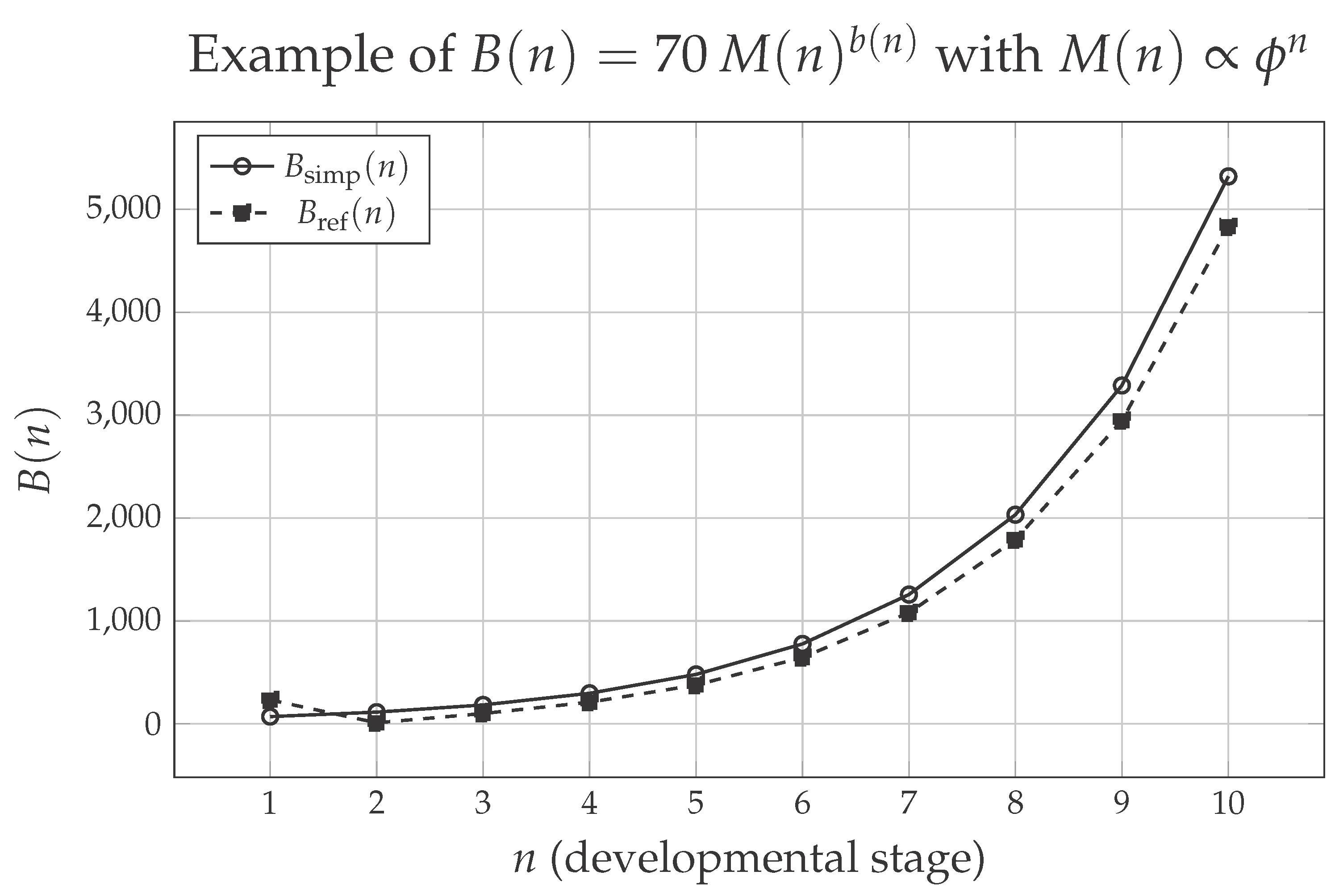

Table 1.
Values of the simplified exponent and of the refined exponent as a function of the developmental stage n.
Table 1.
Values of the simplified exponent and of the refined exponent as a function of the developmental stage n.
| n | ||||||||||
|---|---|---|---|---|---|---|---|---|---|---|
| 1.0000 | 2.0000 | 3.0000 | 4.0000 | 5.0000 | 6.0000 | 7.0000 | 8.0000 | 9.0000 | 10.0000 | |
| 0.0000 | 0.5000 | 0.6670 | 0.7500 | 0.8000 | 0.8330 | 0.8570 | 0.8750 | 0.8890 | 0.9000 | |
| 2.4880 | -2.0510 | 0.2470 | 0.5700 | 0.7000 | 0.7690 | 0.8120 | 0.8420 | 0.8640 | 0.8800 | |
Table 2.
Body mass intervals M, scaling exponents (simplified and refined versions), and metabolic rates predicted by the Kleiber and ontogenetic models for different mammalian species. Metabolic rates are in kcal/day.
Table 2.
Body mass intervals M, scaling exponents (simplified and refined versions), and metabolic rates predicted by the Kleiber and ontogenetic models for different mammalian species. Metabolic rates are in kcal/day.
| Species | M (kg) | |||||
|---|---|---|---|---|---|---|
| Rabbit | ||||||
| Rat | ||||||
| Mouse | ||||||
| Cat | ||||||
| Dog (medium) | ||||||
| Horse | ||||||
| Cow | ||||||
| Elephant | ||||||
| Blue Whale |
Disclaimer/Publisher’s Note: The statements, opinions and data contained in all publications are solely those of the individual author(s) and contributor(s) and not of MDPI and/or the editor(s). MDPI and/or the editor(s) disclaim responsibility for any injury to people or property resulting from any ideas, methods, instructions or products referred to in the content. |
© 2025 by the authors. Licensee MDPI, Basel, Switzerland. This article is an open access article distributed under the terms and conditions of the Creative Commons Attribution (CC BY) license (http://creativecommons.org/licenses/by/4.0/).
Copyright: This open access article is published under a Creative Commons CC BY 4.0 license, which permit the free download, distribution, and reuse, provided that the author and preprint are cited in any reuse.


