A Novel Grouped-Gram-Based Algorithm for Fast and Memory-Efficient Fixed Effects Estimation

1. Introduction

Fixed effects models appear widely in empirical research. The standard approach applies the within transformation: subtract unit means from each observation and form cross-products from the transformed arrays. This is direct and compatible with linear algebra routines, yet the method reshapes the data and performs multiple passes across memory. These operations become costly once the panel grows large relative to cache or main memory bandwidth.

Grouped Gram representations avoid array centering by replacing the transformation with sufficient statistics. These statistics summarize each unit’s contribution with sums and cross-products. The result is mathematically identical to the classical estimator. The central distinction lies in the structure of the computation. Grouped summaries allow a single pass through the data while maintaining numerical precision.

The study draws on several literatures. Panel methods in econometrics provide the model foundations [1,9,12,19]. Matrix computation references outline the algebra of Gram matrices [3,6,7]. Work on cache behavior and communication bounds frames the memory analysis [5,8,11,18]. The bootstrap section relies on Cameron et al. [2], Davison Hinkley [4].

2. Setup and Notation

Units are indexed by $\mathrm{i}=1,\dots ,\mathrm{N}$ and periods by $\mathrm{t}=1,\dots ,{\mathrm{T}}_{\mathrm{i}}$. The model is

$${\mathrm{y}}_{\mathrm{i}\mathrm{t}}={\mathrm{x}}_{\mathrm{i}\mathrm{t}}^{\prime }\mathrm{\beta }+{\mathrm{\alpha }}_{\mathrm{i}}+{\mathrm{\epsilon }}_{\mathrm{i}\mathrm{t}},$$

(1)

with covariates ${\mathrm{x}}_{\mathrm{i}\mathrm{t}}\in {\mathbb{R}}^{\mathrm{p}}$, unknown coefficient vector $\mathrm{\beta }$, and unit fixed effects ${\mathrm{\alpha }}_{\mathrm{i}}$.

Define

$${\overline{\mathrm{x}}}_{\mathrm{i}}\stackrel{\mathrm{def}}{=}{\displaystyle \frac{1}{{\mathrm{T}}_{\mathrm{i}}}}\sum _{\mathrm{t}=1}^{{\mathrm{T}}_{\mathrm{i}}}{\mathrm{x}}_{\mathrm{i}\mathrm{t}},{\overline{\mathrm{y}}}_{\mathrm{i}}\stackrel{\mathrm{def}}{=}{\displaystyle \frac{1}{{\mathrm{T}}_{\mathrm{i}}}}\sum _{\mathrm{t}=1}^{{\mathrm{T}}_{\mathrm{i}}}{\mathrm{y}}_{\mathrm{i}\mathrm{t}}.$$

The within-transformed values are

$${\mathrm{x}}_{\mathrm{i}\mathrm{t}}^{*}={\mathrm{x}}_{\mathrm{i}\mathrm{t}}-{\overline{\mathrm{x}}}_{\mathrm{i}},{\mathrm{y}}_{\mathrm{i}\mathrm{t}}^{*}={\mathrm{y}}_{\mathrm{i}\mathrm{t}}-{\overline{\mathrm{y}}}_{\mathrm{i}}.$$

The estimator is

$${\widehat{\mathrm{\beta }}}_{\mathrm{within}}={\left(\sum _{\mathrm{i}=1}^{\mathrm{N}}\sum _{\mathrm{t}=1}^{{\mathrm{T}}_{\mathrm{i}}}{\mathrm{x}}_{\mathrm{i}\mathrm{t}}^{*}{\mathrm{x}}_{\mathrm{i}\mathrm{t}}^{*\prime }\right)}^{-1}\left(\sum _{\mathrm{i}=1}^{\mathrm{N}}\sum _{\mathrm{t}=1}^{{\mathrm{T}}_{\mathrm{i}}}{\mathrm{x}}_{\mathrm{i}\mathrm{t}}^{*}{\mathrm{y}}_{\mathrm{i}\mathrm{t}}^{*}\right).$$

(2)

3. Grouped Gram Representation

Let the grouped sums and cross-products be

$${\mathrm{s}}_{\mathrm{x},\mathrm{i}}=\sum _{\mathrm{t}=1}^{{\mathrm{T}}_{\mathrm{i}}}{\mathrm{x}}_{\mathrm{i}\mathrm{t}},{\mathrm{s}}_{\mathrm{y},\mathrm{i}}=\sum _{\mathrm{t}=1}^{{\mathrm{T}}_{\mathrm{i}}}{\mathrm{y}}_{\mathrm{i}\mathrm{t}},$$

$${\mathrm{G}}_{\mathrm{i}}=\sum _{\mathrm{t}=1}^{{\mathrm{T}}_{\mathrm{i}}}{\mathrm{x}}_{\mathrm{i}\mathrm{t}}{\mathrm{x}}_{\mathrm{i}\mathrm{t}}^{\prime },{\mathrm{g}}_{\mathrm{i}}=\sum _{\mathrm{t}=1}^{{\mathrm{T}}_{\mathrm{i}}}{\mathrm{x}}_{\mathrm{i}\mathrm{t}}{\mathrm{y}}_{\mathrm{i}\mathrm{t}}.$$

3.1. Derivation of Gram Identities

Write

$${\mathrm{x}}_{\mathrm{i}\mathrm{t}}^{*}={\mathrm{x}}_{\mathrm{i}\mathrm{t}}-{\displaystyle \frac{{\mathrm{s}}_{\mathrm{x},\mathrm{i}}}{{\mathrm{T}}_{\mathrm{i}}}}.$$

Then

$$\begin{array}{cc}\hfill \sum _{\mathrm{t}=1}^{{\mathrm{T}}_{\mathrm{i}}}{\mathrm{x}}_{\mathrm{i}\mathrm{t}}^{*}{\mathrm{x}}_{\mathrm{i}\mathrm{t}}^{*\prime }& =\sum _{\mathrm{t}=1}^{{\mathrm{T}}_{\mathrm{i}}}\left({\mathrm{x}}_{\mathrm{i}\mathrm{t}}-{\displaystyle \frac{{\mathrm{s}}_{\mathrm{x},\mathrm{i}}}{{\mathrm{T}}_{\mathrm{i}}}}\right){\left({\mathrm{x}}_{\mathrm{i}\mathrm{t}}-{\displaystyle \frac{{\mathrm{s}}_{\mathrm{x},\mathrm{i}}}{{\mathrm{T}}_{\mathrm{i}}}}\right)}^{\prime }\hfill \end{array}$$

(3)

$$\begin{array}{cc}\hfill & =\sum _{\mathrm{t}=1}^{{\mathrm{T}}_{\mathrm{i}}}{\mathrm{x}}_{\mathrm{i}\mathrm{t}}{\mathrm{x}}_{\mathrm{i}\mathrm{t}}^{\prime }-{\displaystyle \frac{{\mathrm{s}}_{\mathrm{x},\mathrm{i}}{\mathrm{s}}_{\mathrm{x},\mathrm{i}}^{\prime }}{{\mathrm{T}}_{\mathrm{i}}}}-{\displaystyle \frac{{\mathrm{s}}_{\mathrm{x},\mathrm{i}}{\mathrm{s}}_{\mathrm{x},\mathrm{i}}^{\prime }}{{\mathrm{T}}_{\mathrm{i}}}}+{\displaystyle \frac{{\mathrm{T}}_{\mathrm{i}}{\mathrm{s}}_{\mathrm{x},\mathrm{i}}{\mathrm{s}}_{\mathrm{x},\mathrm{i}}^{\prime }}{{\mathrm{T}}_{\mathrm{i}}^2}}.\hfill \end{array}$$

(4)

Since

$${\displaystyle \frac{{\mathrm{T}}_{\mathrm{i}}{\mathrm{s}}_{\mathrm{x},\mathrm{i}}{\mathrm{s}}_{\mathrm{x},\mathrm{i}}^{\prime }}{{\mathrm{T}}_{\mathrm{i}}^2}}={\displaystyle \frac{{\mathrm{s}}_{\mathrm{x},\mathrm{i}}{\mathrm{s}}_{\mathrm{x},\mathrm{i}}^{\prime }}{{\mathrm{T}}_{\mathrm{i}}}},$$

the terms combine to

$$\sum _{\mathrm{t}=1}^{{\mathrm{T}}_{\mathrm{i}}}{\mathrm{x}}_{\mathrm{i}\mathrm{t}}^{*}{\mathrm{x}}_{\mathrm{i}\mathrm{t}}^{*\prime }\equiv {\mathrm{G}}_{\mathrm{i}}-{\displaystyle \frac{{\mathrm{s}}_{\mathrm{x},\mathrm{i}}{\mathrm{s}}_{\mathrm{x},\mathrm{i}}^{\prime }}{{\mathrm{T}}_{\mathrm{i}}}}.$$

(5)

The same logic applies to the cross-product:

$$\sum _{\mathrm{t}=1}^{{\mathrm{T}}_{\mathrm{i}}}{\mathrm{x}}_{\mathrm{i}\mathrm{t}}^{*}{\mathrm{y}}_{\mathrm{i}\mathrm{t}}^{*}\equiv {\mathrm{g}}_{\mathrm{i}}-{\displaystyle \frac{{\mathrm{s}}_{\mathrm{x},\mathrm{i}}{\mathrm{s}}_{\mathrm{y},\mathrm{i}}}{{\mathrm{T}}_{\mathrm{i}}}}.$$

3.2. Estimator Based on Grouped Summaries

Summing across units yields the estimator

$${\widehat{\mathrm{\beta }}}_{\mathrm{fast}}={\left(\sum _{\mathrm{i}=1}^{\mathrm{N}}\left[{\mathrm{G}}_{\mathrm{i}}-{\displaystyle \frac{{\mathrm{s}}_{\mathrm{x},\mathrm{i}}{\mathrm{s}}_{\mathrm{x},\mathrm{i}}^{\prime }}{{\mathrm{T}}_{\mathrm{i}}}}\right]\right)}^{-1}\left(\sum _{\mathrm{i}=1}^{\mathrm{N}}\left[{\mathrm{g}}_{\mathrm{i}}-{\displaystyle \frac{{\mathrm{s}}_{\mathrm{x},\mathrm{i}}{\mathrm{s}}_{\mathrm{y},\mathrm{i}}}{{\mathrm{T}}_{\mathrm{i}}}}\right]\right),$$

(6)

which equals the within estimator in exact arithmetic.

4. Memory Path Differences

The within transformation forms ${\mathrm{x}}_{\mathrm{i}\mathrm{t}}^{*}$ and ${\mathrm{y}}_{\mathrm{i}\mathrm{t}}^{*}$ explicitly. Each assignment causes reads and writes across arrays of size $\mathrm{n}={\sum }_{\mathrm{i}}{\mathrm{T}}_{\mathrm{i}}$. Since modern processors face bandwidth limitations [8,14], these memory operations dominate the floating point operations once n is large.

The grouped estimator performs a single pass through the data. For each i, the algorithm accumulates ${\mathrm{s}}_{\mathrm{x},\mathrm{i}}$, ${\mathrm{s}}_{\mathrm{y},\mathrm{i}}$, ${\mathrm{G}}_{\mathrm{i}}$, and ${\mathrm{g}}_{\mathrm{i}}$. The cross-product corrections rely on these summaries alone. This reduces memory traffic by avoiding write-back of centered arrays.

The roofline model [18] frames the method: algorithms with high byte movement relative to floating point work fall below peak performance. Since the fast estimator avoids array writes, its arithmetic intensity improves.

Communication bounds [5,11] support this point. The within transformation moves $\mathrm{O}\left(\mathrm{n}\mathrm{p}\right)$ numbers, while the grouped approach touches each ${\mathrm{x}}_{\mathrm{i}\mathrm{t}}$ and ${\mathrm{y}}_{\mathrm{i}\mathrm{t}}$ only once.

5. Numerical Considerations

Floating point paths differ due to summation order. Pairwise or block summation can reduce error [3]. The grouped estimator follows a block structure aligned with units. Since block sizes ${\mathrm{T}}_{\mathrm{i}}$ are often moderate, the structure helps numerical stability.

Computing the Gram matrix from demeaned arrays produces the same algebraic result but rearranges operations. Both methods reach the same minimizer.

6. Bootstrap Inference

Units form natural clusters. Cluster bootstrap draws unit indices with replacement and reconstructs the panel. The bootstrap estimator uses either (2) or (6). Since the grouped approach mirrors the original estimator’s structure, bootstrap dispersion remains stable across methods. The bootstrap references follow Cameron et al. [2] and Davison Hinkley [4].

7. Asymptotic Theory

The algebraic identities in (2)–(6) imply that both estimators share the same probability limit and asymptotic distribution. The statements below follow the standard fixed-effects framework, and cover two regimes.

Let ${\mathrm{u}}_{\mathrm{i}\mathrm{t}}={\mathrm{\epsilon }}_{\mathrm{i}\mathrm{t}}-{\overline{\mathrm{\epsilon }}}_{\mathrm{i}}$ denote the transformed error. Define

$${\mathrm{\Omega }}_{\mathrm{i}}\stackrel{\mathrm{def}}{=}\mathbb{V}\left(\sum _{\mathrm{t}=1}^{{\mathrm{T}}_{\mathrm{i}}}{\mathrm{x}}_{\mathrm{i}\mathrm{t}}^{*}{\mathrm{u}}_{\mathrm{i}\mathrm{t}}\right).$$

7.1. Panel Regime 1: Large N, Fixed T

We impose the usual regularity conditions for fixed-effects panels.

(i)

$\{({\mathrm{x}}_{\mathrm{i}\mathrm{t}},{\mathrm{u}}_{\mathrm{i}\mathrm{t}}):\mathrm{t}\le \mathrm{T}\}$ is independent across i and weakly dependent within units.

(ii)

$\mathbb{E}[{\mathrm{u}}_{\mathrm{i}\mathrm{t}}\mid {\mathrm{x}}_{\mathrm{i}1},\dots ,{\mathrm{x}}_{\mathrm{i}\mathrm{T}}]=0$.

(iii)

${\displaystyle \frac{1}{\mathrm{N}}}{\sum }_{\mathrm{i}=1}^{\mathrm{N}}{\sum }_{\mathrm{t}=1}^{\mathrm{T}}{\mathrm{x}}_{\mathrm{i}\mathrm{t}}^{*}{\mathrm{x}}_{\mathrm{i}\mathrm{t}}^{*\prime }\to \mathrm{Q}$, a positive definite matrix.

(iv)

Fourth moments exist uniformly.

Theorem 1.

Under assumptions (i)–(iv) and fixed T,

$$\sqrt{\mathrm{N}}({\widehat{\mathrm{\beta }}}_{\mathrm{fast}}-\mathrm{\beta })\stackrel{\mathrm{d}}{\to }\mathcal{N}(0,{\mathrm{Q}}^{-1}\mathrm{W}{\mathrm{Q}}^{-1}),$$

 where

$$\mathrm{W}=\underset{\mathrm{N}\to \infty }{lim}{\displaystyle \frac{1}{\mathrm{N}}}\sum _{\mathrm{i}=1}^{\mathrm{N}}{\mathrm{\Omega }}_{\mathrm{i}}.$$

Proof. 

Both estimators rely on the same transformed score ${\sum }_{\mathrm{i},\mathrm{t}}{\mathrm{x}}_{\mathrm{i}\mathrm{t}}^{*}{\mathrm{u}}_{\mathrm{i}\mathrm{t}}$. The Gram identities guarantee equality of sample matrices. A Lindeberg argument for clusters yields the result. The full proof appears in Appendix G.    □

7.2. Panel Regime 2: Large N, Large T

Let $\mathrm{n}={\sum }_{\mathrm{i}}{\mathrm{T}}_{\mathrm{i}}$. Assume both $\mathrm{N},\mathrm{T}\to \infty$ with $\mathrm{n}\to \infty$. Define

$${\mathrm{Q}}_{\mathrm{n}}\stackrel{\mathrm{def}}{=}{\displaystyle \frac{1}{\mathrm{n}}}\sum _{\mathrm{i},\mathrm{t}}{\mathrm{x}}_{\mathrm{i}\mathrm{t}}^{*}{\mathrm{x}}_{\mathrm{i}\mathrm{t}}^{*\prime }.$$

(i)

$({\mathrm{x}}_{\mathrm{i}\mathrm{t}},{\mathrm{u}}_{\mathrm{i}\mathrm{t}})$ is weakly dependent across both indices.

(ii)

$\mathbb{E}[{\mathrm{u}}_{\mathrm{i}\mathrm{t}}\mid \left\{{\mathrm{x}}_{\mathrm{j}\mathrm{s}}\right\}]=0$.

(iii)

${\mathrm{Q}}_{\mathrm{n}}\to \mathrm{Q}$, positive definite.

(iv)

A suitable mixing condition ensures a central limit theorem for the double array $\left\{{\mathrm{x}}_{\mathrm{i}\mathrm{t}}^{*}{\mathrm{u}}_{\mathrm{i}\mathrm{t}}\right\}$.

Theorem 2.

Under the assumptions above,

$$\sqrt{\mathrm{n}}({\widehat{\mathrm{\beta }}}_{\mathrm{fast}}-\mathrm{\beta })\stackrel{\mathrm{d}}{\to }\mathcal{N}(0,{\mathrm{Q}}^{-1}\mathrm{\Sigma }{\mathrm{Q}}^{-1}),$$

 where Σ is the long-run covariance of ${\mathrm{x}}_{\mathrm{i}\mathrm{t}}^{*}{\mathrm{u}}_{\mathrm{i}\mathrm{t}}$.

Proof. 

The grouped estimator rewrites the within estimator. Once the Gram identities hold, the score is identical. A central limit theorem for double arrays yields the stated limit. Formal steps appear in Appendix G.    □

8. Simulation Design

Synthetic panels were generated with Gaussian regressors, noise, and unit effects. All panels were balanced with N units and T periods. Run time and memory use were measured for a grid of $(\mathrm{N},\mathrm{T})$ combinations.

9. Results

9.1. Computation Time as a Function of Sample Size

Figure 1. Computation time for fe_fast and the demeaned estimator as the number of cross-sectional units N increases. Average run time rises for both estimators, with a steeper increase for the demeaned approach. fe_fast remains faster across the full range of N.

Figure 1. Computation time for fe_fast and the demeaned estimator as the number of cross-sectional units N increases. Average run time rises for both estimators, with a steeper increase for the demeaned approach. fe_fast remains faster across the full range of N.

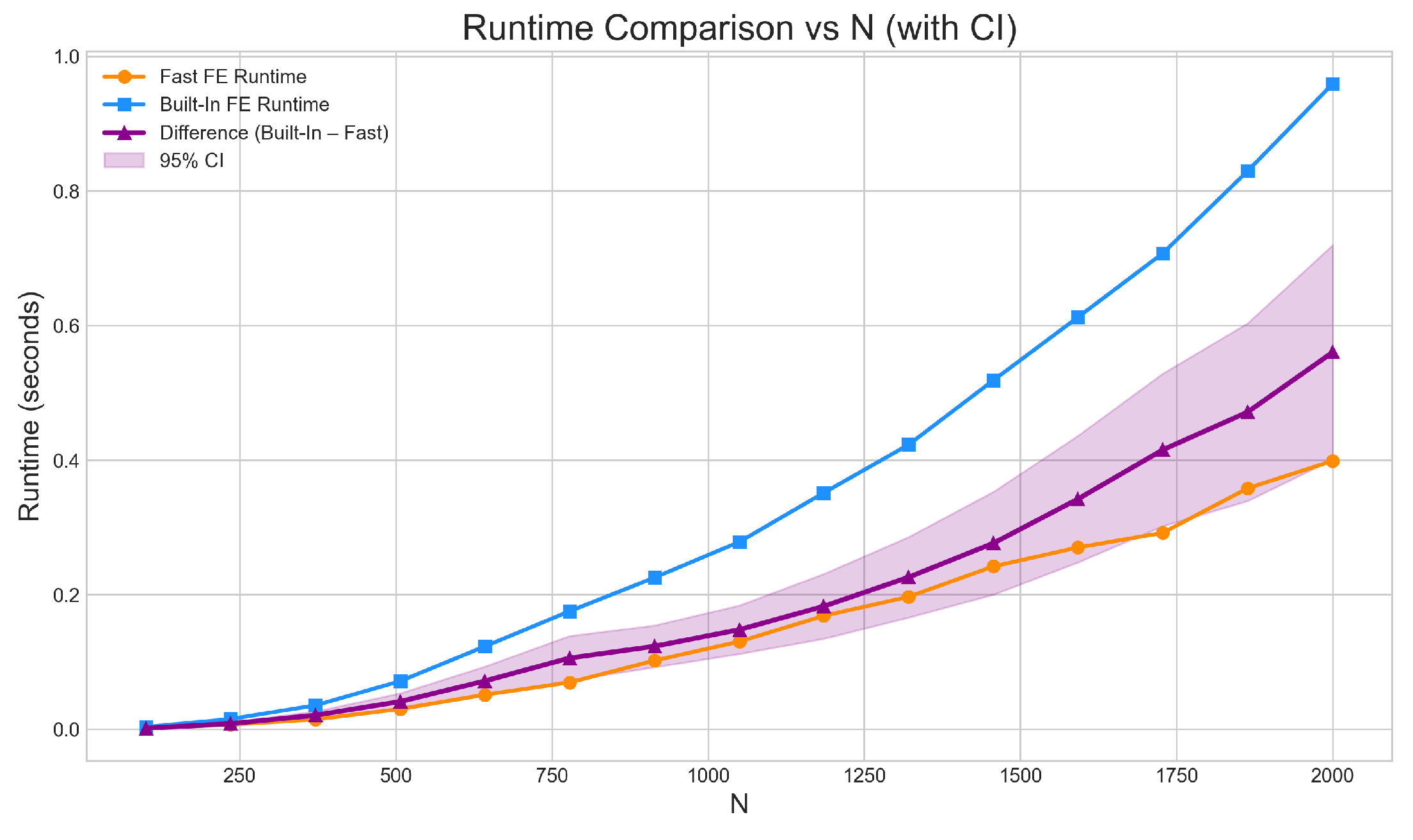
9.2. Computation Time as a Function of the Number of Periods

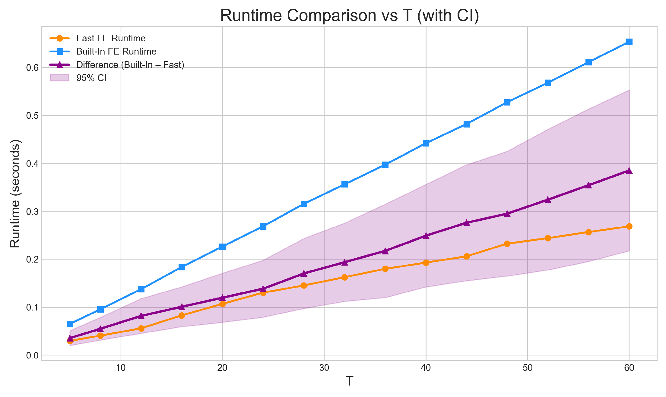
Figure 2. Computation time for fe_fast and the demeaned estimator as the number of periods T increases. Both estimators require more computation as T grows, with a stronger rise in run time for the demeaned approach. fe_fast maintains a lower run time throughout the grid.

Figure 2. Computation time for fe_fast and the demeaned estimator as the number of periods T increases. Both estimators require more computation as T grows, with a stronger rise in run time for the demeaned approach. fe_fast maintains a lower run time throughout the grid.

9.3. Computation Time Across $(\mathrm{N},\mathrm{T})$ Combinations

Figure 3. Average run time of fe_fast across combinations of sample size N and number of periods T. Computation increases smoothly with panel size due to grouped matrix updates.

Figure 3. Average run time of fe_fast across combinations of sample size N and number of periods T. Computation increases smoothly with panel size due to grouped matrix updates.

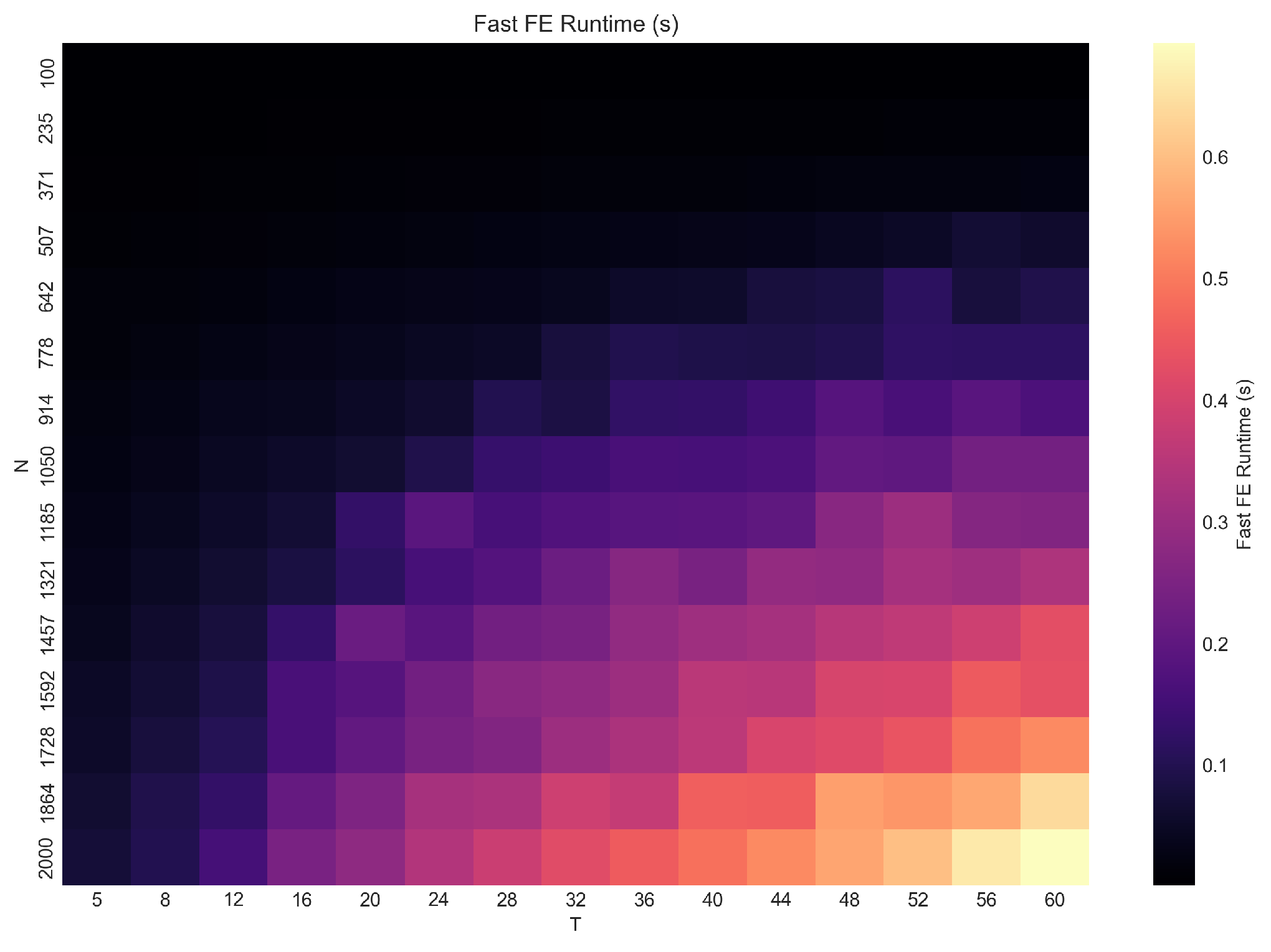
Figure 4. Average run time of the demeaned estimator across $(\mathrm{N},\mathrm{T})$. The required per-unit transformations lead to larger increases in run time relative to fe_fast, particularly when both N and T are large.

Figure 4. Average run time of the demeaned estimator across $(\mathrm{N},\mathrm{T})$. The required per-unit transformations lead to larger increases in run time relative to fe_fast, particularly when both N and T are large.

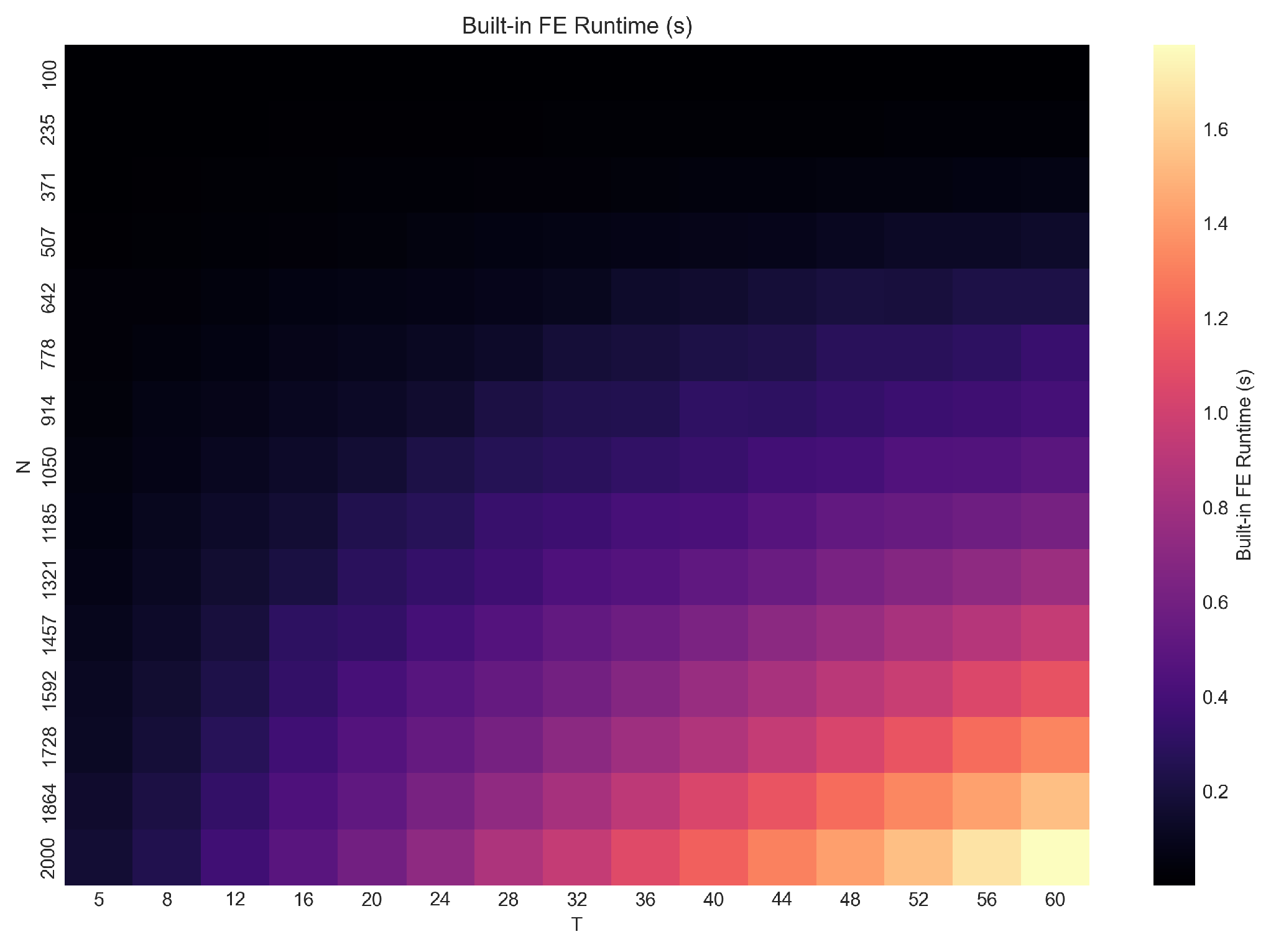
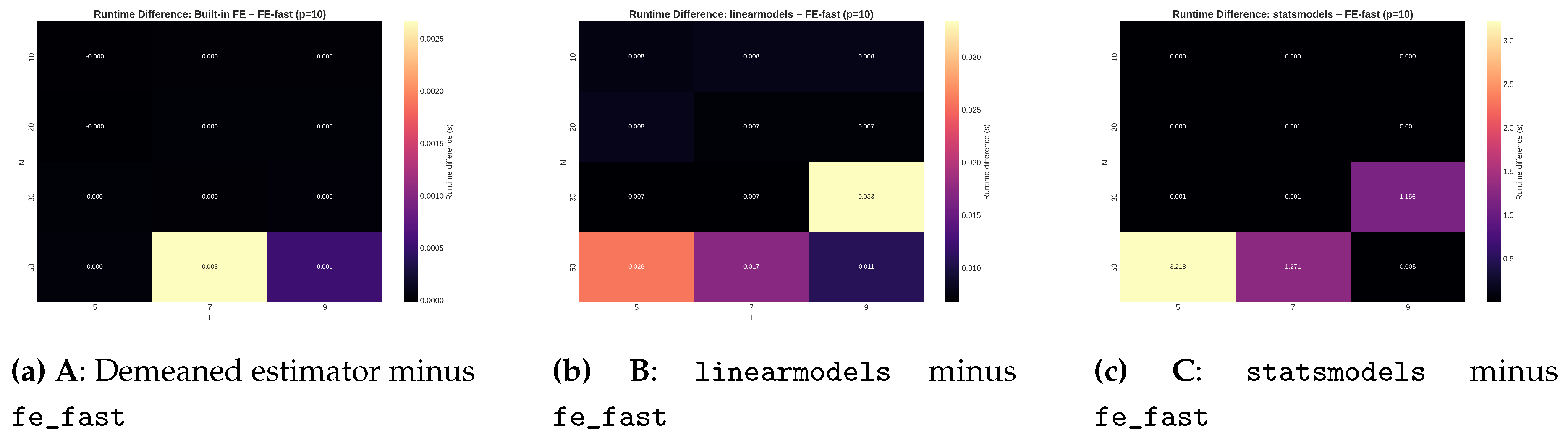
Figure 5. Differences in run time relative to fe_fast for $\mathrm{p}=10$. Each panel reports the average difference in computation time across $(\mathrm{N},\mathrm{T})$. Positive values indicate slower performance for the comparison estimator. The demeaned estimator (A) is slower throughout the grid. The linearmodels and statsmodels approaches (B, C) show larger delays due to block operations and dummy-variable expansions.

Figure 5. Differences in run time relative to fe_fast for $\mathrm{p}=10$. Each panel reports the average difference in computation time across $(\mathrm{N},\mathrm{T})$. Positive values indicate slower performance for the comparison estimator. The demeaned estimator (A) is slower throughout the grid. The linearmodels and statsmodels approaches (B, C) show larger delays due to block operations and dummy-variable expansions.

9.4. Memory Use Across $(\mathrm{N},\mathrm{T})$ Combinations

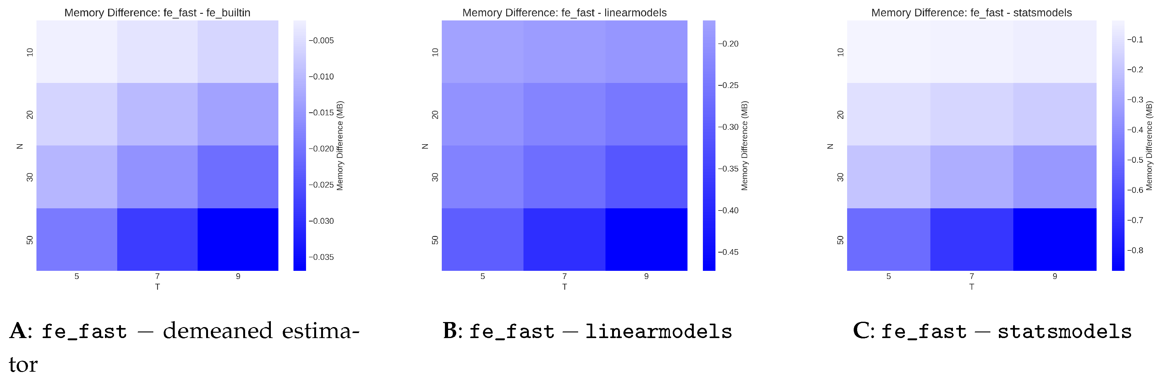
Figure 6. Memory use of fe_fast relative to three alternative estimators for $\mathrm{p}=10$. Each panel reports the difference in memory consumption across $(\mathrm{N},\mathrm{T})$. Negative values indicate lower memory use for fe_fast. The grouped estimator avoids repeated unit-level transformations and dummy construction, leading to lower use of temporary objects across nearly all settings.

Figure 6. Memory use of fe_fast relative to three alternative estimators for $\mathrm{p}=10$. Each panel reports the difference in memory consumption across $(\mathrm{N},\mathrm{T})$. Negative values indicate lower memory use for fe_fast. The grouped estimator avoids repeated unit-level transformations and dummy construction, leading to lower use of temporary objects across nearly all settings.

9.5. Coefficient Differences

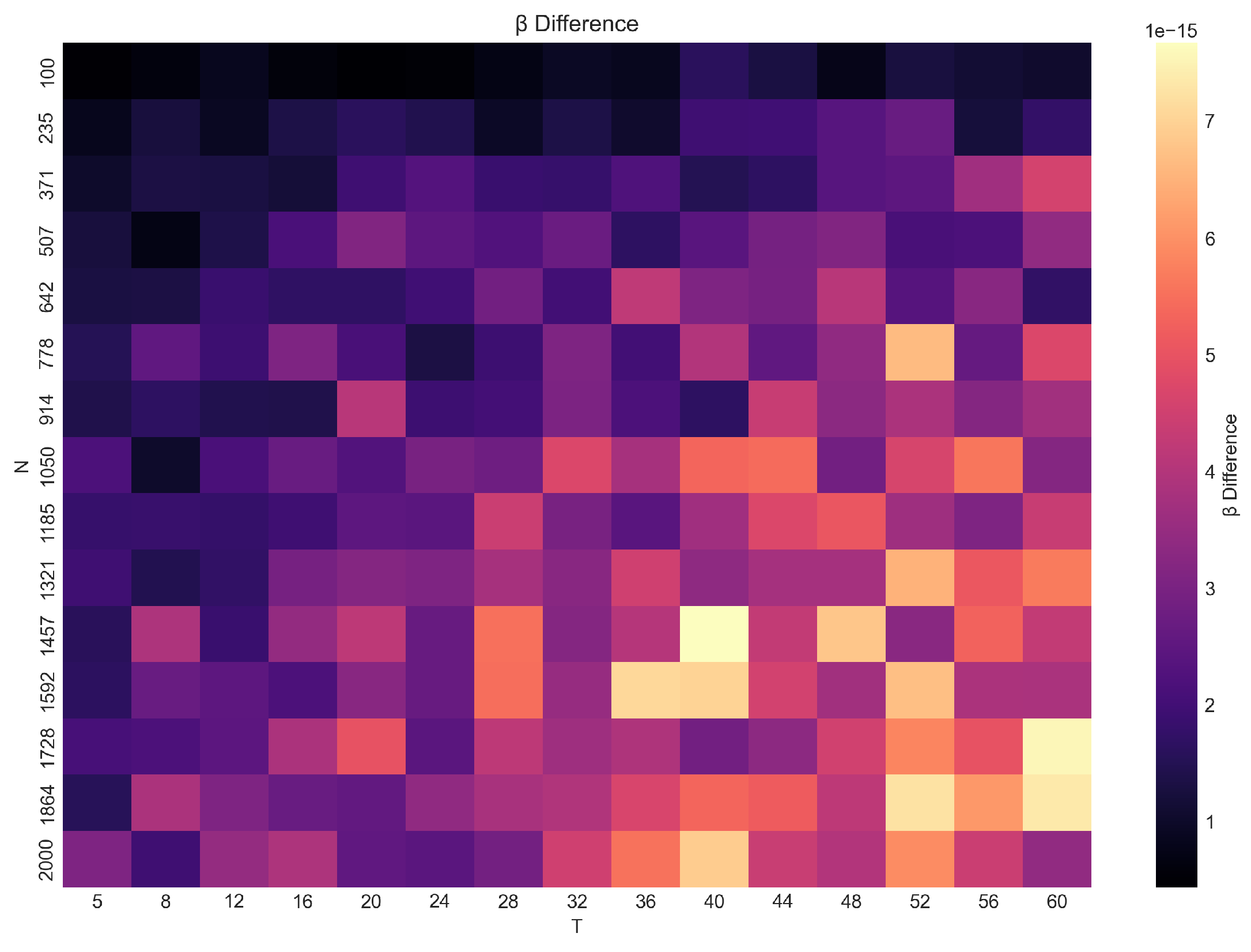
Figure 7. Absolute difference in slope estimates produced by fe_fast and the demeaned estimator across $(\mathrm{N},\mathrm{T})$. Differences remain close to numerical tolerance ($\le {10}^{14}$) across the grid, indicating close agreement between the two approaches.

Figure 7. Absolute difference in slope estimates produced by fe_fast and the demeaned estimator across $(\mathrm{N},\mathrm{T})$. Differences remain close to numerical tolerance ($\le {10}^{14}$) across the grid, indicating close agreement between the two approaches.

10. Computational Complexity

This section collects FLOP counts, byte-traffic expressions, and communication lower bounds for both the within and grouped estimators.

10.1. Floating-Point Operations

For each unit i:

$${\mathrm{G}}_{\mathrm{i}}=\sum _{\mathrm{t}=1}^{{\mathrm{T}}_{\mathrm{i}}}{\mathrm{x}}_{\mathrm{i}\mathrm{t}}{\mathrm{x}}_{\mathrm{i}\mathrm{t}}^{\prime }\cos \mathrm{ts}\mathcal{O}\left({\mathrm{T}}_{\mathrm{i}}{\mathrm{p}}^2\right),$$

$${\mathrm{g}}_{\mathrm{i}}=\sum _{\mathrm{t}=1}^{{\mathrm{T}}_{\mathrm{i}}}{\mathrm{x}}_{\mathrm{i}\mathrm{t}}{\mathrm{y}}_{\mathrm{i}\mathrm{t}}\cos \mathrm{ts}\mathcal{O}\left({\mathrm{T}}_{\mathrm{i}}\mathrm{p}\right).$$

Summed across units, the grouped estimator costs

$$\mathcal{O}\left(\mathrm{n}{\mathrm{p}}^2\right).$$

The within transformation forms ${\mathrm{x}}_{\mathrm{i}\mathrm{t}}^{*}$ explicitly:

$${\mathrm{x}}_{\mathrm{i}\mathrm{t}}^{*}={\mathrm{x}}_{\mathrm{i}\mathrm{t}}-{\overline{\mathrm{x}}}_{\mathrm{i}}\Rightarrow \mathcal{O}\left(\mathrm{n}\mathrm{p}\right)\mathrm{subtractions}.$$

The Gram matrix computed from demeaned arrays again costs $\mathcal{O}\left(\mathrm{n}{\mathrm{p}}^2\right)$. The FLOP gap between methods is therefore $\mathcal{O}\left(\mathrm{n}\mathrm{p}\right)$, which becomes negligible when p is small but matters once byte movement dominates arithmetic.

10.2. Byte-Traffic Characterization

Let B denote bytes per floating point value. For the within estimator, reading and writing the transformed arrays requires

$${\mathrm{Bytes}}_{\mathrm{within}}\approx 2\mathrm{n}\mathrm{p}\mathrm{B}.$$

The grouped estimator avoids all writes and performs only reads:

$${\mathrm{Bytes}}_{\mathrm{fast}}\approx \mathrm{n}\mathrm{p}\mathrm{B}.$$

The difference is a full pass of size $\mathrm{n}\mathrm{p}\mathrm{B}$, which aligns with the measured memory gap in the simulations.

10.3. Communication Lower Bound

The Hong–Kung red–blue pebble model implies that computing $\sum {\mathrm{x}}_{\mathrm{i}\mathrm{t}}^{*}{\mathrm{x}}_{\mathrm{i}\mathrm{t}}^{*\prime }$ from explicit transformed arrays requires

$$\mathrm{\Omega }\left(\mathrm{n}\mathrm{p}\right)$$

data movement. The grouped estimator bypasses this requirement by not materializing the centered arrays, reaching the lower bound for a single pass algorithm.

10.4. Roofline Interpretation

Performance is shaped by the ratio of FLOPs to bytes moved. The within estimator has arithmetic intensity roughly

$${\mathrm{I}}_{\mathrm{within}}\approx {\displaystyle \frac{\mathrm{p}}{2}},$$

whereas the grouped estimator reaches

$${\mathrm{I}}_{\mathrm{fast}}\approx \mathrm{p}.$$

Higher intensity shifts the algorithm toward the compute-bound region of the roofline.

11. Conclusion

Grouped Gram summaries provide a route to fixed effects estimation that yields lower memory traffic than the classical method based on transformed arrays. Both reach the same estimator. The difference lies in how intermediate values are assembled. As panels grow, memory traffic dominates floating point operations. A method that minimizes movement can produce substantial gains.

Appendix G.1. Proof of Theorem 1 (Fixed T, N→∞)

Units form independent clusters.

$${\mathrm{X}}_{\mathrm{i}}\stackrel{\mathrm{def}}{=}\left[\begin{array}{c}{\mathrm{x}}_{\mathrm{i}1}^{\prime }\\ ⋮\\ {\mathrm{x}}_{\mathrm{i}{\mathrm{T}}_{\mathrm{i}}}^{\prime }\end{array}\right],{\mathrm{y}}_{\mathrm{i}}\stackrel{\mathrm{def}}{=}\left[\begin{array}{c}{\mathrm{y}}_{\mathrm{i}1}\\ ⋮\\ {\mathrm{y}}_{\mathrm{i}{\mathrm{T}}_{\mathrm{i}}}\end{array}\right],{\mathrm{M}}_{\mathrm{i}}\stackrel{\mathrm{def}}{=}{\mathrm{I}}_{{\mathrm{T}}_{\mathrm{i}}}-{\displaystyle \frac{1}{{\mathrm{T}}_{\mathrm{i}}}}11^{\prime }.$$

The within-transformed variables satisfy

$${\mathrm{X}}_{\mathrm{i}}^{*}\stackrel{\mathrm{def}}{=}{\mathrm{M}}_{\mathrm{i}}{\mathrm{X}}_{\mathrm{i}},{\mathrm{y}}_{\mathrm{i}}^{*}\stackrel{\mathrm{def}}{=}{\mathrm{M}}_{\mathrm{i}}{\mathrm{y}}_{\mathrm{i}}.$$

Step 1: Gram Identity

Start from

$${\mathrm{X}}_{\mathrm{i}}^{*\prime }{\mathrm{X}}_{\mathrm{i}}^{*}={\mathrm{X}}_{\mathrm{i}}^{\prime }{\mathrm{M}}_{\mathrm{i}}{\mathrm{X}}_{\mathrm{i}}={\mathrm{X}}_{\mathrm{i}}^{\prime }{\mathrm{X}}_{\mathrm{i}}-{\displaystyle \frac{1}{{\mathrm{T}}_{\mathrm{i}}}}{\mathrm{X}}_{\mathrm{i}}^{\prime }11^{\prime }{\mathrm{X}}_{\mathrm{i}}.$$

Use

$${\mathrm{X}}_{\mathrm{i}}^{\prime }{\mathrm{X}}_{\mathrm{i}}=\sum _{\mathrm{t}=1}^{{\mathrm{T}}_{\mathrm{i}}}{\mathrm{x}}_{\mathrm{i}\mathrm{t}}{\mathrm{x}}_{\mathrm{i}\mathrm{t}}^{\prime },{\mathrm{X}}_{\mathrm{i}}^{\prime }1=\sum _{\mathrm{t}=1}^{{\mathrm{T}}_{\mathrm{i}}}{\mathrm{x}}_{\mathrm{i}\mathrm{t}}={\mathrm{s}}_{\mathrm{x},\mathrm{i}}.$$

Thus

$${\mathrm{X}}_{\mathrm{i}}^{*\prime }{\mathrm{X}}_{\mathrm{i}}^{*}={\mathrm{G}}_{\mathrm{i}}-{\displaystyle \frac{{\mathrm{s}}_{\mathrm{x},\mathrm{i}}{\mathrm{s}}_{\mathrm{x},\mathrm{i}}^{\prime }}{{\mathrm{T}}_{\mathrm{i}}}}.$$

Similarly,

$${\mathrm{X}}_{\mathrm{i}}^{*\prime }{\mathrm{y}}_{\mathrm{i}}^{*}={\mathrm{g}}_{\mathrm{i}}-{\displaystyle \frac{{\mathrm{s}}_{\mathrm{x},\mathrm{i}}{\mathrm{s}}_{\mathrm{y},\mathrm{i}}}{{\mathrm{T}}_{\mathrm{i}}}}.$$

The grouped and demeaned estimators solve the same equation.

Step 2: Score Expansion

Let the within residual be

$${\mathrm{u}}_{\mathrm{i}}={\mathrm{y}}_{\mathrm{i}}^{*}-{\mathrm{X}}_{\mathrm{i}}^{*}\mathrm{\beta }.$$

Define the cluster score

$${\mathrm{S}}_{\mathrm{i}}={\mathrm{X}}_{\mathrm{i}}^{*\prime }{\mathrm{u}}_{\mathrm{i}}.$$

The estimator solves

$$0=\sum _{\mathrm{i}=1}^{\mathrm{N}}{\mathrm{X}}_{\mathrm{i}}^{*\prime }({\mathrm{y}}_{\mathrm{i}}^{*}-{\mathrm{X}}_{\mathrm{i}}^{*}\widehat{\mathrm{\beta }}),$$

which rearranges to

$$\left(\sum _{\mathrm{i}=1}^{\mathrm{N}}{\mathrm{X}}_{\mathrm{i}}^{*\prime }{\mathrm{X}}_{\mathrm{i}}^{*}\right)(\widehat{\mathrm{\beta }}-\mathrm{\beta })=\sum _{\mathrm{i}=1}^{\mathrm{N}}{\mathrm{S}}_{\mathrm{i}}.$$

Multiply both sides by $\sqrt{\mathrm{N}}$:

$$\sqrt{\mathrm{N}}(\widehat{\mathrm{\beta }}-\mathrm{\beta })={\left({\displaystyle \frac{1}{\mathrm{N}}}\sum _{\mathrm{i}=1}^{\mathrm{N}}{\mathrm{X}}_{\mathrm{i}}^{*\prime }{\mathrm{X}}_{\mathrm{i}}^{*}\right)}^{-1}\left({\displaystyle \frac{1}{\sqrt{\mathrm{N}}}}\sum _{\mathrm{i}=1}^{\mathrm{N}}{\mathrm{S}}_{\mathrm{i}}\right).$$

Step 3: Law of Large Numbers (LLN) for the Hessian

With T fixed,

$${\displaystyle \frac{1}{\mathrm{N}}}\sum _{\mathrm{i}=1}^{\mathrm{N}}{\mathrm{X}}_{\mathrm{i}}^{*\prime }{\mathrm{X}}_{\mathrm{i}}^{*}\stackrel{\mathrm{p}}{\to }\mathrm{Q}=\mathbb{E}\left[{\mathrm{X}}_{\mathrm{i}}^{*\prime }{\mathrm{X}}_{\mathrm{i}}^{*}\right].$$

Step 4: Central Limit Theorem (CLT) for the Score

Cluster independence implies

$${\displaystyle \frac{1}{\sqrt{\mathrm{N}}}}\sum _{\mathrm{i}=1}^{\mathrm{N}}{\mathrm{S}}_{\mathrm{i}}\stackrel{\mathrm{d}}{\to }\mathcal{N}(0,\mathrm{\Omega }),\mathrm{\Omega }=\mathbb{E}\left[{\mathrm{S}}_{\mathrm{i}}{\mathrm{S}}_{\mathrm{i}}^{\prime }\right].$$

Step 5: Combine Limits

Slutsky yields

$$\sqrt{\mathrm{N}}(\widehat{\mathrm{\beta }}-\mathrm{\beta })\stackrel{\mathrm{d}}{\to }{\mathrm{Q}}^{-1}\mathrm{\Omega }{\mathrm{Q}}^{-1}.$$

This completes the fixed-T theorem.

Appendix G.2. Proof of Theorem 2 (Large N,T, n=NT→∞)

Balanced panel assumed for exposition.

Start from the FOC,

$$0=\sum _{\mathrm{i}=1}^{\mathrm{N}}\sum _{\mathrm{t}=1}^{\mathrm{T}}{\mathrm{x}}_{\mathrm{i}\mathrm{t}}^{*}({\mathrm{y}}_{\mathrm{i}\mathrm{t}}^{*}-{\mathrm{x}}_{\mathrm{i}\mathrm{t}}^{*\prime }\widehat{\mathrm{\beta }}).$$

Substitute

$${\mathrm{y}}_{\mathrm{i}\mathrm{t}}^{*}={\mathrm{x}}_{\mathrm{i}\mathrm{t}}^{*\prime }\mathrm{\beta }+{\mathrm{u}}_{\mathrm{i}\mathrm{t}},$$

to obtain

$$\left(\sum _{\mathrm{i},\mathrm{t}}{\mathrm{x}}_{\mathrm{i}\mathrm{t}}^{*}{\mathrm{x}}_{\mathrm{i}\mathrm{t}}^{*\prime }\right)(\widehat{\mathrm{\beta }}-\mathrm{\beta })=\sum _{\mathrm{i},\mathrm{t}}{\mathrm{x}}_{\mathrm{i}\mathrm{t}}^{*}{\mathrm{u}}_{\mathrm{i}\mathrm{t}}.$$

Divide by $\sqrt{\mathrm{n}}=\sqrt{\mathrm{N}\mathrm{T}}$:

$$\sqrt{\mathrm{n}}(\widehat{\mathrm{\beta }}-\mathrm{\beta })={\left({\displaystyle \frac{1}{\mathrm{n}}}\sum _{\mathrm{i},\mathrm{t}}{\mathrm{x}}_{\mathrm{i}\mathrm{t}}^{*}{\mathrm{x}}_{\mathrm{i}\mathrm{t}}^{*\prime }\right)}^{-1}\left({\displaystyle \frac{1}{\sqrt{\mathrm{n}}}}\sum _{\mathrm{i},\mathrm{t}}{\mathrm{x}}_{\mathrm{i}\mathrm{t}}^{*}{\mathrm{u}}_{\mathrm{i}\mathrm{t}}\right).$$

Step 1: Convergence of the Hessian

Under stationarity and mixing conditions,

$${\displaystyle \frac{1}{\mathrm{n}}}\sum _{\mathrm{i},\mathrm{t}}{\mathrm{x}}_{\mathrm{i}\mathrm{t}}^{*}{\mathrm{x}}_{\mathrm{i}\mathrm{t}}^{*\prime }\stackrel{\mathrm{p}}{\to }\mathrm{Q}.$$

Step 2: Central Limit Theorem (CLT) for Weak Dependence

The term

$${\displaystyle \frac{1}{\sqrt{\mathrm{n}}}}\sum _{\mathrm{i},\mathrm{t}}{\mathrm{x}}_{\mathrm{i}\mathrm{t}}^{*}{\mathrm{u}}_{\mathrm{i}\mathrm{t}}$$

satisfies a mixingale or strong-mixing CLT:

$${\displaystyle \frac{1}{\sqrt{\mathrm{n}}}}\sum _{\mathrm{i},\mathrm{t}}{\mathrm{x}}_{\mathrm{i}\mathrm{t}}^{*}{\mathrm{u}}_{\mathrm{i}\mathrm{t}}\stackrel{\mathrm{d}}{\to }\mathcal{N}(0,\mathrm{\Omega }).$$

Step 3: Combine Limits

Thus,

$$\sqrt{\mathrm{n}}(\widehat{\mathrm{\beta }}-\mathrm{\beta })\stackrel{\mathrm{d}}{\to }{\mathrm{Q}}^{-1}\mathrm{\Omega }{\mathrm{Q}}^{-1}.$$

The result matches the demeaned estimator; both share the same algebraic structure.

Appendix G.3. Symbolic Verification of the Gram Identity

The identity

$$\sum _{\mathrm{t}=1}^{{\mathrm{T}}_{\mathrm{i}}}({\mathrm{x}}_{\mathrm{i}\mathrm{t}}-{\overline{\mathrm{x}}}_{\mathrm{i}}){({\mathrm{x}}_{\mathrm{i}\mathrm{t}}-{\overline{\mathrm{x}}}_{\mathrm{i}})}^{\prime }\equiv {\mathrm{G}}_{\mathrm{i}}-{\displaystyle \frac{{\mathrm{s}}_{\mathrm{x},\mathrm{i}}{\mathrm{s}}_{\mathrm{x},\mathrm{i}}^{\prime }}{{\mathrm{T}}_{\mathrm{i}}}}$$

was checked using a symbolic solver.

References

- Arellano, M. Panel Data Econometrics; Oxford University Press, 2003. [Google Scholar]
- Cameron, A. C.; Gelbach, J. B.; Miller, D. L. Bootstrap-Based Improvements for Inference with Clustered Errors. Review of Economics and Statistics 2008, 90(3), 414–427. [Google Scholar] [CrossRef]
- Chan, T. F.; Golub, G. H. Updating Formulae and a Pairwise Algorithm for Computing Sample Variances. Journal of the Royal Statistical Society: Series C 1983, 32(3), 266–274. [Google Scholar]
- Davison, A. C.; Hinkley, D. V. Bootstrap Methods and Their Application; Cambridge University Press, 1997. [Google Scholar]
- Demmel, J.; Grigori, L.; Hoemmen, M.; Langou, J. Communication-Avoiding Linear Algebra. SIAM Review 2007, 53(1), 1–20. [Google Scholar]
- Gentle, J. E. Matrix Algebra: Theory, Computations, and Applications; Springer, 2007. [Google Scholar]
- Golub, G. H.; Van Loan, C. F. Matrix Computations, 4th ed.; Johns Hopkins University Press, 2013. [Google Scholar]
- Graham, S. L.; Snir, M.; Patterson, D. Getting Up to Speed: The Future of Supercomputing; National Research Council Report, 2002. [Google Scholar]
- Hausman, J. A. Specification Tests in Econometrics. Econometrica 1978, 46(6), 1251–1271. [Google Scholar] [CrossRef]
- Holtz-Eakin, D.; Newey, W.; Rosen, H. Estimating Vector Autoregressions with Panel Data. Econometrica 1988, 56(6), 1371–1395. [Google Scholar] [CrossRef]
- Hong, J. W.; Kung, H. T. I/O Complexity: The Red-Blue Pebble Game. Proceedings of STOC, 1981; pp. 326–333. [Google Scholar]
- Hsiao, C. Analysis of Panel Data; Cambridge University Press, 2014. [Google Scholar]
- Lindsay, B. Composite Likelihood Methods. In Proceedings of the Section on Statistical Theory, ASA, 1988. [Google Scholar]
- McCalpin, J. STREAM: Sustainable Memory Bandwidth in High Performance Computers. Technical Report, 1995. [Google Scholar]
- McCullagh, P.; Nelder, J. Generalized Linear Models; Chapman and Hall, 1989. [Google Scholar]
- Mundlak, Y. On the Pooling of Time Series and Cross Section Data. Econometrica 1978, 46(1), 69–85. [Google Scholar] [CrossRef]
- Nickell, S. Biases in Dynamic Models with Fixed Effects. Econometrica 1981, 49(6), 1417–1426. [Google Scholar] [CrossRef]
- Williams, S.; Waterman, A.; Patterson, D. Roofline: An Insightful Visual Performance Model for Floating-Point Programs and Multicore Architectures. Communications of the ACM 2009, 52(4), 65–76. [Google Scholar] [CrossRef]
- Wooldridge, J. M. Econometric Analysis of Cross Section and Panel Data; MIT Press, 2010. [Google Scholar]
Disclaimer/Publisher’s Note: The statements, opinions and data contained in all publications are solely those of the individual author(s) and contributor(s) and not of MDPI and/or the editor(s). MDPI and/or the editor(s) disclaim responsibility for any injury to people or property resulting from any ideas, methods, instructions or products referred to in the content. |
© 2025 by the authors. Licensee MDPI, Basel, Switzerland. This article is an open access article distributed under the terms and conditions of the Creative Commons Attribution (CC BY) license (http://creativecommons.org/licenses/by/4.0/).
Copyright: This open access article is published under a Creative Commons CC BY 4.0 license, which permit the free download, distribution, and reuse, provided that the author and preprint are cited in any reuse.