Optimizing Retail Decision-Making Through Big Data and Machine Learning Integration

1. Real-Time Data Processing in Retail

Overview

The term big data is used to describe vast sets of structured and unstructured data that are generated from different sources, including digital libraries, social networks, mobile apps, internet clickstream logs, emails, documents, and customer databases, among others (Guru & Bajnaid, 2023). The analysis of these sets of data is referred to as big data analytics and it involves the systematic collection, processing, and interpretation of the data to extract valuable insights that can be used to make informed decisions.

In retail, big data analytics has become paramount over the past few decades due to its ability to provide valuable and actionable knowledge to businesses. With large amounts of data being generated daily from social networks, customer transactions, and online interactions, big data analytics has emerged as one of the key drivers of success for businesses in the retail sector (Hammond-Errey, 2023). By helping businesses get key insights into customer behavior and their purchasing patterns, how each product is performing, the current market trends, and the efficiency of supply chains, it helps them make informed decisions that can improve their profitability. For instance, it allows them to know which operations should be optimized, how to tailor their marketing campaigns, and how their pricing should be adjusted to stay competitive and improve their sales.

As highlighted by Giri et al. (2019), analyzing big data requires specialized tools. This is because big data is essentially characterized by three key aspects:

• Volume – it comprises particularly large sets of data that traditional storage and processing systems cannot handle efficiently.
• Velocity - it is generated at very high speeds, and is required to be collected and processed in real-time. For instance, streaming data from social media platforms like YouTube or Instagram.
• Variety – it is collected in different forms, including structured, such as databases; semi-structured such as logs and JSON; and unstructured data such as videos, images, and text (Guru & Bajnaid, 2023).

As such, various technologies and tools are employed to collect, process, and transform this complex and heterogeneous data into something useful that can be used by the business to make informed decisions and optimize their operations accordingly. For instance, emerging technologies like IoT (Internet of Things), AI (artificial intelligence), and machine learning are being implemented for big data analytics (Niu & He, 2019).

Big Data Technologies

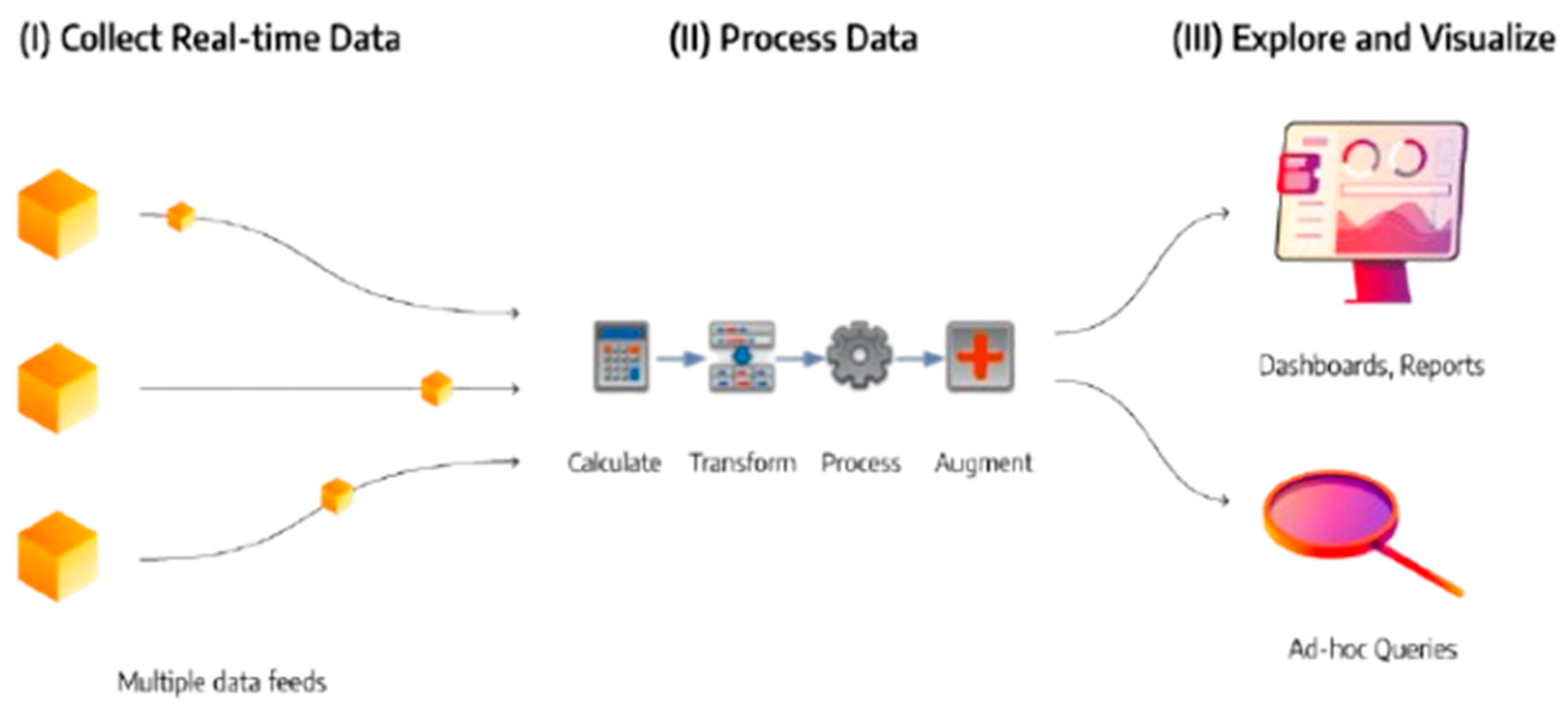
These include the various tools and techniques that are utilized to mine, clean, integrate, and visualize big data in real time to make it easy for businesses to obtain valuable insights from large, varying, and complex sets of data (Ravi, 2024). This allows them to personalize their marketing strategies and improve customer interactions. For instance, technologies like Apache Kafka and Google BigQuery facilitate the real-time processing of continuous vast data from social networks, e-commerce sites, and customer interactions. Major companies like LinkedIn, Netflix, Uber, Airbnb, and Spotify use Kafka and BigQuery to process and analyze vast, real-time datasets (Sharma et al., 2021). They allow them to create personalized recommendations to improve user experiences, get valuable insights into customer preferences, and make data-driven decisions to improve their productivity. This process follows a specific structure that involves data being collected from multiple sources, immediate computations, such as statistical measures and aggregations, being performed to transform the collected raw data into meaningful formats, and visual representations of the processed data being produced in form of data trends and patterns to help the retailer make informed decisions about their business operations.

Figure 1. A typical process in real-time big data analytics.

Figure 1. A typical process in real-time big data analytics.

These recommendations can be in the form of:

• Dynamic recommendations, whereby users are given suggestions in real-time according to how they interact with the platform and/or their preferences (Solanki et al., 2022). Take, for instance, an individual visiting an e-commerce platform, the program analyzes their previous purchases, search history, and related information to recommend products as they are browsing.
• Targeted promotions, in which the customer is sent tailored discounts and/or offers through the platform, SMS, or email while they are actively using the platform.
• Geo-targeted ads, whereby the customer receives specific alerts or advertisements depending on their current location (Thakur, 2023).

According to Guru & Bajnaid (2023), retailers are able to make such quick and data-driven recommendations due to real-time data processing enabled by data analytics and machine learning algorithms. For instance, retail giant Amazon provides real-time product recommendations to customers using machine learning-powered big data technologies like AWS Machine Learning Services and Amazon Personalize which analyze customers’ purchase history, behavior patterns, and browsing activities in real-time to provide suggestions in the “Customers Also Bought” section.

In conclusion, Big data analytics makes it easy for businesses in the retail industry to uncover correlations, patterns, and trends in vast volumes of raw data. Extracting and analyzing this data is a complex process that leverages big data technologies that employ data analytics and machine learning algorithms (Sharma et al., 2021). This process enables businesses to take advantage of the rapidly increasing data generated from varied sources, including point-of-sale systems, online purchases, social media interactions, and loyalty programs, among others to obtain actionable intelligence via advanced analytic systems. This intelligence is significant for providing deeper insight into customer behavior, predicting customer preferences, and consequently, future trends, all of which play a major role in boosting the customer experience.

2. Data Analytics and Machine Learning Algorithms

Overview

The data collected for big data analytics is normally vast and varied, comprising structured data like databases; semi-structured such as logs and JSON; and unstructured data such as videos, images, and text (Guru & Bajnaid, 2023). This makes it very hard to manage the data or get useful insight using traditional methods like paper-based analysis, visual inspection, simple calculations, checklists, tally sheets, and comparative analysis. These methods are labor-intensive, prone to errors, and thus, not fitting for analyzing large or complex datasets. For instance, according to a recent report by Invisibly, the giant retailer Amazon collects and processes about 1 exabyte of purchase history data from its customer base for big data analytics. Using the aforementioned traditional methods to collect or analyze this data would be very challenging. As such, AI-powered methods are used to extract, transform, and process this data to make it easy to study patterns related to current trends, customer behavior, and their interactions (Ravi, 2024). This helps the company in a number of ways including, inventory management optimization, personalization of marketing strategies, improvement of pricing strategies, operational efficiency enhancement, fraud detection and security enhancement, and improvement of customer support.

Machine Learning Algorithms for Customer Experience Optimization

These AI-powered methods specifically employ machine learning algorithms to facilitate various processes, including automation of repetitive tasks, sentiment analysis, and prediction of customer needs (Solanki et al., 2022). For instance, statistical algorithms, such as linear regression, are used by retail companies like Walmart to analyze historical data and other related information to predict customer behavior and sales and adjust their operations accordingly. Machine learning algorithms, such as collaborative filtering, clustering algorithms, and NLP (natural language processing), are largely used by Amazon to analyze sentiment and textual data such as customer reviews to better understand their preferences and adjust accordingly (Ravi, 2024). This helps the company enhance product recommendations, and improve their services, for a better customer experience.

For instance, Apache Spark, which is one of the common big data analytics programs, being used by world’s leading retailers like Amazon, Walmart, Alibaba, Target, and eBay, among others, utilizes a machine learning-based library called MLlib (Luu, 2021). This library leverages key machine learning algorithms to facilitate the collection, processing, analysis, and visualization of big data. These include machine learning algorithms like:

• Linear regression – this helps to facilitate the prediction of numerical outcomes, for example in sales forecasting (Thakur, 2023).
• K-Means clustering – this helps facilitate customer segmentation in which similar customers are grouped according to their purchasing behaviors.
• Decision Trees – this helps in classification tasks like fraud detection.
• Collaborative Filtering – this is used in recommendation systems to suggest products and services to customers in real-time on e-commerce sites (Thakur, 2023).

Types of Data Analytics

Depending on the specific business or analysis objective, there are four key data analytic methods that can be applied to help retailers extract valuable insights from complex unstructured big data (Giri et al., 2019). Each of these methods includes a specific purpose to help retailers make informed decisions and improve customer experience. They include:

• Descriptive analytics – this focuses on the analysis of past related data such as customer behavior, preferences, and trends to provide insights into how customers interacted with the business in the past (Tolulope, 2022). For instance, Amazon analyzes customer purchase history and satisfaction survey data to determine the most popular products or the categories with the highest customer visitation.
• Diagnostic analytics – this involves the factor or reasons behind specific customer behavior being investigated to determine their root cause (Guru & Bajnaid, 2023). For instance, it can involve the company reviewing submitted customer complaints and returned products to determine why a specific product is not performing as expected or why someone would be dissatisfied with it. A good example of this in practice is with Target, which employs diagnostic analysis to investigate why sales are declining in specific stores by analyzing regional customer behavior, competitor activity, and local economic conditions to determine the reason why (Cote, 2021).
• Predictive analytics - in this, past data, such as past customer shopping patterns, is used to forecast customer preferences, behaviors, and market trends (Shi, 2022). This could help the company learn which products are likely to sell more in a specific season. Therefore, it could help the retailer tailor its marketing campaigns and inventory planning to improve customer experience and boost sales. For instance, Walmart employs machine learning algorithms to forecast demand for seasonal products such as holiday decorations or back-to-school supplies, to ensure that the inventory levels are optimum (Yi, 2023).
• Prescriptive analytics – this suggests the best action to take to enhance business operations and improve customer experience (Tolulope, 2022). For instance, the analytics tool can provide recommendations on how to personalize offers, adjust store layout, or improve product availability based on data from customer feedback and predictive models. The goal of this data analytics method is to meet the customer expectations to improve their experience. This has been applied successfully by Macy’s via dynamic pricing algorithms capable of adjusting prices in real time based on demand forecasts, competitor pricing, and stock levels, maximizing profitability while maintaining reasonable pricing (Chandramouli, 2023).

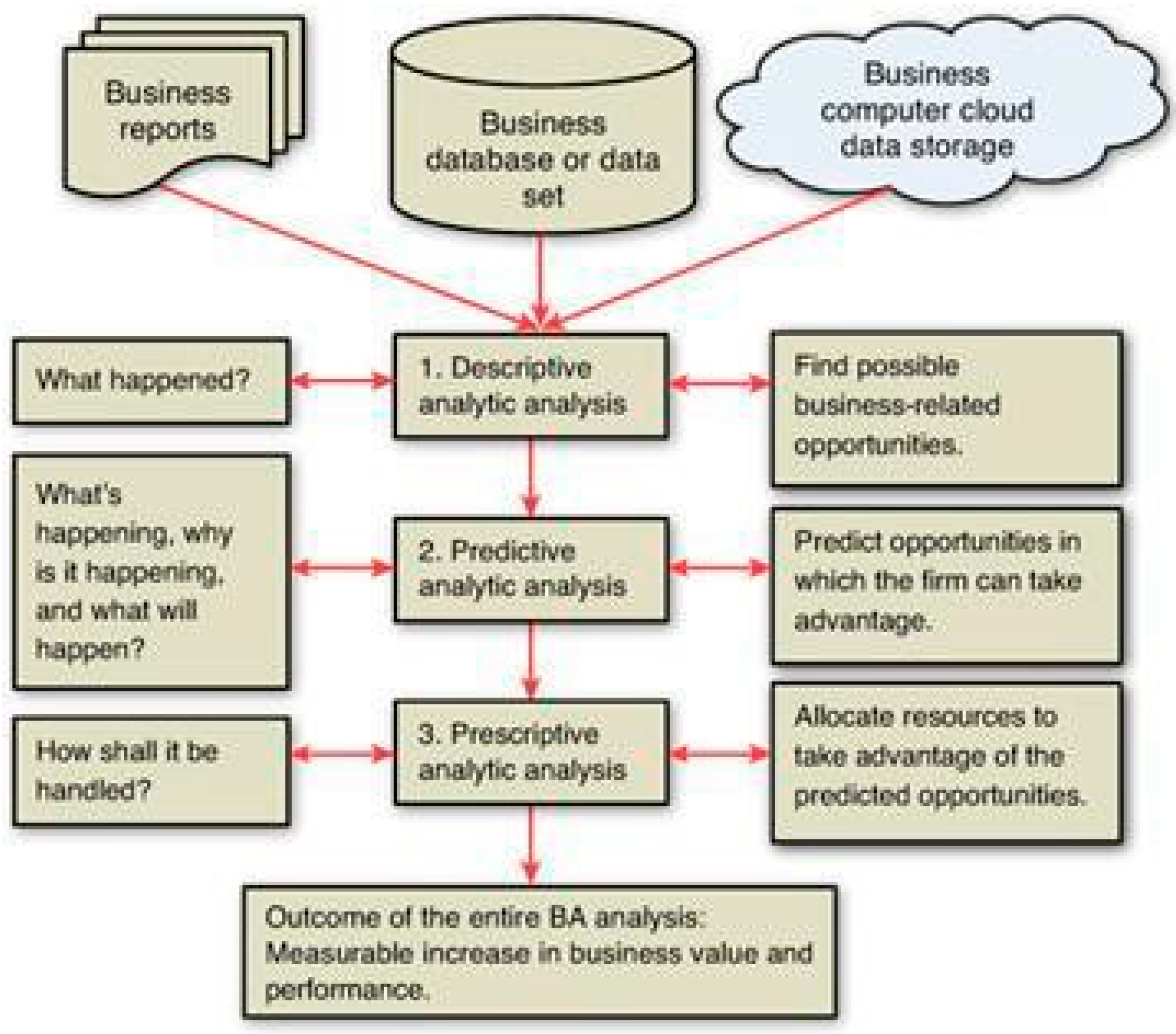
In reality, most retail companies leverage a combination of these analytics methods to provide key insights and improve decision-making at various stages of operation (Shi, 2022). For instance, as indicated in Figure 1 below, the company could begin with descriptive analytics to have a clearer picture of past performances of a specific product, followed by diagnostic analytics to ascertain the reasons behind those specific performances, then utilize predictive analytics to predict how the product might perform, and lastly use prescriptive analytics to determine the best actions to take to improve customer experience.

Figure 2. A typical business analytic process depicting a combination of the different analytic methods.

Figure 2. A typical business analytic process depicting a combination of the different analytic methods.

Machine learning algorithms serve a major role in big data analytics for retail. They simplify the processes of processing and analyzing vast amounts of customer, transaction, and inventory data in real-time to uncover trend patterns, optimize inventory, enhance marketing strategies, predict customer behavior, and provide personalized recommendations to improve customer experience. This is why more companies have started to integrate AI-based data analytics [37,38,39,40] and the trend is expected to grow. In fact, according to Gartner, the integration of AI technology will play key role in retail in the next few years, with integration in almost 80% of customer service and support services for improved customer experience and satisfaction (Gartner, 2024).

3. Key Considerations for Designing a Scalable Solution

In designing a scalable and efficient big data solution for retail, it is important to consider important aspects such as storage, processing speed and the integration of multiple data sources. Due to the high volume of data being generated by the retail industry, big data solutions and technology play an important role in improving the retail industry in terms of analysing customers’ behaviour, improving customer service and increasing sales [41,42,43].

In terms of storage, the retail industry generates many different types of data which includes inventory data, transactional data and more. Therefore, it is important to have a scalable and efficient storage system in place. To handle the amount of data being generated, a distributed storage system would be the best choice as the data will be distributed across different storage devices which allows for easy and efficient management and security. [1]

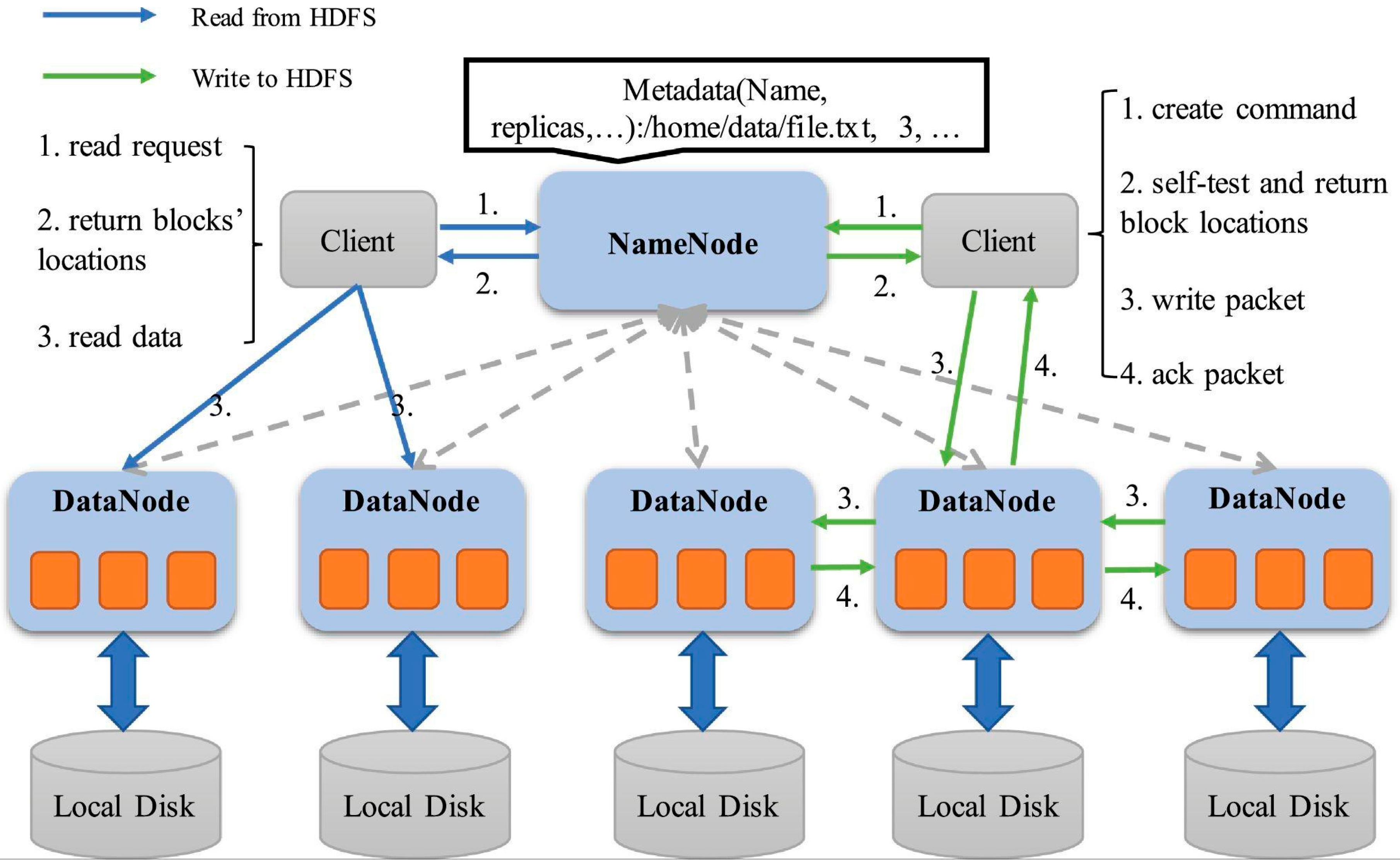
An example of a distributed storage system is the Hadoop Distributed File System (HDFS). The HDFS utilises a master-slave architecture where the entire HDFS framework is managed by NameNode (NN) and files are stored in the DataNodes (DNs). Hadoop will divide the data blocks and store them in different DNs. In case of a DN failure, each data block is replicated by default 3 times on several DNs with Hadoop’s replication system. [2] With the utilisation of MapReduce methodology, Hadoop is capable of performing parallel computing. Data will be divided into smaller chunks and be processed separately which improves the way data are stored and processed. [3]

Figure 3. Hadoop Distributed File System Architecture.

Figure 3. Hadoop Distributed File System Architecture.

In terms of processing speed, due to the high volume of data, it is pivotal to ensure that the data are being handled and processed efficiently to derive valuable analysis that will help improve the retail industry. The MapReduce methodology in Apache Hadoop enables the parallel processing of a large number of datasets which consequently improves the speed of data processing. Other than that, in-memory processing would significantly increase the data processing. An example would be Apache Spark. Spark utilises memory to store data which decreases the read/write cycle which is the slowing factor of processing speed in the Hadoop MapReduce framework. [3]

The retail industry operates across different platforms and systems, where a high volume of data is individually generated. These sources include the POS system, e-commerce platforms and supply chains. Therefore it is important to implement a system where the integration of multiple data sources is done efficiently. Apache Kafka is a tool that will allow effective data integration. Kafka allows the real-time streamlining of data and real-time data processing [44,45,46,47,48]. Other than that, Kafka utilises partitions for scale and multiple replicas which promotes durability and fault

tolerance. In the context of the retail industry, data from different sources can be assigned to a partition where they will be individually processed. The processing is mostly done in parallel as each partition is stored on a different broker. [4]

In conclusion, when designing a scalable and efficient big data solution for retail, it’s important to prioritise the storage, processing speed and integration with different sources due to the high amount of data being generated and collected. An effective solution would be a distributed computing system for storage and processing speed where data are distributed across different nodes or machines to be processed or analysed. This helps with the efficiency and scalability of data analytics.

4. Dataset Introduction

Table 1. Dataset.

Dataset Title	Online Sales Dataset
Dataset Link	https://www.kaggle.com/datasets/yusufdelikkaya/online-sales-dataset

Table 1. Dataset.

Dataset Title	Online Sales Dataset
Dataset Link	https://www.kaggle.com/datasets/yusufdelikkaya/online-sales-dataset

4.1. Dataset Size and Key Features Description

The dataset introduced a transactional history of customers, so analysis is made to better understand consumer behaviour, sales strategies optimization, and trends prediction.

The dataset has some vital key features for customer behaviour and sales pattern analysis. Describing these key features in the following table:

Table 2. Dataset size and key.

Number of rows / records	The dataset contains total of 49783 transaction records
Attributes / Columns	The dataset contains a total of 17 different variables (attributes).
	Key Features	Description	Data Type
	InvoiceNo	This is a unique identifier for each transaction	Integer
	StockCode	Its representing stock-keeping unit (SKU) of the product	String
	Description	The name/description of the product	String
	Quantity	How many units of each product in the transaction	Integer
	InvoiceDate	The date and time of the created transaction	String
	UnitPrice	The price of each sold unit in the transaction currency	Float
	CustomerID	Each customer has a unique identifier	Float
	Country	The country of customer	String
	Discount	If any discount applied on the transaction	Float
	Payment Method	What is used to pay for the transaction (e.g., PayPal, Bank Transfer)	String
	ShippingCost	The cost for shipping the products.	Float
	Category	Which category the product falls under (e.g., Apparel, Electronics)	String
	SalesChannel	The sales channel (online, in-store, etc.) that was used to make the purchase	String
	ReturnStatus	Whether the product was returned or not	String
	ShipmentProvid er	Who is shipping the order to the customer (e.g., UPS, FedEx)	String
	WarehouseLoca tion	The location where the purchased item was sent from	String
	OrderPriority	Determine the priority of the order whether its high, medium or low	String

Table 2. Dataset size and key.

Number of rows / records	The dataset contains total of 49783 transaction records
Attributes / Columns	The dataset contains a total of 17 different variables (attributes).
	Key Features	Description	Data Type
	InvoiceNo	This is a unique identifier for each transaction	Integer
	StockCode	Its representing stock-keeping unit (SKU) of the product	String
	Description	The name/description of the product	String
	Quantity	How many units of each product in the transaction	Integer
	InvoiceDate	The date and time of the created transaction	String
	UnitPrice	The price of each sold unit in the transaction currency	Float
	CustomerID	Each customer has a unique identifier	Float
	Country	The country of customer	String
	Discount	If any discount applied on the transaction	Float
	Payment Method	What is used to pay for the transaction (e.g., PayPal, Bank Transfer)	String
	ShippingCost	The cost for shipping the products.	Float
	Category	Which category the product falls under (e.g., Apparel, Electronics)	String
	SalesChannel	The sales channel (online, in-store, etc.) that was used to make the purchase	String
	ReturnStatus	Whether the product was returned or not	String
	ShipmentProvid er	Who is shipping the order to the customer (e.g., UPS, FedEx)	String
	WarehouseLoca tion	The location where the purchased item was sent from	String
	OrderPriority	Determine the priority of the order whether its high, medium or low	String

4.2. How is the Dataset Useful for the Given Problem

With such comprehensive structure and extensive records, this dataset is highly suitable for conducting detailed analysis in the domain of retail and e-commerce. There are 49,783 rows each representing a single transaction, hence offering rich sources of data for insight and decision making. Each transaction has 17 varied attributes that describe customer transactions, product details, price, discount, payment methods and many more. Some of the key features in this dataset are InvoiceNo for unique identification for each transaction and StockCode to identify the product SKU, which enables one to keep proper track of various products and orders. Other features like InvoiceDate and Country allow for temporal and geographical analyses that show what was trending where and during which period. This facilitates quantity times UnitPrice for a more precise sales calculation for revenue, while fields such as Category, PaymentMethod, and

SalesChannel make the dataset rich for segmenting categorical data and further detailing customer behavior and dynamic relationships within an operation.

The dataset also contains variables such as Discount, ShippingCost and OrderPriority, which are crucial in assessing business processes like pricing strategies, logistical efficiency and priorities regarding order fulfillment. Moreover, attributes such as ReturnStatus and ShipmentProvider increase the applicability of the dataset in understanding customer satisfaction and supply chain performance. It gives enough granularity and diversity for all facets of retail operations: everything from sales and revenue trends down to customer preferences and bottlenecks of operations. The predefined structured nature of the data also ensures adaptability for the scalability of big data tools in both exploratory analytics and advanced applications for retail analytics.

4.3. Dataset Sample Table for Visualizing

The following table is a sample of the 2 transaction records (rows) first and last of the dataset presented showing all the 17 attributes/columns of the dataset.

Table 3. Dataset table.

InvoiceNo	221958	…	772215
StockCode	SKU_1964	…	SKU_1832
Description	White Mug	…	White Mug
Quantity	38	…	30
InvoiceDate	2020-01-01 00:00	…	9/5/2025 5:00:00
UnitPrice	1.71	…	38.27
CustomerID	37039.0	…	53328
Country	Australia	…	France
Discount	0.47	…	0.1
PaymentMethod	Bank Transfer	…	Credit Card
ShippingCost	10.79	…	9.13
Category	Apparel	…	Stationery
SalesChannel	In-store	…	Online
ReturnStatus	Not Returned	…	Not Returned
ShipmentProvider	UPS	…	UPS
WarehouseLocation	London	…	Rome
OrderPriority	Medium	…	Low

Table 3. Dataset table.

InvoiceNo	221958	…	772215
StockCode	SKU_1964	…	SKU_1832
Description	White Mug	…	White Mug
Quantity	38	…	30
InvoiceDate	2020-01-01 00:00	…	9/5/2025 5:00:00
UnitPrice	1.71	…	38.27
CustomerID	37039.0	…	53328
Country	Australia	…	France
Discount	0.47	…	0.1
PaymentMethod	Bank Transfer	…	Credit Card
ShippingCost	10.79	…	9.13
Category	Apparel	…	Stationery
SalesChannel	In-store	…	Online
ReturnStatus	Not Returned	…	Not Returned
ShipmentProvider	UPS	…	UPS
WarehouseLocation	London	…	Rome
OrderPriority	Medium	…	Low

5. Analysis Using Big Data Technologies

Employment of Hive, Pig and Impala

In this section, an implementation of these three big data technologies (Hive, Kafka and Spark) will be addressed and described, doing analysis using them on the dataset introduced before and visualizing the results. MapReduce tools: HIVE, PIG, IMPALA will be applied and a comparison between them will be done according to: 1. Time Taken for executing the queries, 2. virtual memory utilized and 3. Scalability.

MapReduce is both a programming model and a processing technique for processing huge blocks of data in a distributed way. It was developed by Google and now plays an important role in many big data frameworks, including Hadoop. This model, in general, breaks down the work into two major phases: the Map phase and the Reduce phase (Khader, & Al-Naymat., 2020).

According to Khader, & Al-Naymat (2020), In the Map phase, the input data is divided into smaller fractions called ‘splits’. Each fragment is processed by one instance of a Mapper function that performs parallel processing. This will read data, process the data, and emit out a set of key-value pairs (intermediate). The above key-value pairs will, in fact, denote the output result of a Map phase normally used for representing any type of transformed data. The examples could be word count or aggregate value.

Next came the phase of Shuffle and Sort where the framework does the grouping of generated intermediate key-value pairs based on keys so that all-values with some particular key reach the same Reducer for further reduction. Sorting also plays an essential part in keeping the data proper for efficient reduction (Lin, J., & Dyer., 2022).

During the Reduce phase, it takes every key with a list of values associated and processes them, emitting final output. In most cases, this means aggregation or summary of the data in some sort of way: computation of the sum, average, or count of values associated with each key. Then the final results are written into a distributed file system, for example, Hadoop’s HDFS.

Key elements in the MapReduce model: the Mapper performs the Map phase, hence emitting key-value pairs; the Reducer performs the Reduce phase of the model, hence aggregate data; Combiner represents a local reducer that has to do with performance optimization by aggregating data before transmitting them to the Reducer-though this step is optional. Data is read and written to distributed storage to enable the effective processing of big volumes of data (Jankatti, S., Raghavendra, Raghavendra, & Meenakshi, M., 2020).

With reference to Jankatti, S., Raghavendra, Raghavendra, & Meenakshi, M (2020), for instance, if you wanted to count the occurrences of words in a large text file, the Map function would process each block of text and emit a list of key-value pairs, where the key is the word and the value is 1 representing the occurrence. The Shuffle and Sort phase would group by word, and in the Reduce phase, the Reducer does the sum of values for each key into the final count of word occurrences.

One more strong side of MapReduce is its scalability-it can handle big loads because it distributes work between lots of machines. As mentioned by Lin, J., & Dyer (2022), another plus is fault tolerance: if a node has failed during processing, task rescheduling can be forwarded to other nodes. Besides, it is a very simple model to understand, abstracting a great amount of the complexity involved in parallel computing. However, it is far from the best choice to address every workload, especially where low-latency processing is required or iterative computations are involved.

The most common use cases for MapReduce include data aggregation, such as word count and summing values, data transformation, and sorting large datasets. Though it is a powerful tool for distributed computing, more advanced processing, such as iterative algorithms, is often done with newer technologies like Apache Spark due to their higher performance in some scenarios (Lin, J., & Dyer., 2022).

5.1. Shared Folder Creation

Creating a shared folder between Windows (Host) and Cloudera (Virtual Machine) is meant to simplify the process of sharing files between Windows and Cloudera. Then we can start working in Cloudera and use the big data technologies chosen for analyzing the dataset, along with managing and processing it.

Figure 4. Creating a shared folder.

Figure 4. Creating a shared folder.

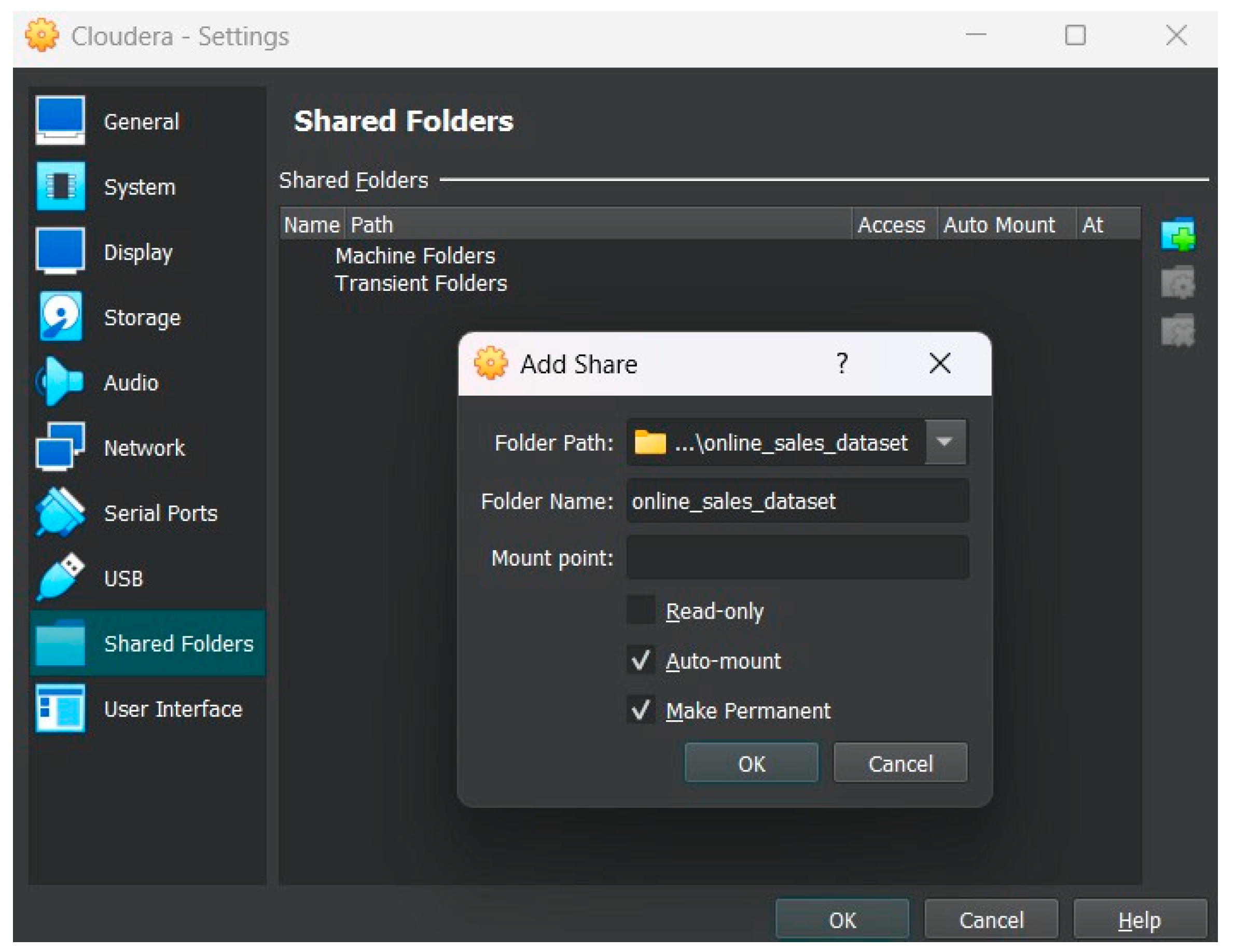
In this step, we are going to create a shared folder in the “Machine Folders” with the name “online_sales_dataset” and specify where the location of the folder path is in Windows. Both “Auto-mount” and “Make Permanent” should be included to avoid mounting the folder every time we reboot the machine and making it permanent to not create a new folder every time.

Figure 5. the “online_sales_dataset” shared folder is created but 1 more step left to do.

Figure 5. the “online_sales_dataset” shared folder is created but 1 more step left to do.

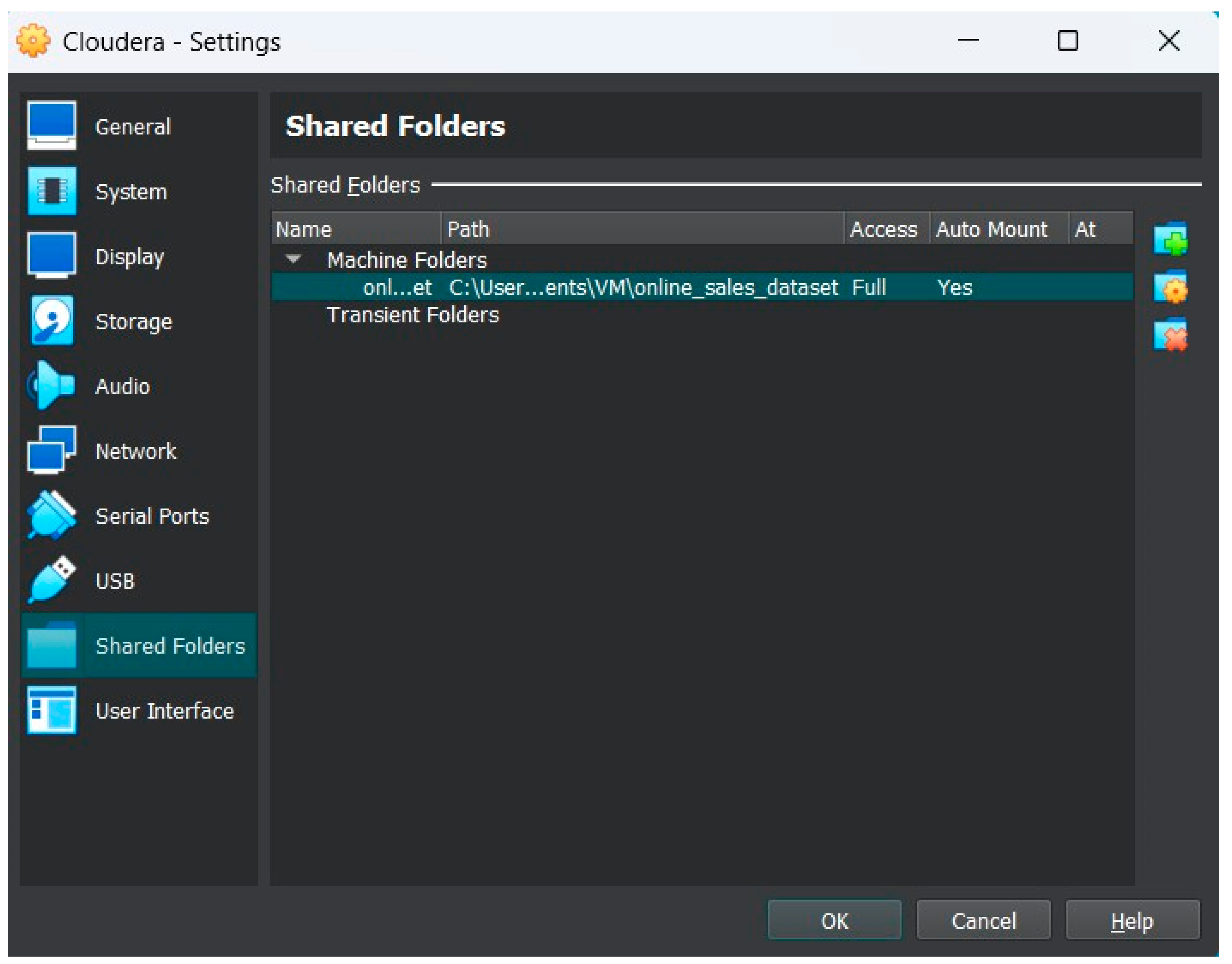
Figure 6. Mounting the shared folder.

Figure 6. Mounting the shared folder.

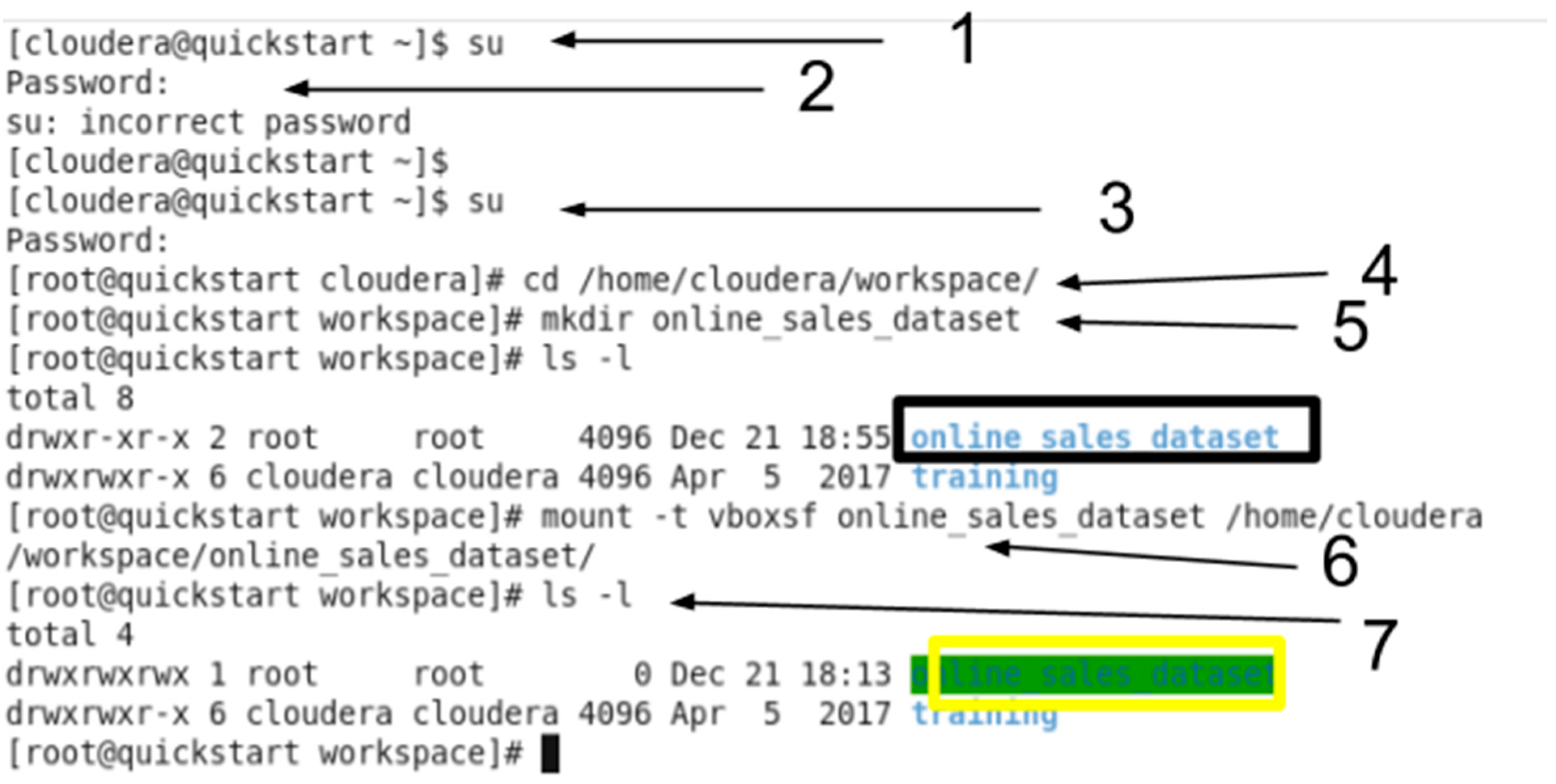
In this step, we should mount the folder after starting Cloudera VM and open the terminal.

• “su” switch user. We login in the terminal as root which has different privileges to mount the desired folder.
• The password is “cloudera”.
• After logging in as the root account, we want to change the directory to this directory “/home/cloudera/workspace/” to add the shared folder.
• We made a directory under the name “online_sales_dataset”.
• We want to list all the directories in “workspace” by using “ls”
• After checking that the directory is created, we want to mount the folder “online_sales_dataset” into this path “/home/cloudera/workspace/online_sales_dataset” to access the shared folder.
• We want to check if the directory is mounted, so we list the available directories and we see the directory with green highlight in the cloudera terminal which means it’s successfully mounted. Now we can start using it to import the dataset.

Figure 7. Same folder and file in Windows host and Cloudera Virtual Machine.

Figure 7. Same folder and file in Windows host and Cloudera Virtual Machine.

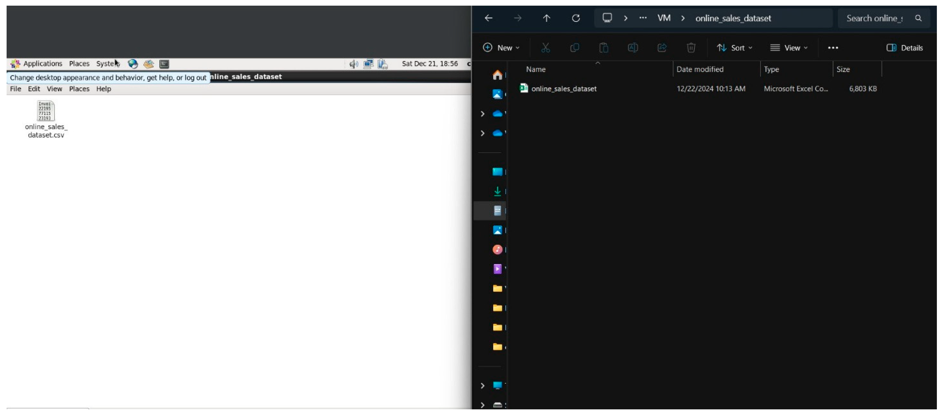
It shows the shared folder in Windows host and Cloudera VM under the same name and have the same file which is the dataset. We can simply add any file in this folder and access it in either Windows host and Cloudera VM.

Figure 8. We displayed the first 10 lines of the dataset to check the dataset file is working as supposed.

Figure 8. We displayed the first 10 lines of the dataset to check the dataset file is working as supposed.

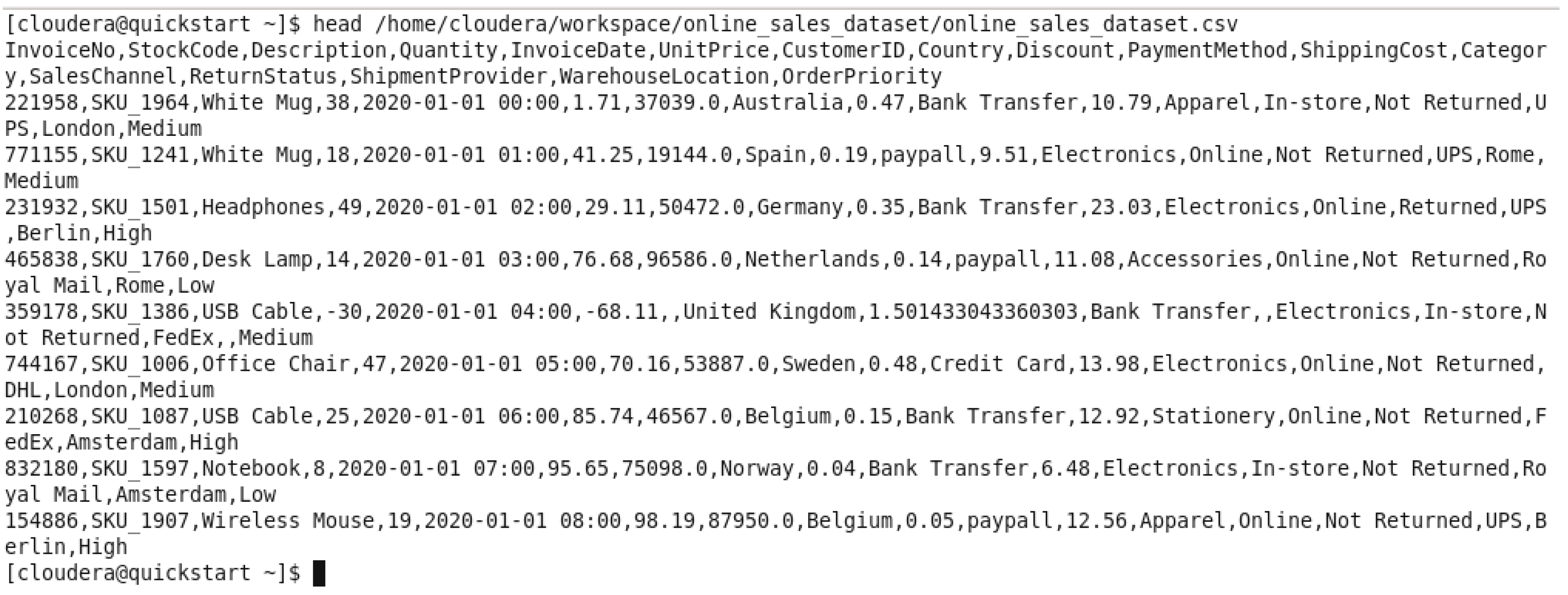
Figure 9. Directory Creation in HDFS.

Figure 9. Directory Creation in HDFS.

We are making directory in hadoop HDFS named “online_sales_dataset” in “/user”/hive/warehouse/’, and the put the dataset file “/home/cloudera/workspace/online_retail/online_sales_dataset.csv” in the new directory in HDFS “/user/hive/warehouse/online_sales_dataset/”. Then we check the contents “ls” and we can verify the new directory created and the dataset file is in there.

5.2. Hive Employment

In this section, we’ll be implementing/employing Hive technology to derive insights using the dataset and SQL-like queries and compare the performance between this technology and other 2 technologies.

Figure 10. Hive login.

Figure 10. Hive login.

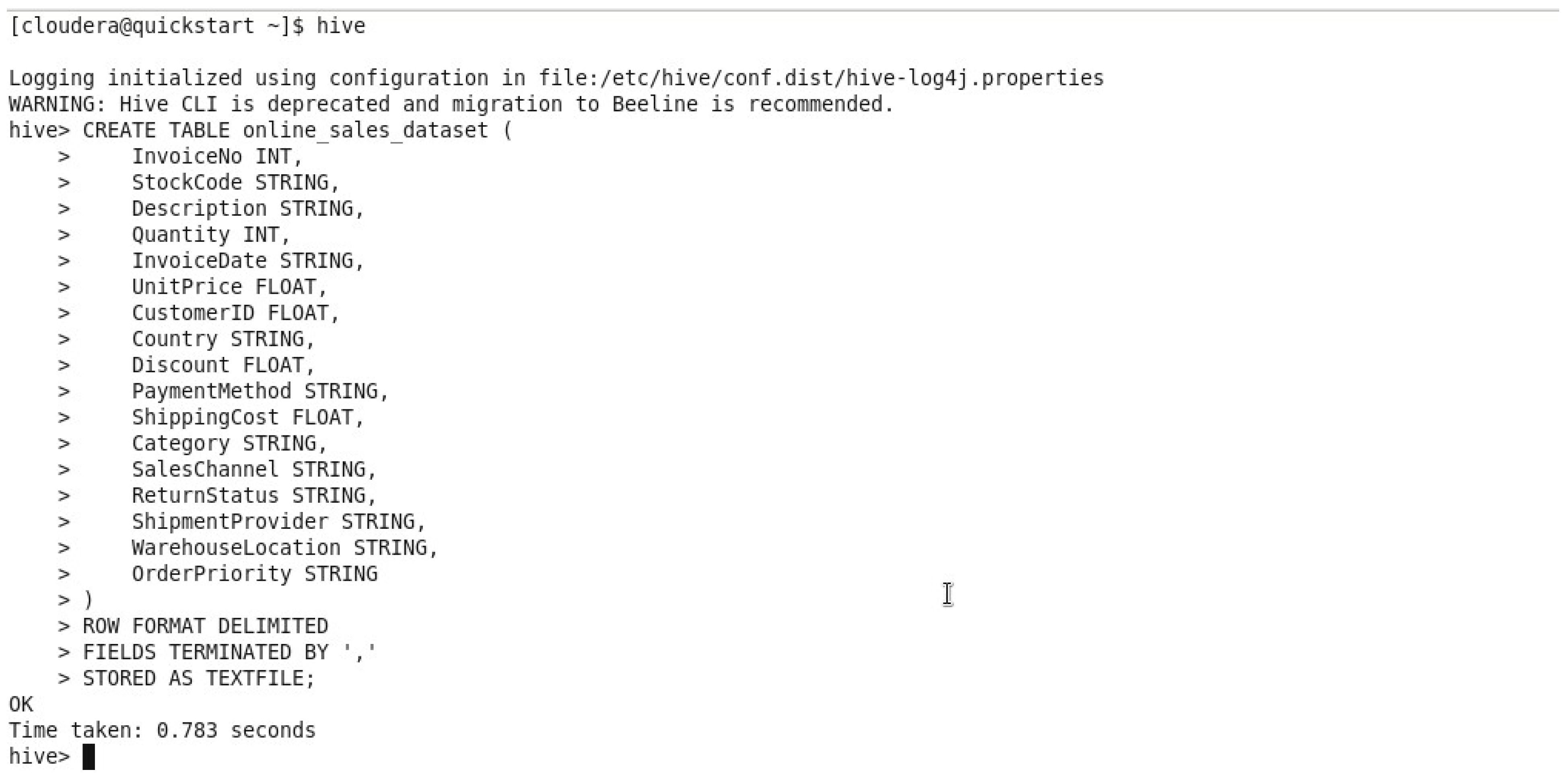
First we log in to hive using cloudera terminal to start importing the dataset to it, after the login we want to CREATE TABLE with the name “online_sales_dataset” to hold the dataset values in it and it has the following attributes and their data types: InvoiceNo INT, StockCode STRING, Description STRING, Quantity INT InvoiceDate STRING, UnitPrice FLOAT, CustomerID FLOAT, Country STRING, Discount FLOAT, PaymentMethod STRING, ShippingCost FLOAT, Category STRING, SalesChannel STRING, ReturnStatus STRING, ShipmentProvider STRING, WarehouseLocation STRING, OrderPriority STRING.

With Apache Hive’s “row format delimited” functionality, fields and lines in a table are terminated using delimiters.

Figure 11. Load dataset into the table.

Figure 11. Load dataset into the table.

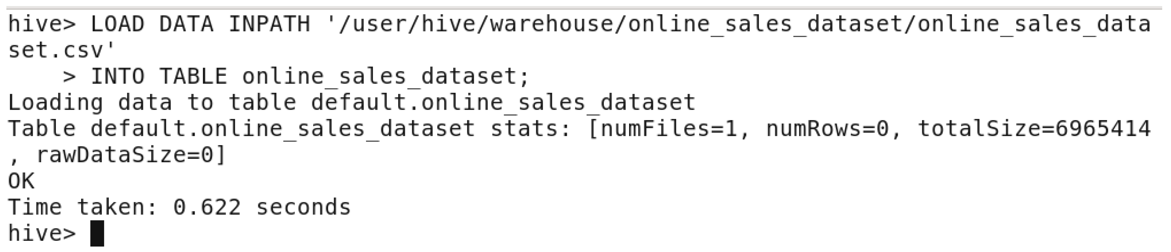
In this step, and after creating the table, we want to LOAD the dataset from where the dataset was stored in this path: “/user/hive/warehouse/online_sales_dataset”. This will load the dataset into the newly created table in figure:

Figure 12. First 20 lines query.

Figure 12. First 20 lines query.

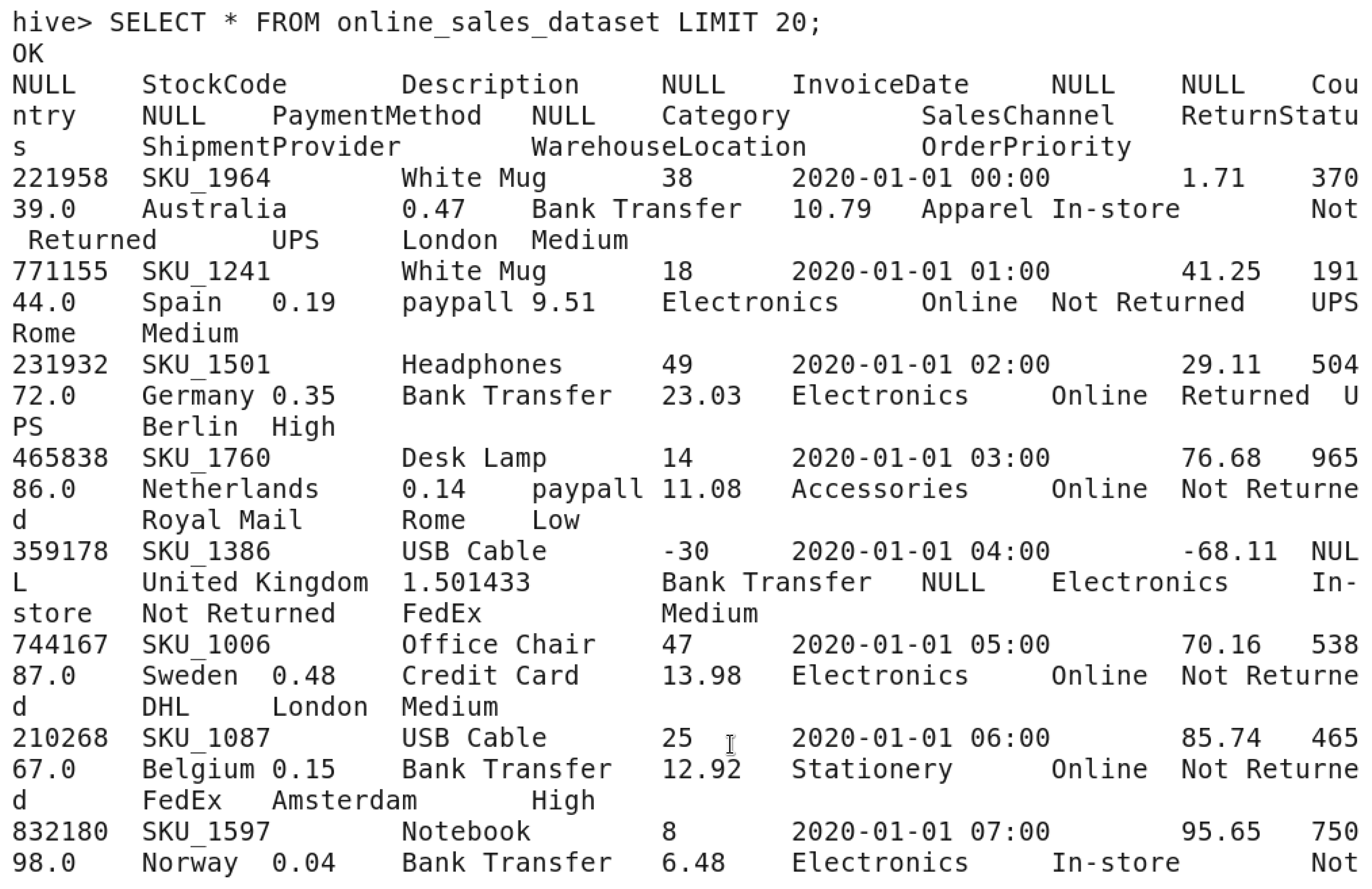
This query is to display the first 20 lines from the table “online_sales_dataset” to check that the table was created and the dataset was loaded without any issues.

The following three metrics: time taken for the query to be executed and giving a valid output, the memory utilized while executing the query and the last is the scalability which will figure out how the upscaled dataset by x2 will affect the time taken and the virtual memory utilized.

5.2.1. Time Taken

Figure 13. Top 10 Products by Quantity Sold QUERY.

Figure 13. Top 10 Products by Quantity Sold QUERY.

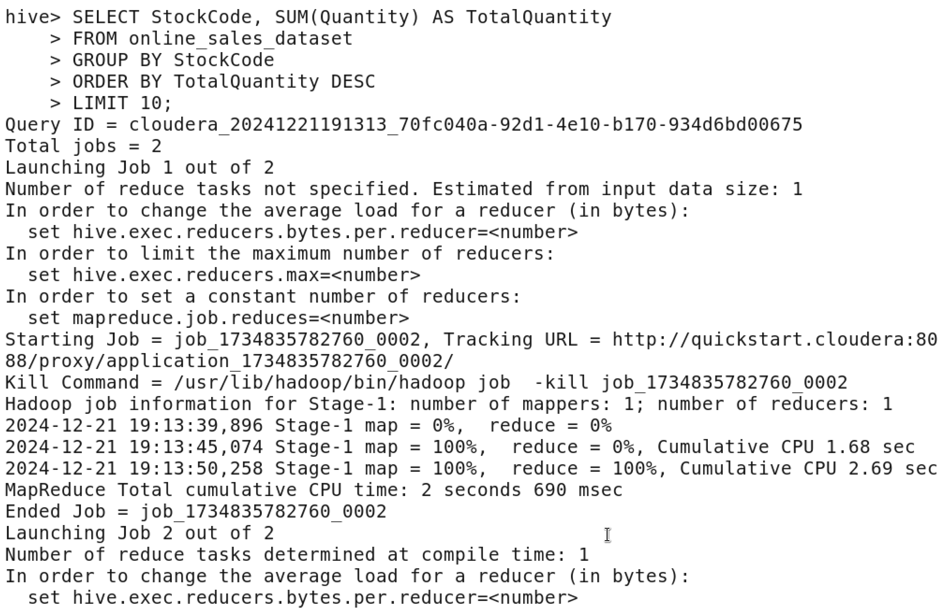
In this figure, we wanted to display the results of the top 10 products by the quantity sold and the time taken to finish this query.

Figure 14. Top 10 Products by Quantity Sold OUTPUT.

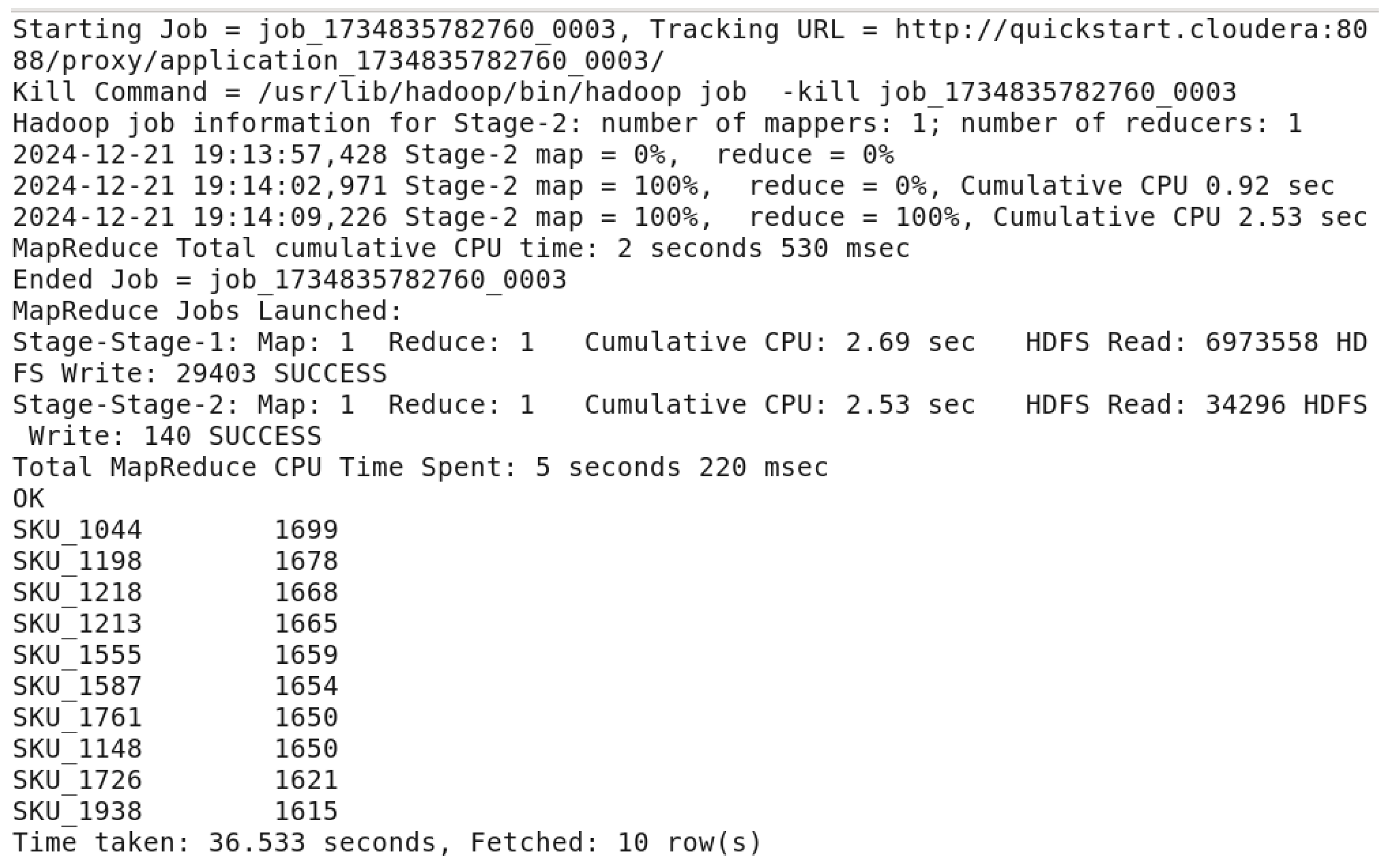
Figure 14. Top 10 Products by Quantity Sold OUTPUT.

After executing the query, we got the output as expected which has the top 10 products sorted by their code and the sum of the quantity. The time taken in total to fetch 10 rows was 39.911 seconds.

5.2.2. Virtual Memory Utilization

A reminder of the assigned random access memory to the virtual machine was 6,144 mb.

Figure 15. Virtual Memory Utilization BEFORE running any query.

Figure 15. Virtual Memory Utilization BEFORE running any query.

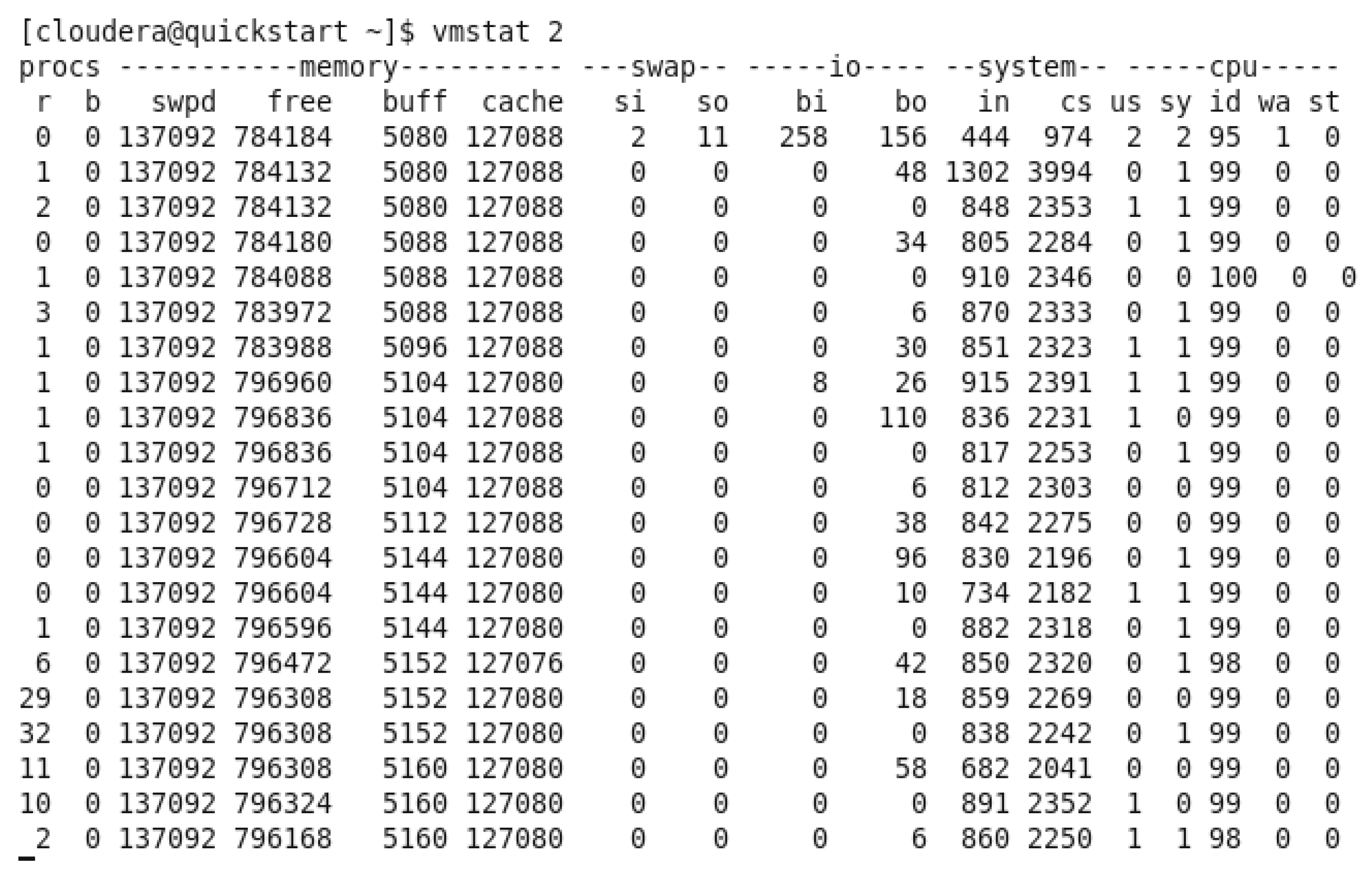
In the previous figure, we can observe the free memory available in the virtual machine before running any query, the avg of the free memory was around 790,382 kb

Figure 16. Top 10 Products by Quantity Sold Virtual Memory Utilization while running the query.

Figure 16. Top 10 Products by Quantity Sold Virtual Memory Utilization while running the query.

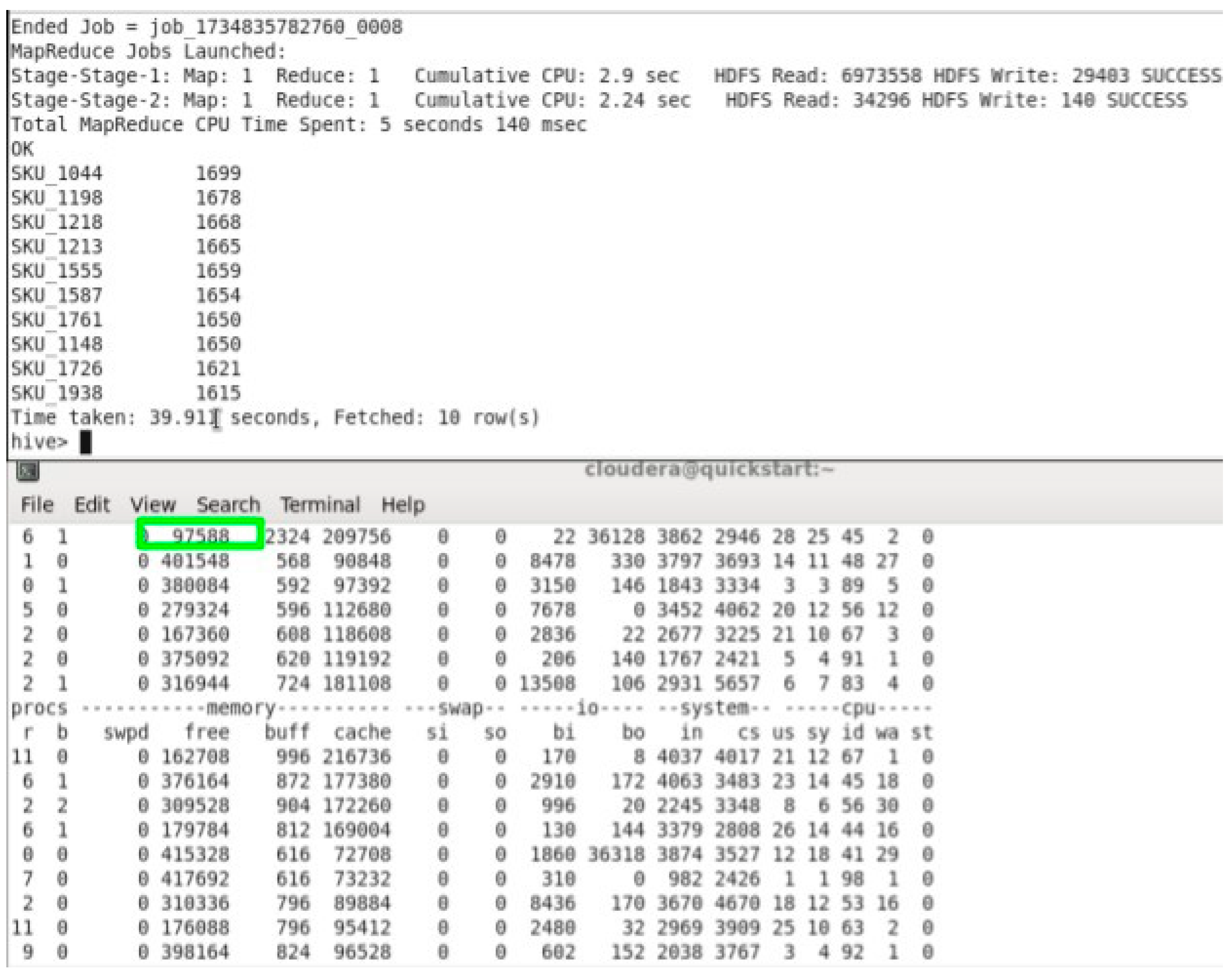
The free memory available when we ran the query achieved the lowest at 97,588 kb. Which is clearly noticeable by hive since it’s considered to be using the most memory.

5.2.3. Scalability

In this metric, what we are going to do is see how scaling up the dataset to a bigger size will affect the time taken to execute queries and memory utilization while execution.

Figure 17. Upscaling the dataset by x2.

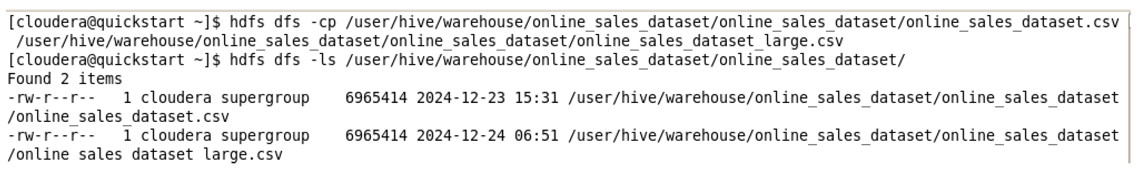
Figure 17. Upscaling the dataset by x2.

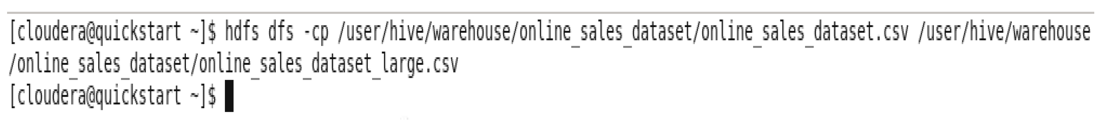
By copying the dataset to itself and saving the bigger dataset under the name “online_sales_dataset_large” in HDFS.

Figure 18. Load the larger dataset into Hive.

Figure 18. Load the larger dataset into Hive.

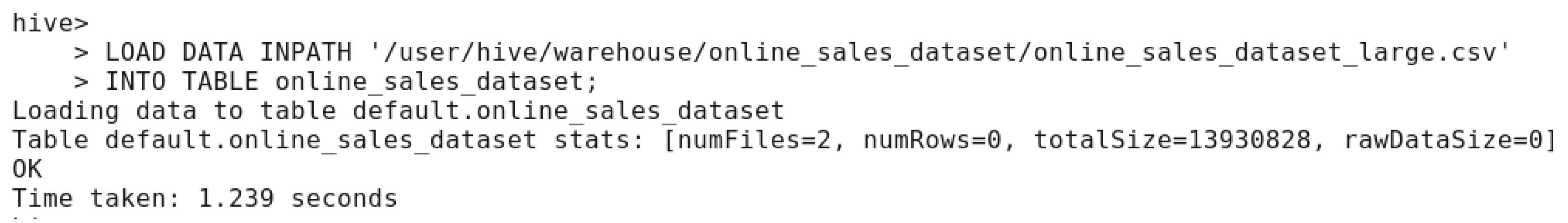
What is done here is loading the upscaled dataset which was saved under the name “online_sales_dataset_large” in the path ‘/user/hive/warehouse/online_sales_dataset/online_sales_dataset_large.csv’ INTO the same table used before which holds the previous dataset.

After that, we will rerun the same query and compare execution time and memory usage for the larger dataset.

1.

Time Taken

Figure 19. Upscaled dataset time taken and memory utilization.

Figure 19. Upscaled dataset time taken and memory utilization.

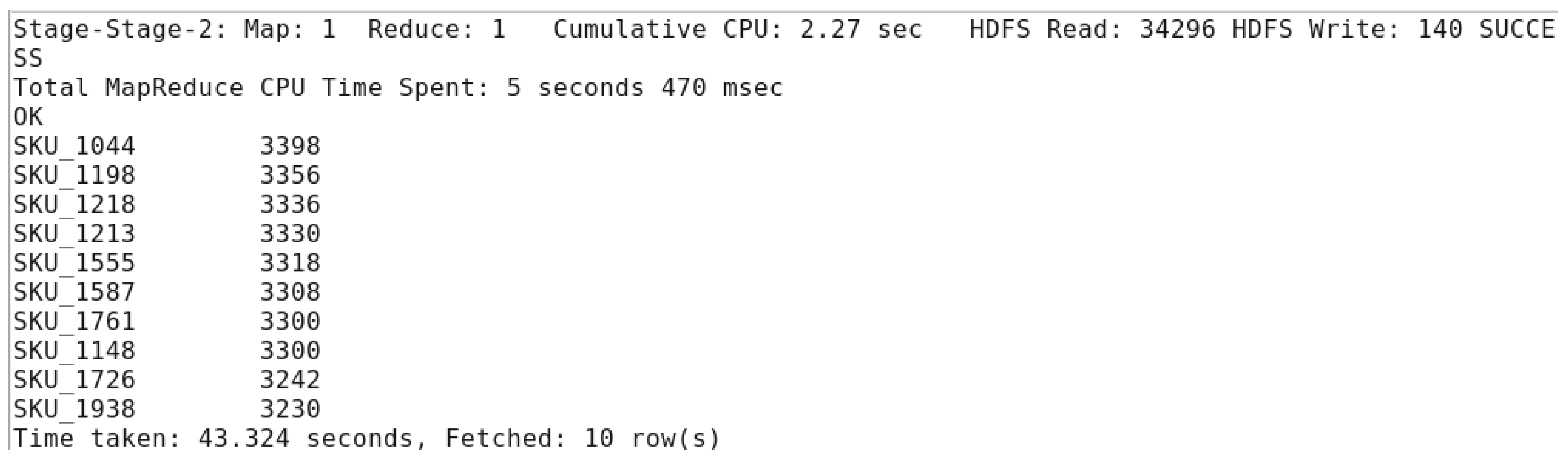
As we can see in the previous figure, the time taken has increased from 39.911 seconds to 43.324 seconds.

2.

Virtual Memory Utilization:

Figure 20. Virtual memory utilization while running Top 10 products by quantity sold on the larger dataset.

Figure 20. Virtual memory utilization while running Top 10 products by quantity sold on the larger dataset.

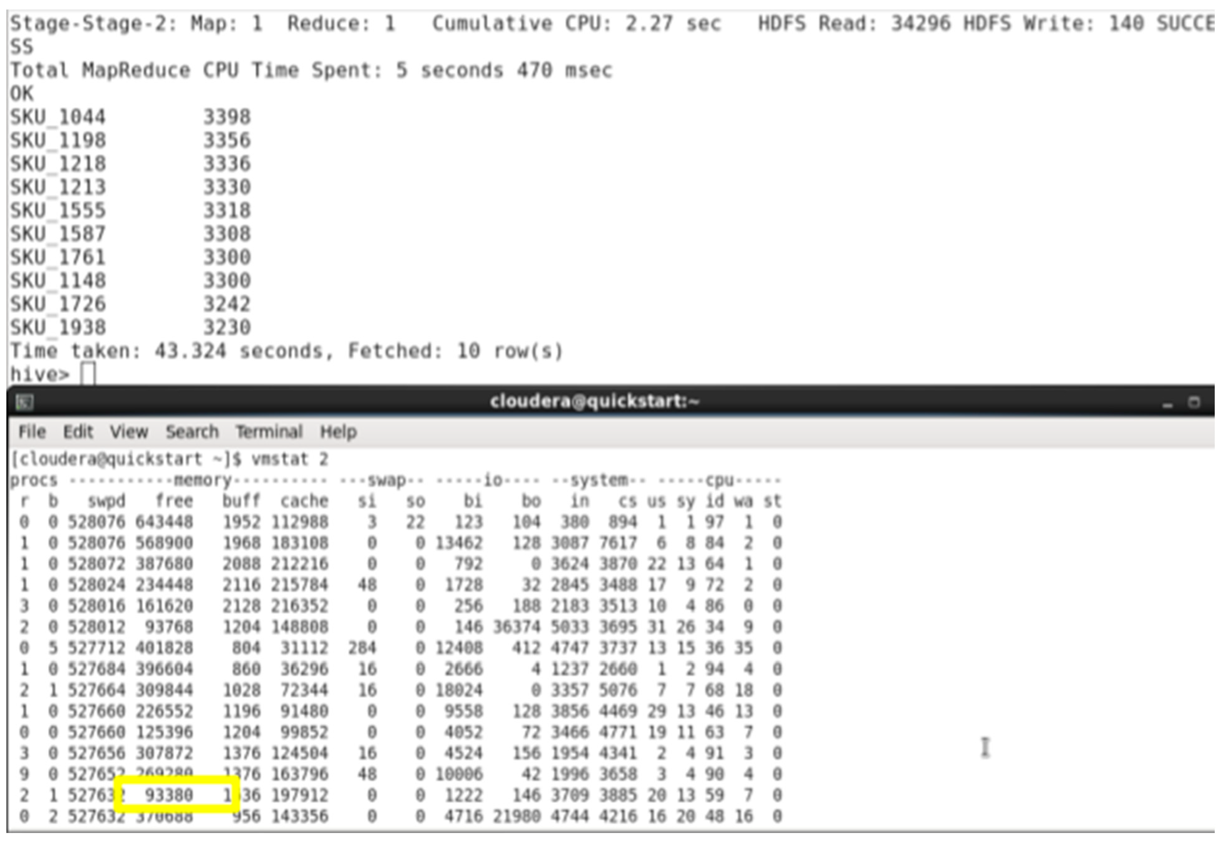
As expected, hive is using more memory in the upscaled dataset than the original dataset before while executing the query to get the top 10 products, free memory reaching the edge be 93,380 kb.

5.3. IMPALA Employment

Figure 21. login to impala shell.

Figure 21. login to impala shell.

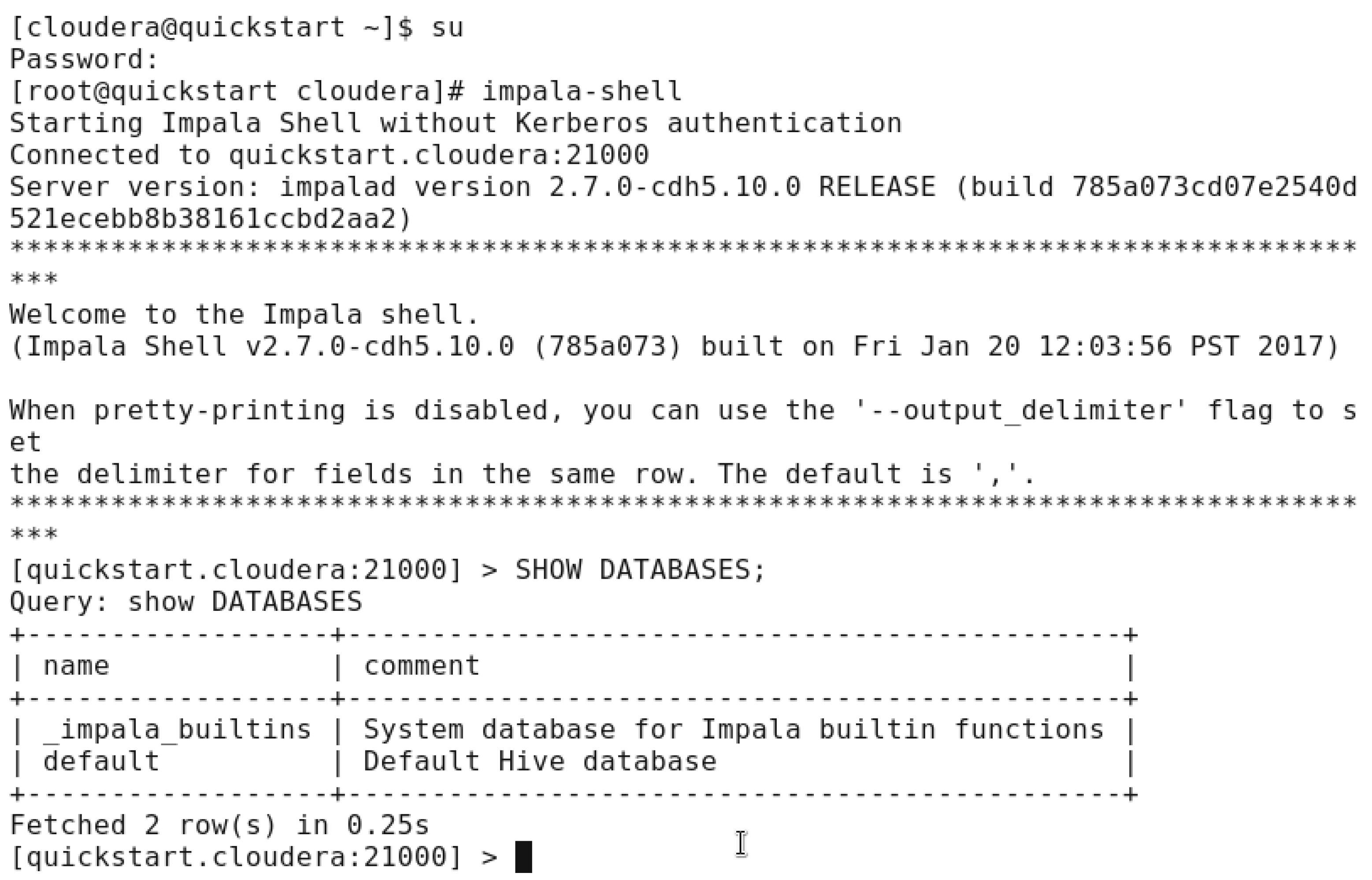
In the previous figure, we started the cloudera terminal and login as root, after that we used “impala-shell” command to access the shell and start employing this technology on the dataset we have. The available databases have been displayed using “SHOW DATABASES” and we clearly see only 2 databases available.

Figure 22. location of the dataset in HDFS.

Figure 22. location of the dataset in HDFS.

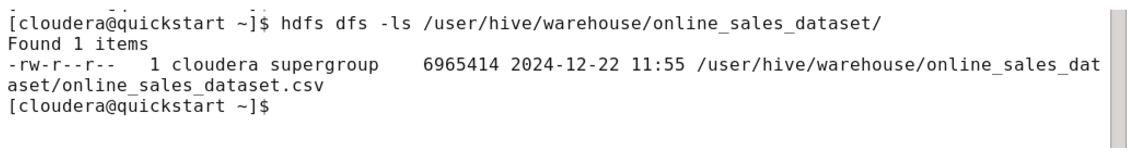
In this figure, we already have the dataset imported to HDFS and there is no need to put it again from the shared folder.

Figure 23. Showing available databases.

Figure 23. Showing available databases.

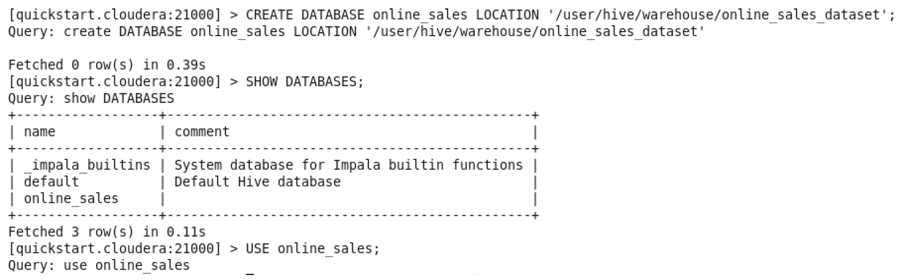
In this step, we created a new database called “online_sales” and the location of it was in this path ‘/user/hive/warehouse/online_sales_dataset’, displayed the available databases and put the newly created one to be used by the command “USE online_sales”.

Figure 24. Table creation in the database.

Figure 24. Table creation in the database.

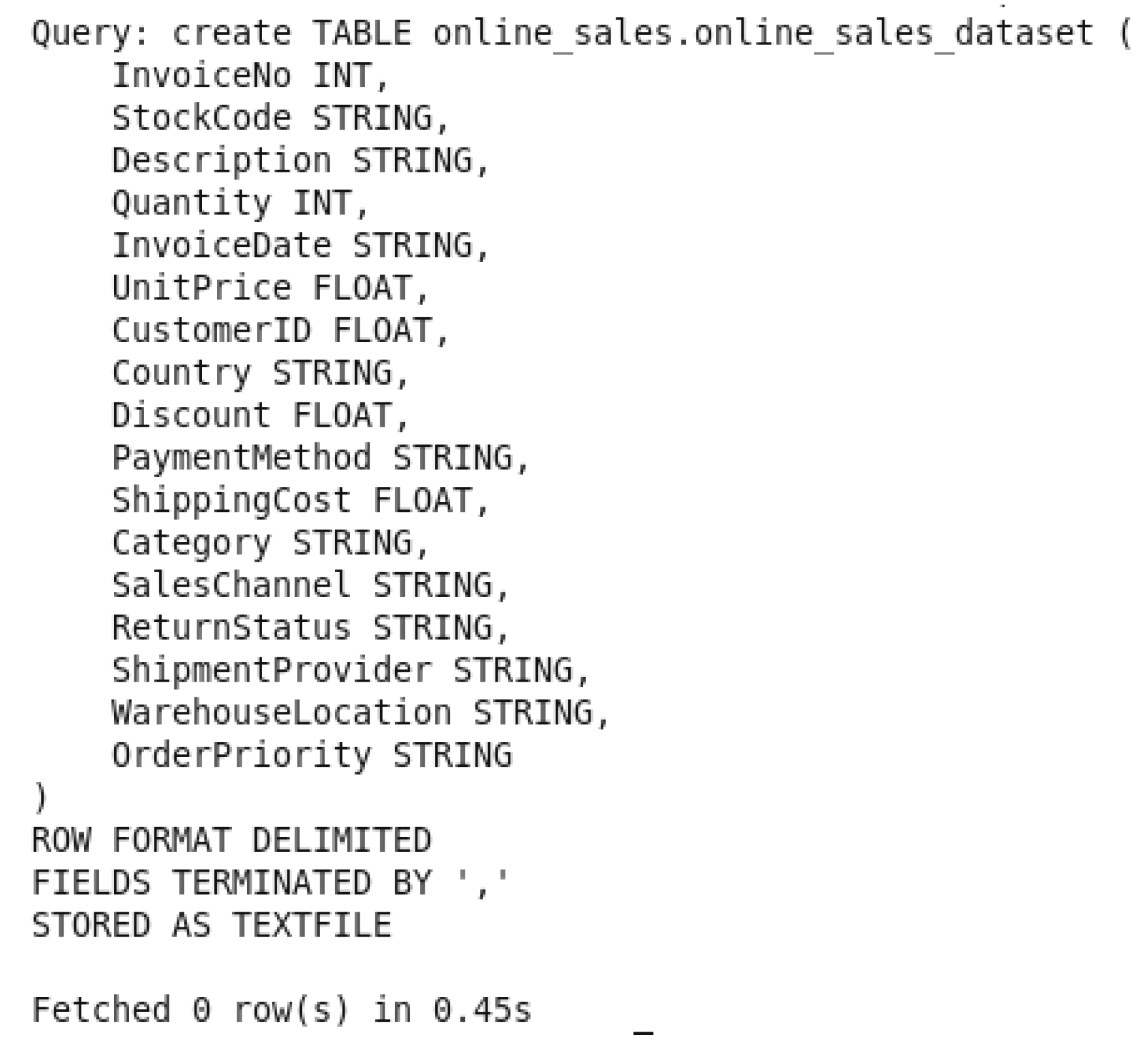
In this step, and after creating the database, we created the table “online_sales_dataset” in the database “online_sales”.

Figure 25. Displaying the available tables in th database.

Figure 25. Displaying the available tables in th database.

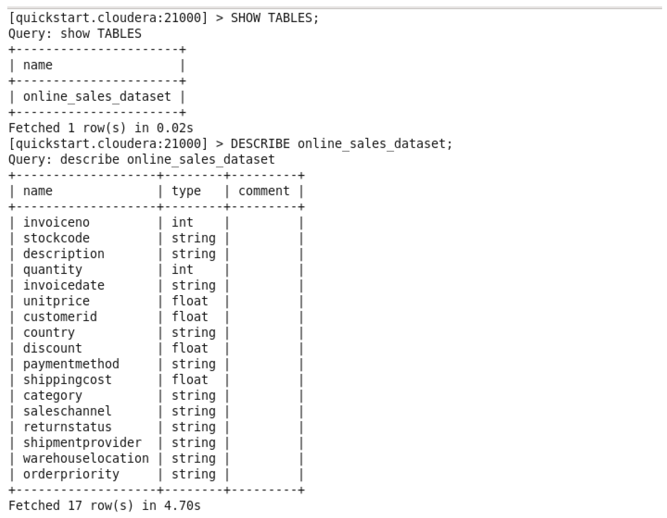
In this figure, there are 2 commands, one to show the available tables created, and to describe an available table and in our case it’s “online_sales_dataset” which means verifying the attributes and data types of the table.

Figure 26. Load dataset into the table.

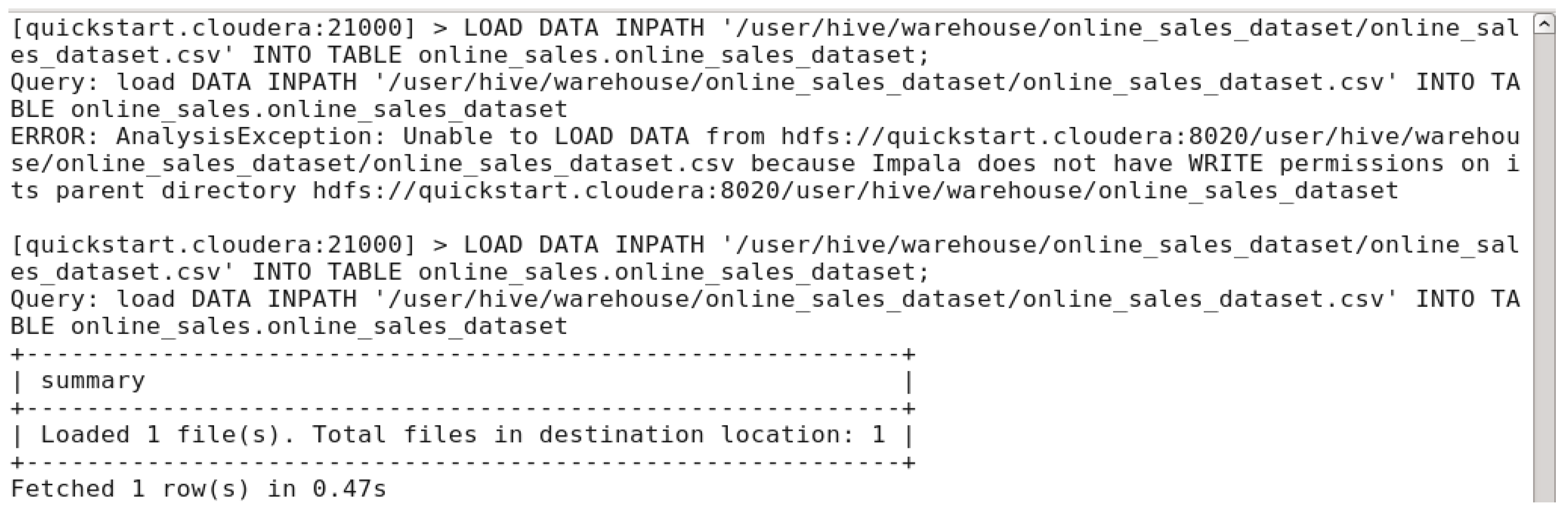
Figure 26. Load dataset into the table.

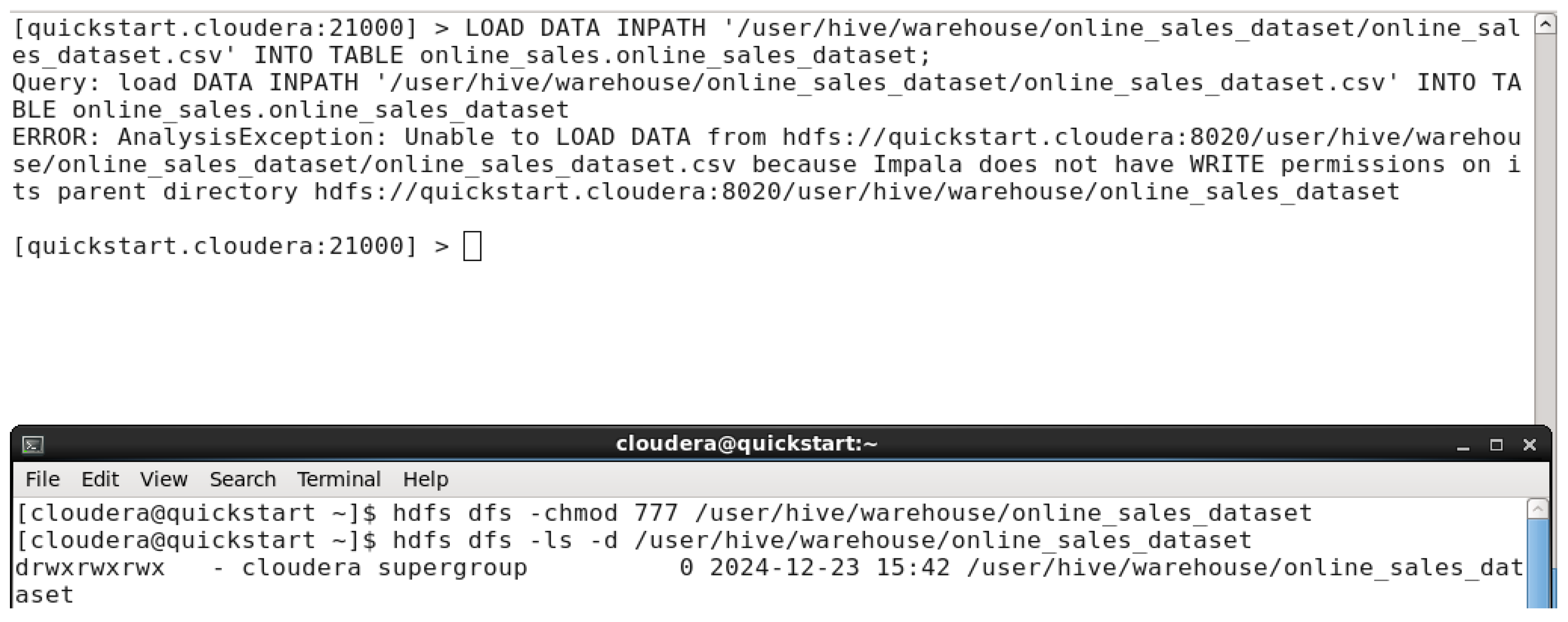
In this step, we tried to load the dataset into the created table but an error showed up requiring impala the permission to be able to write on the parent directory. By using a command in another

cloudera terminal ‘hdfs dfs -chmod 777 /user/hive/warehouse/online_sales_dataset’. In the next figure we’ll be able to load the dataset into the table.

Figure 27. Dataset loaded successfully into the table.

Figure 27. Dataset loaded successfully into the table.

5.3.1. Time Taken

Figure 28. Executing Top 10 Products by Quantity Sold Query.

Figure 28. Executing Top 10 Products by Quantity Sold Query.

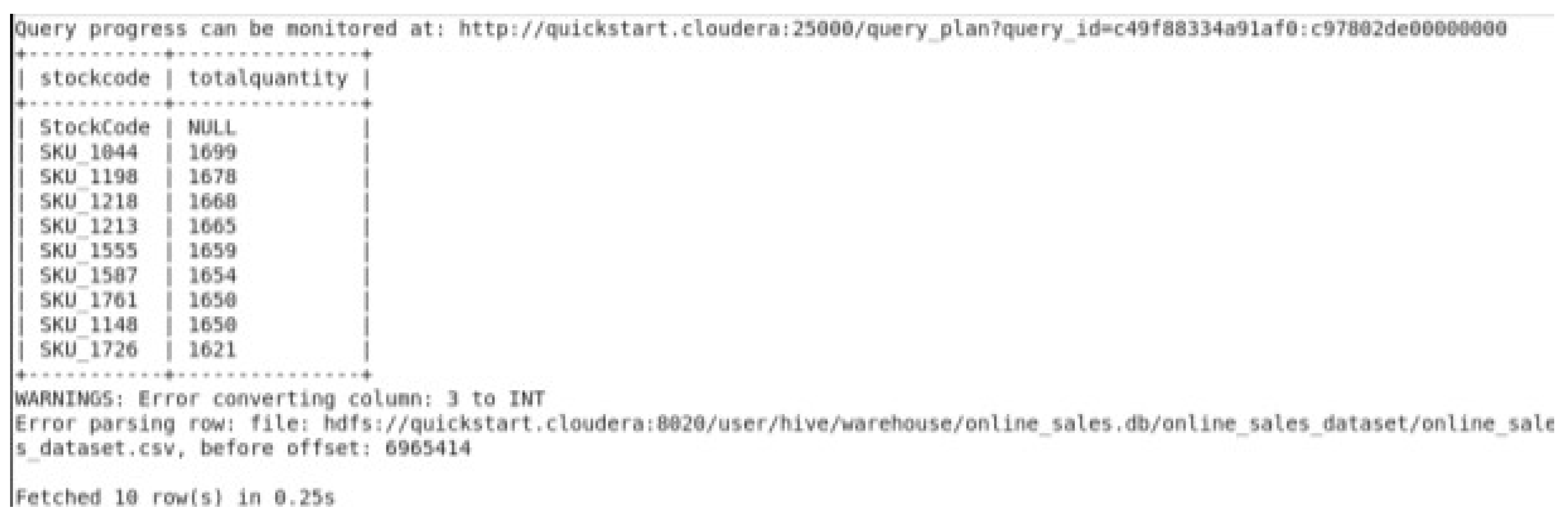
The time taken in the query using impala technology was 0.25 seconds to fetch 10 rows.

5.3.2. Virtual Memory Utilization

Figure 29. Virtual Memory Utilization BEFORE running any query.

Figure 29. Virtual Memory Utilization BEFORE running any query.

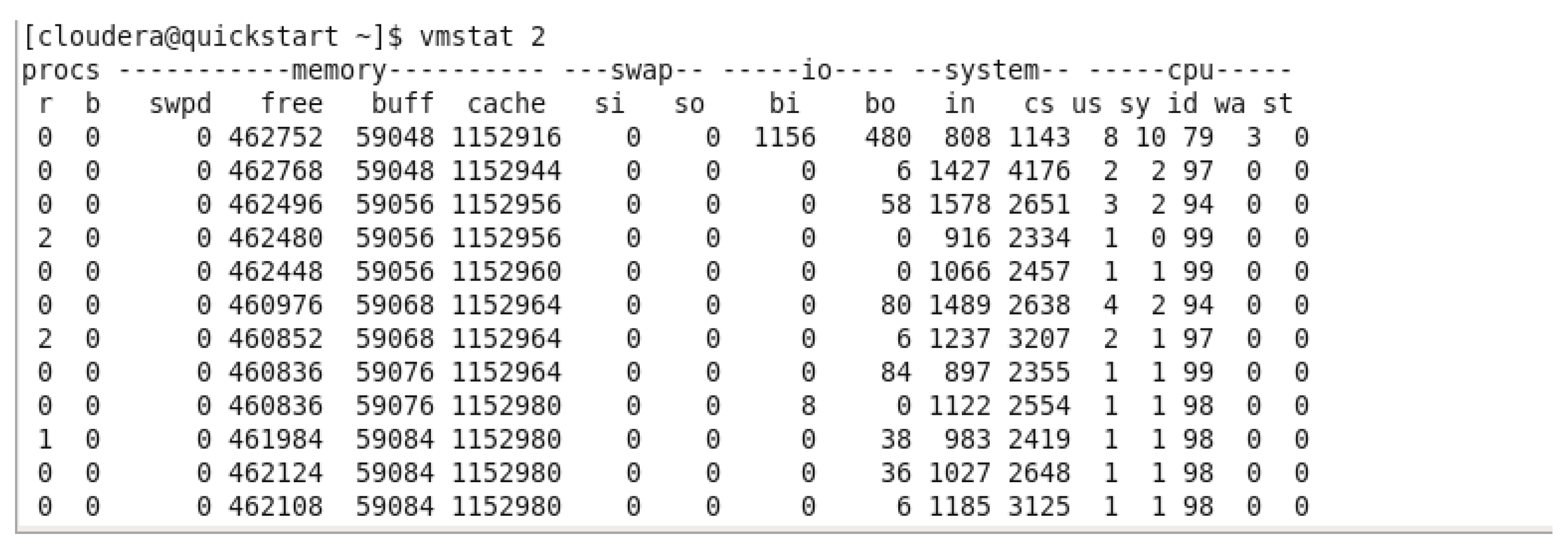
In the previous figure, we can observe the free memory available in the virtual machine before running any query, the avg of the free memory was around 461,418 kb.

Figure 30. Virtual Memory Utilization While running Top 10 Products by quantity sold.

Figure 30. Virtual Memory Utilization While running Top 10 Products by quantity sold.

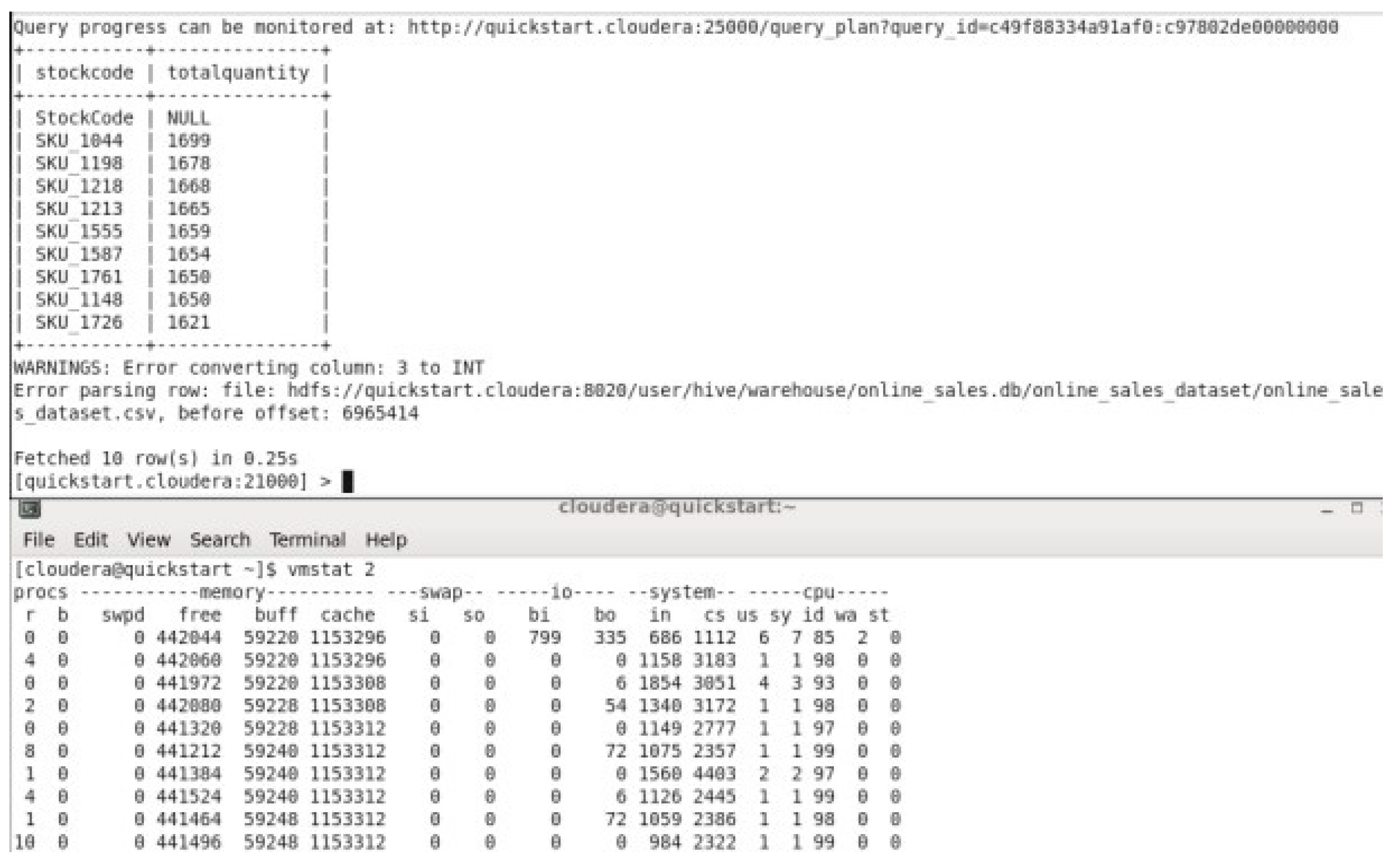
In the previous figure, we can observe the free memory available in the virtual machine while running Top 10 Products by quantity sold , the avg of the free memory was around 441,708 kb.

5.3.3. Scalability

Figure 31. Dataset file duplication.

Figure 31. Dataset file duplication.

The dataset file used in previous query, will be copied to the same directory to have larger dataset, so the original dataset has 49,783 rows and the larger dataset will have x2 the number or the rows in the original one.

Figure 32. Loading upscaled dataset into the table.

Figure 32. Loading upscaled dataset into the table.

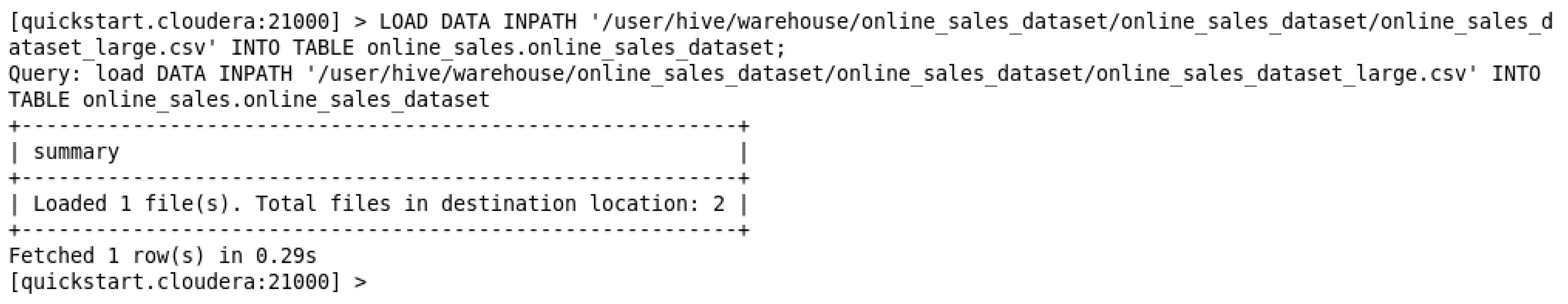
This step, as previous steps, is to simply load the larger dataset into the table in “online_sales” database.

• Time Taken

Figure 33. Time taken for upscaled dataset.

Figure 33. Time taken for upscaled dataset.

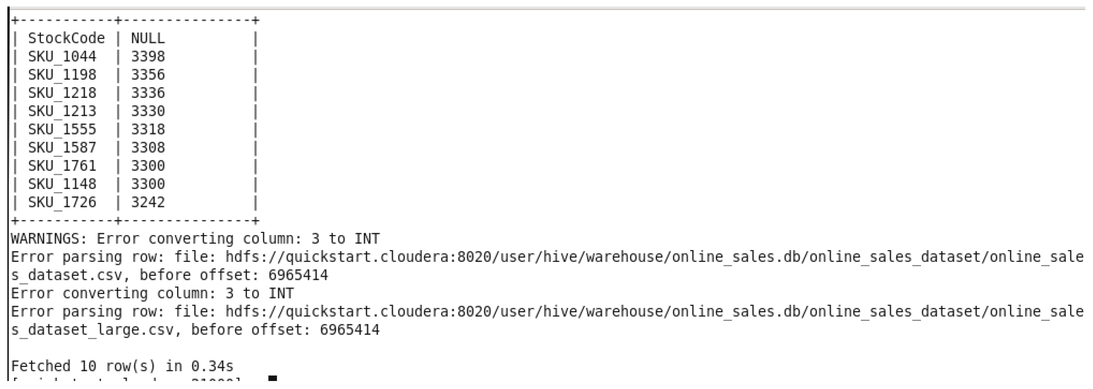
This query has been executed using the large dataset to fetch 10 rows. The 10 rows were fetched in 0.34 seconds. It took around more 0.10 seconds to fetch the rows of the top 10 products than the original dataset.

2.

Virtual Memory Utilization

Figure 34. Virtual Memory Utilization for the upscaled dataset while executing the top 10 products by quantity sold.

Figure 34. Virtual Memory Utilization for the upscaled dataset while executing the top 10 products by quantity sold.

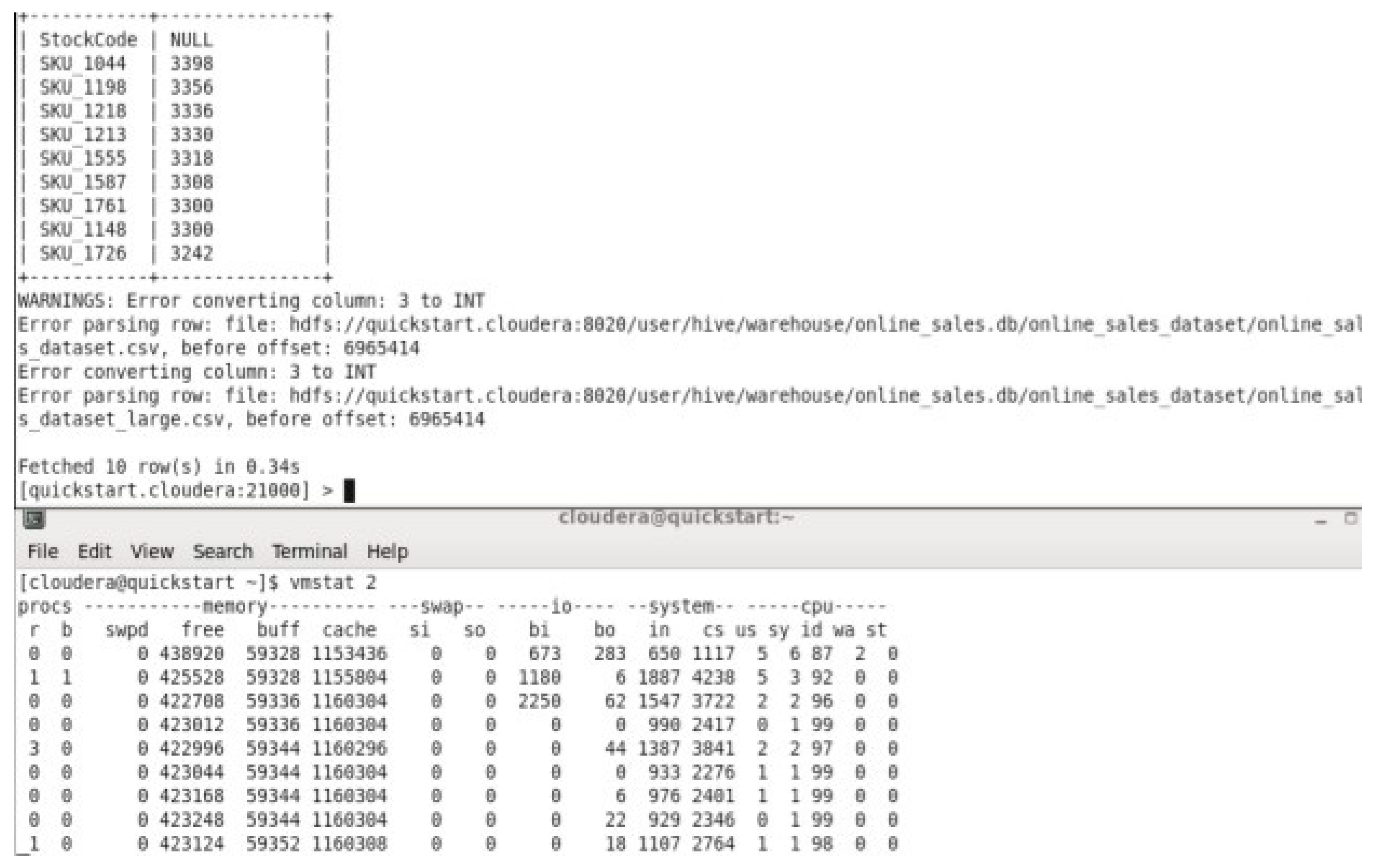
In the previous figure, we can observe the free memory available in the virtual machine while running Top 10 Products by quantity sold on the upscaled dataset, the avg of the free memory was around 423,561 kb which is using more memory than executing the same query on original dataset.

5.4. PIG Employment

Apache Pig is a high-level platform for creating data processing programs that run on Hadoop. It uses a scripting language called Pig Latin, which simplifies the task of analyzing large datasets. Pig translates these scripts into MapReduce jobs, making it an efficient tool for big data analytics. In this project, Pig was employed to perform various analytical operations on the dataset, such as calculating total revenue, identifying top products by sales, analyzing monthly trends, determining the average discount per product category, and calculating total orders by payment method. We chose to demonstrate the execution time using the query for calculating total revenue and memory utilization using the query for identifying top products by sales. All queries were executed in the Pig shell.

Figure 35. Entering the PIG shell.

Figure 35. Entering the PIG shell.

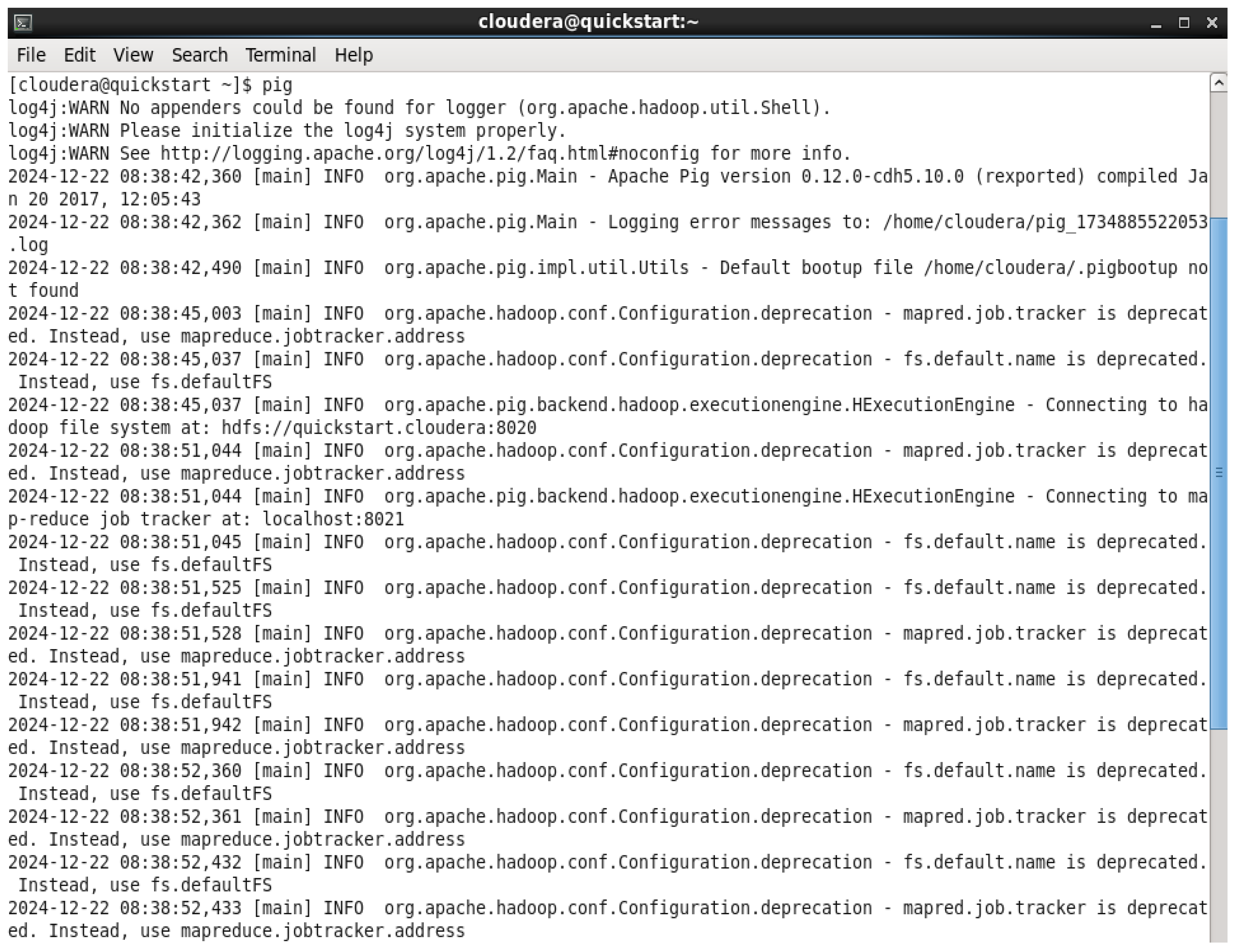
After entering into the pig shell it is compulsory to load the dataset within the pig before running any queries.

Figure 36. Loading the dataset from HDFS.

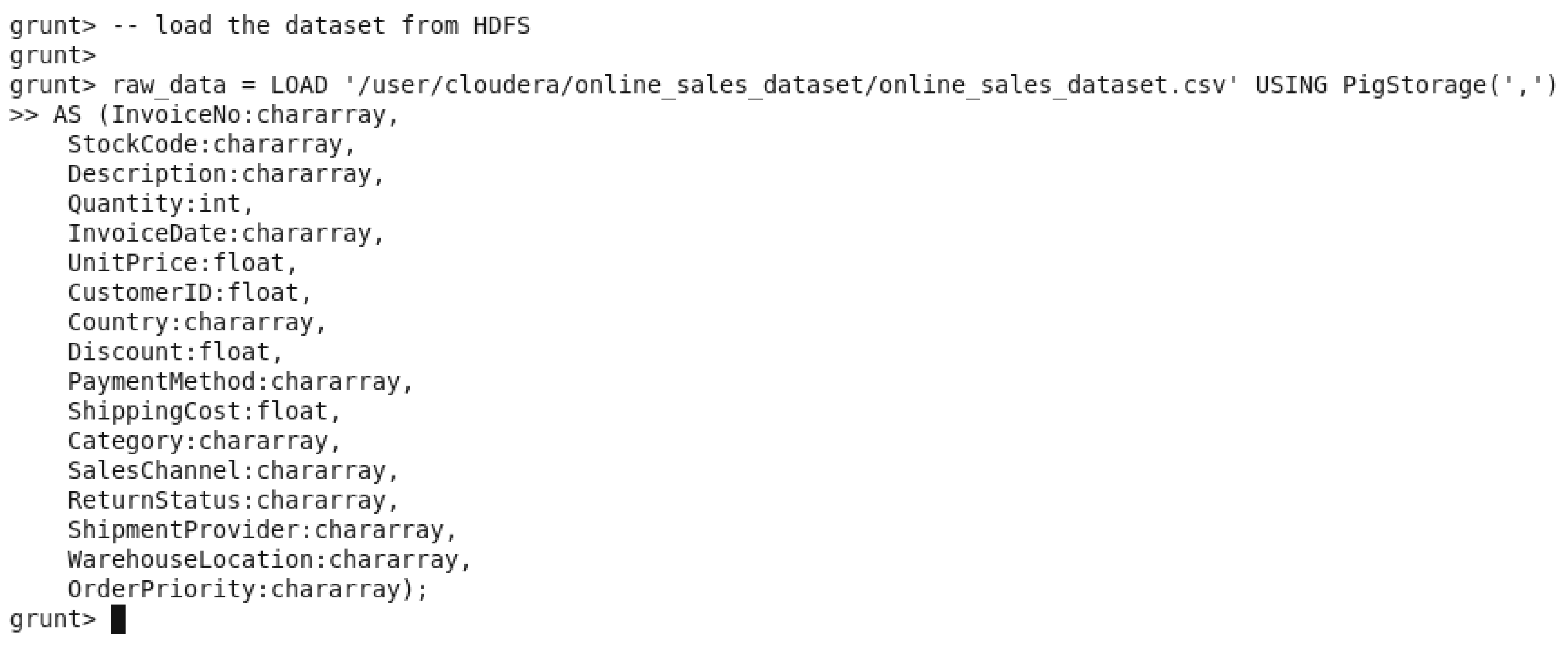
Figure 36. Loading the dataset from HDFS.

5.4.1. Time Taken

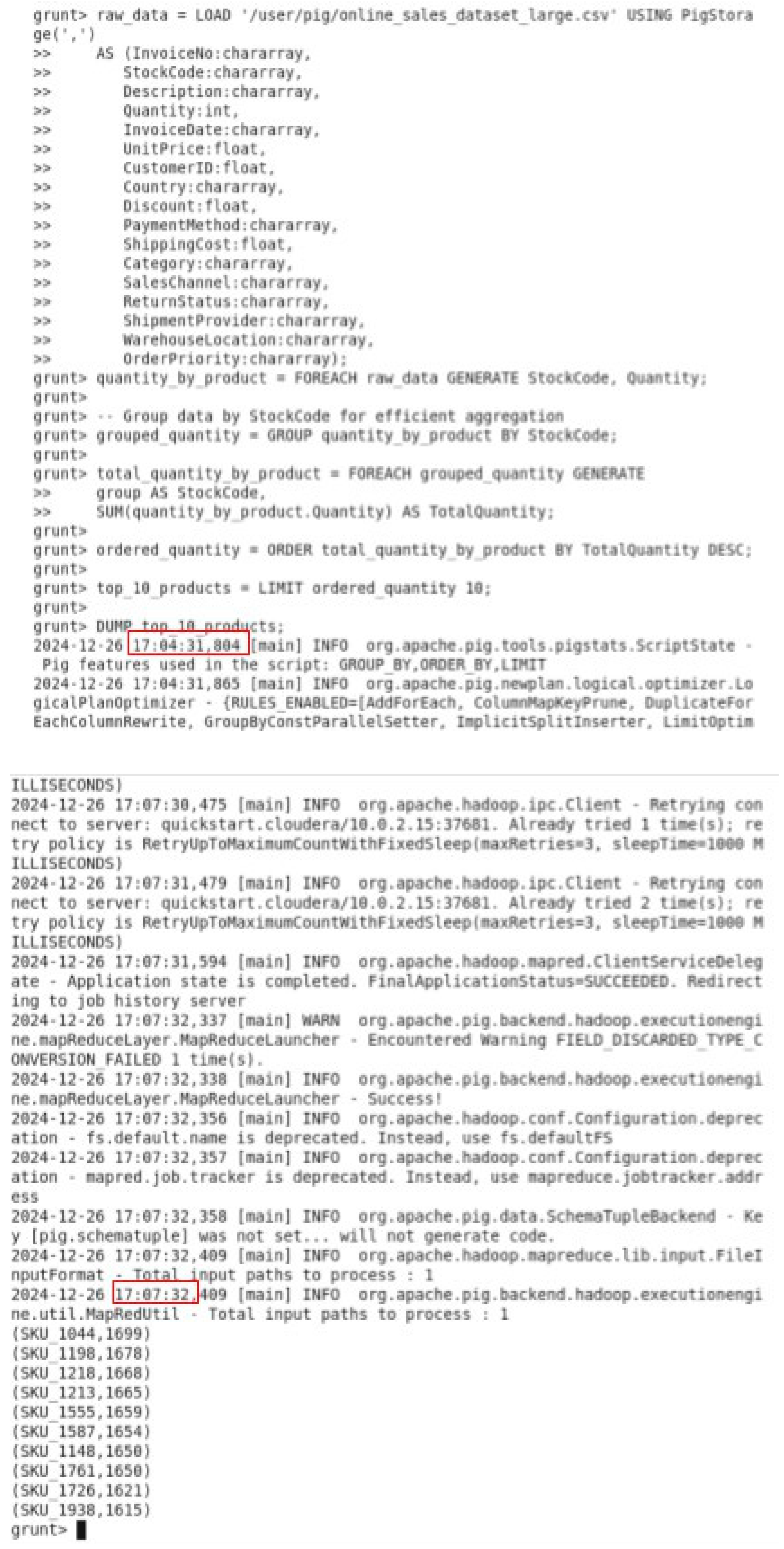
Figure 37. Starting time.

Figure 37. Starting time.

Figure 38. Finishing time.

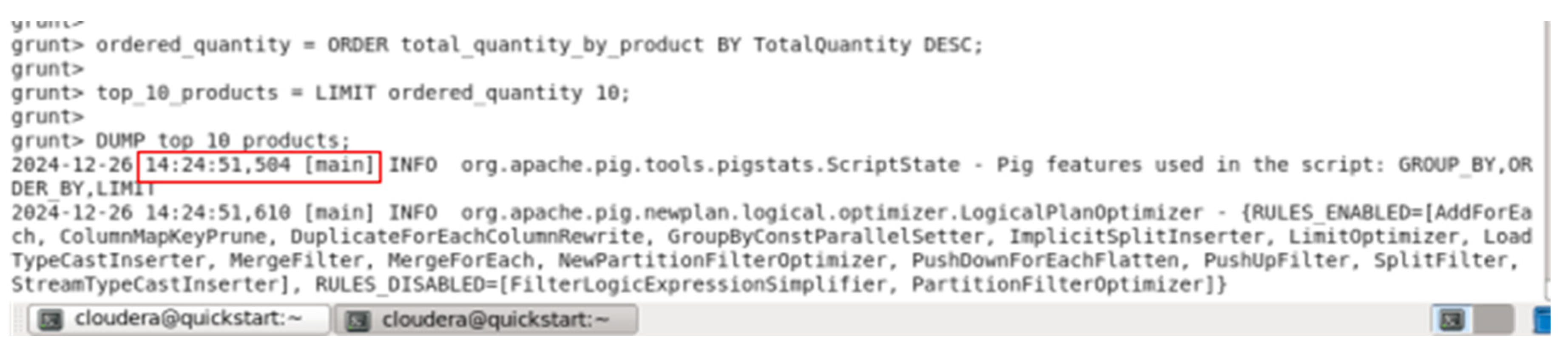
Figure 38. Finishing time.

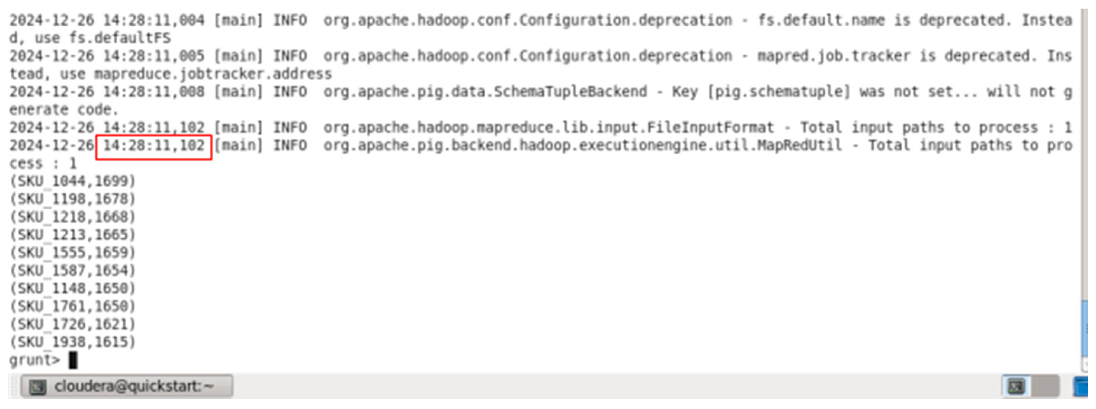
The execution time for the query “Top 10 Products by Quantity Sold” was 3 minutes and 26 seconds. This time reflects the duration required to process the dataset and compute the total quantity sold for each product, followed by ordering the results and limiting the output to the top 10 products. The process involved grouping the data by StockCode, aggregating the Quantity

field, sorting the results in descending order of total quantity sold, and then limiting the result to the top 10 products.

This execution time is a crucial metric, as it demonstrates the efficiency of the query in processing a large dataset containing over 49,000 transaction records, making it suitable for real-time or near-real-time analysis in a retail or e-commerce environment.

5.4.2. Virtual Memory Utilization

The virtual memory utilization during the execution of the “Top 10 Products by Quantity Sold” query on the dataset offers valuable insights into the system’s resource consumption when processing large volumes of data in Pig.

Figure 39. Before running Top 10 Products by Quantity Sold.

Figure 39. Before running Top 10 Products by Quantity Sold.

Figure 40. Top 10 Products by Quantity Sold VMU WHILE RUN.

Figure 40. Top 10 Products by Quantity Sold VMU WHILE RUN.

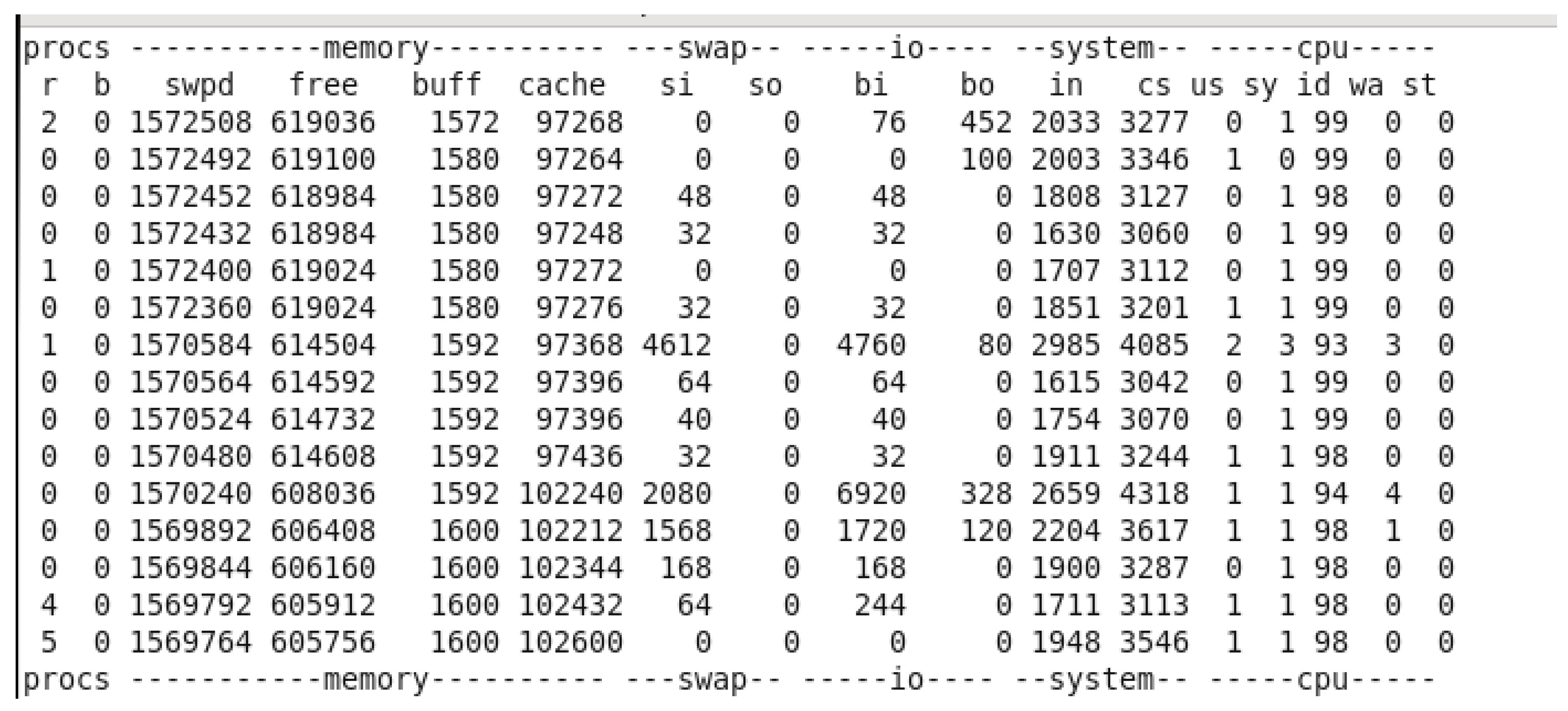
Figure 41. After finishing and query and closing terminal.

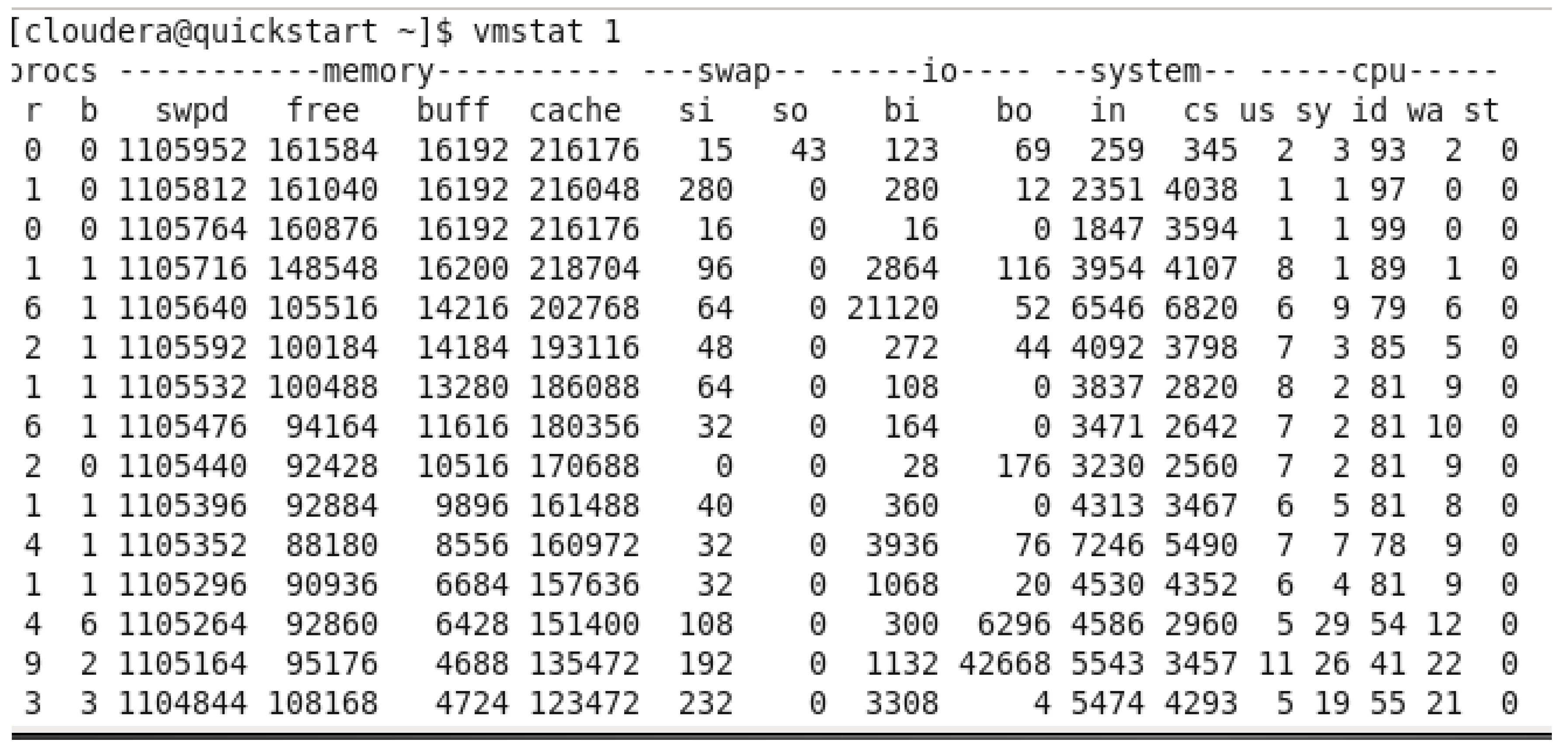
Figure 41. After finishing and query and closing terminal.

Initially, before running the query, the system had 619,063 KB of free memory. However, as the query was executed, the memory utilization increased, causing the free memory to decrease significantly, reaching its lowest point at 88,180 KB. This decline in available memory can be attributed to the processing load involved in aggregating and sorting a large number of records, particularly given the substantial size of the dataset with over 49,000 transactions. After the query execution was completed and the terminal was closed, the system’s free memory returned to its maximum value of 978,056 KB, suggesting that resources were efficiently freed up. This fluctuation in virtual memory utilization highlights the system’s memory demands during intensive data operations and the need for effective resource management when running large-scale queries in Pig.

5.4.3. Scalability

Figure 42. Enlarging Dataset.

Figure 42. Enlarging Dataset.

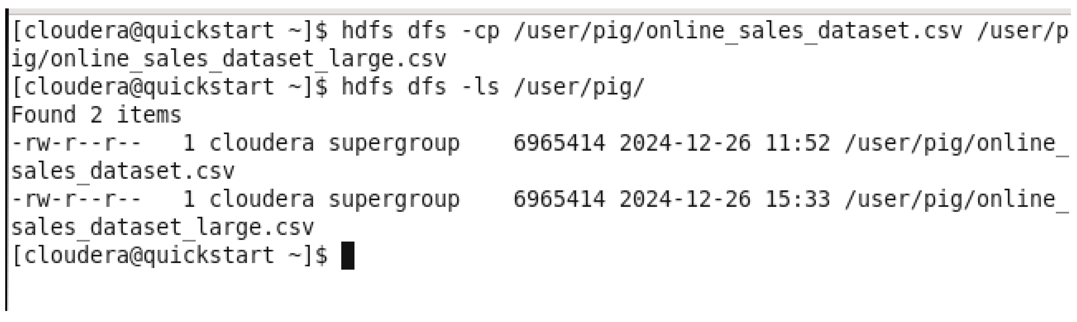
Here we have upscaled the dataset by just copying the older dataset and using large.csv.

1.

Time Taken: The execution time for the query “Top 10 Products by Quantity Sold” was 3 minutes 31.32 seconds.

Figure 43. Upscaled Datasets Output for Top 10 Products by Quantity Sold.

Figure 43. Upscaled Datasets Output for Top 10 Products by Quantity Sold.

This will give the time taken for processing the enlarged dataset and calculating the total quantity sold for every product, ordering the result, and showing only the top 10 products. This involved grouping the data by StockCode, summing up the Quantity field, sorting the results in descending order of total quantity sold, and then limiting the result to the top 10 products.

This execution time is one of the most important metrics, since it shows how well the query scales for an upscaled larger dataset with more than 49,000 transaction records, thus making it suitable for real-time or near-real-time analysis in a retail or e-commerce environment.

2.

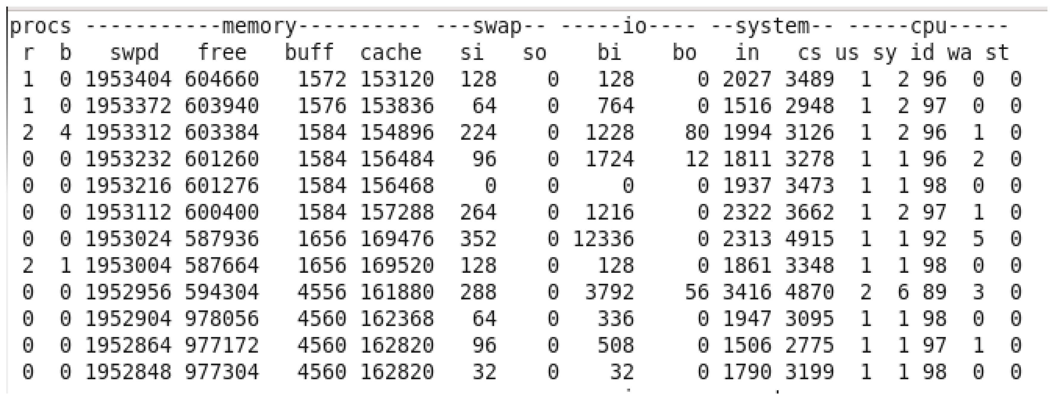
VMU : Virtual memory used by the “Top 10 Products by Quantity Sold” query, when executed on the larger dataset, gives an idea about how the system consumes resources to process a large volume of data in Pig.

Figure 44. VMU before running the query.

Figure 44. VMU before running the query.

Figure 45. While running the query.

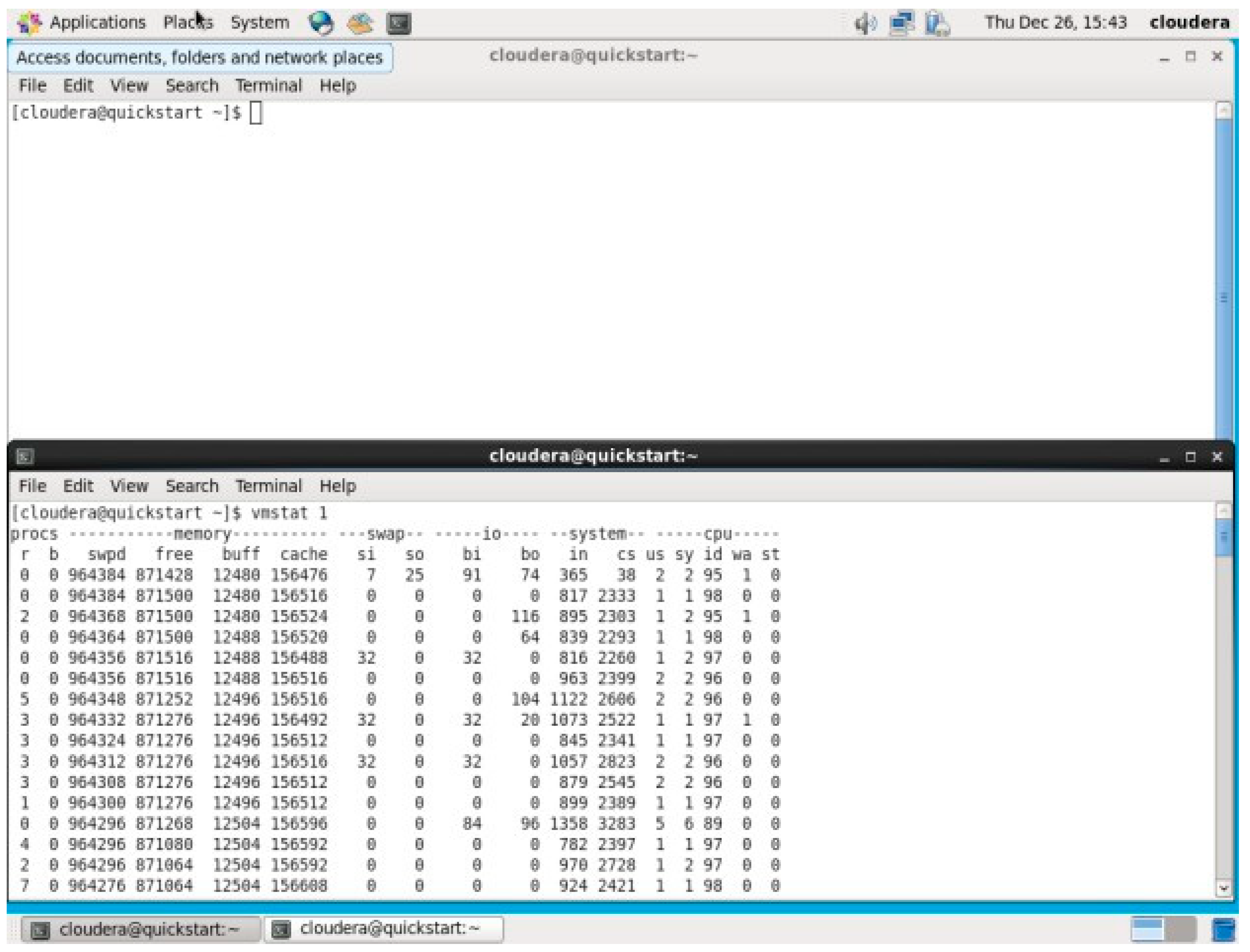
Figure 45. While running the query.

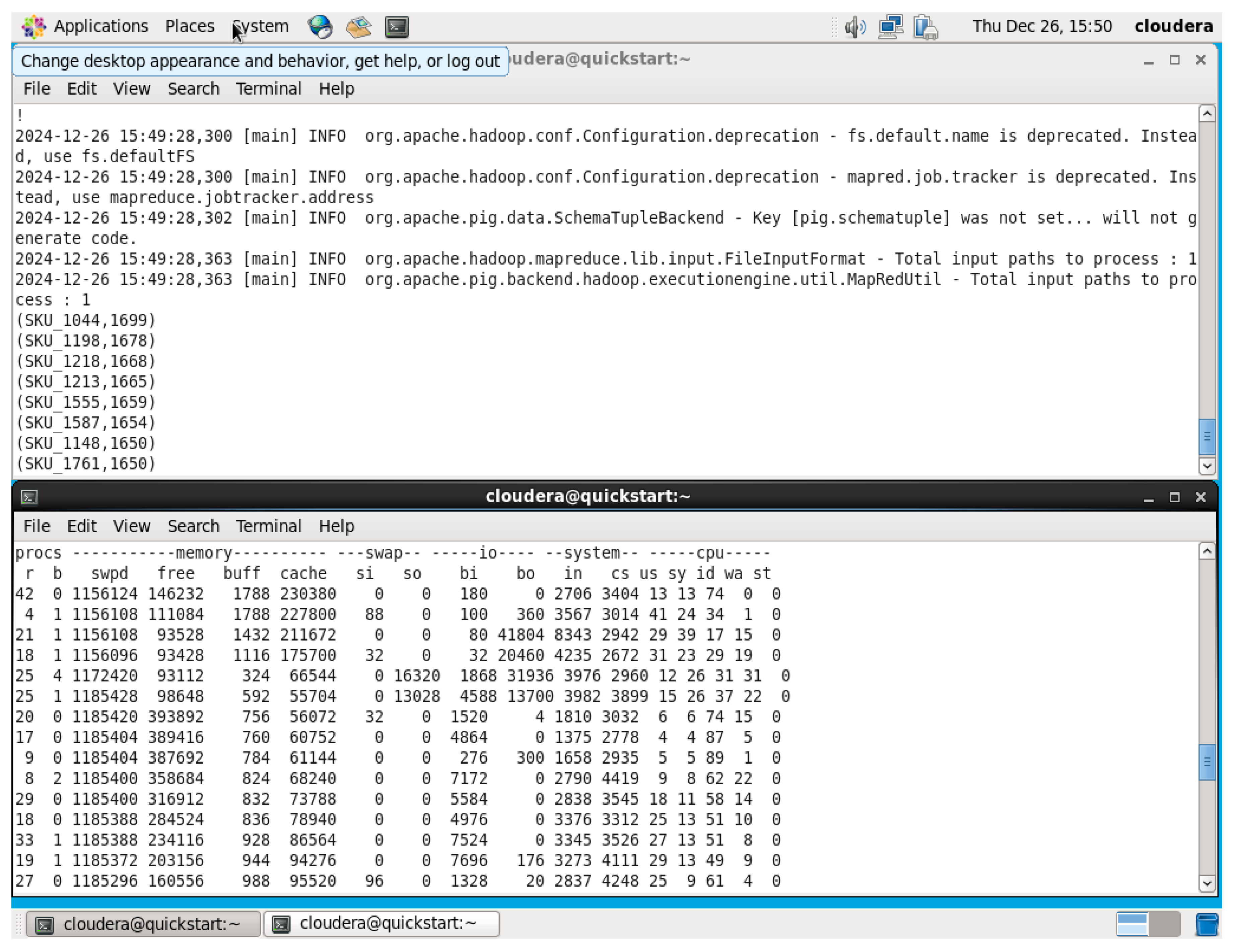
This query increased memory utilization drastically during its execution, where minimum free memory was 93,112.When the execution of queries was over and the terminal was closed, free memory reached again its maximum value, equal to 39,3832 KB, hence resources were well freed. This fluctuation in virtual memory utilization indicates the memory demands of the system during intensive data operations and the need for effective resource management when running large-scale queries in Pig. After it finished execution, it went back to 871,516kb.

6. Performance Comparison

A comparison between the three tools Hive, Impala and Pig is done based on three metrics: time taken to finish executing a query, virtual memory utilized while executing a query and the scalability.

Time Taken

	Hive	Impala	Pig
Time Taken in seconds (s)	39.911s	0.25s	199.60s

Figure 46. Execution time illustration.

Figure 46. Execution time illustration.

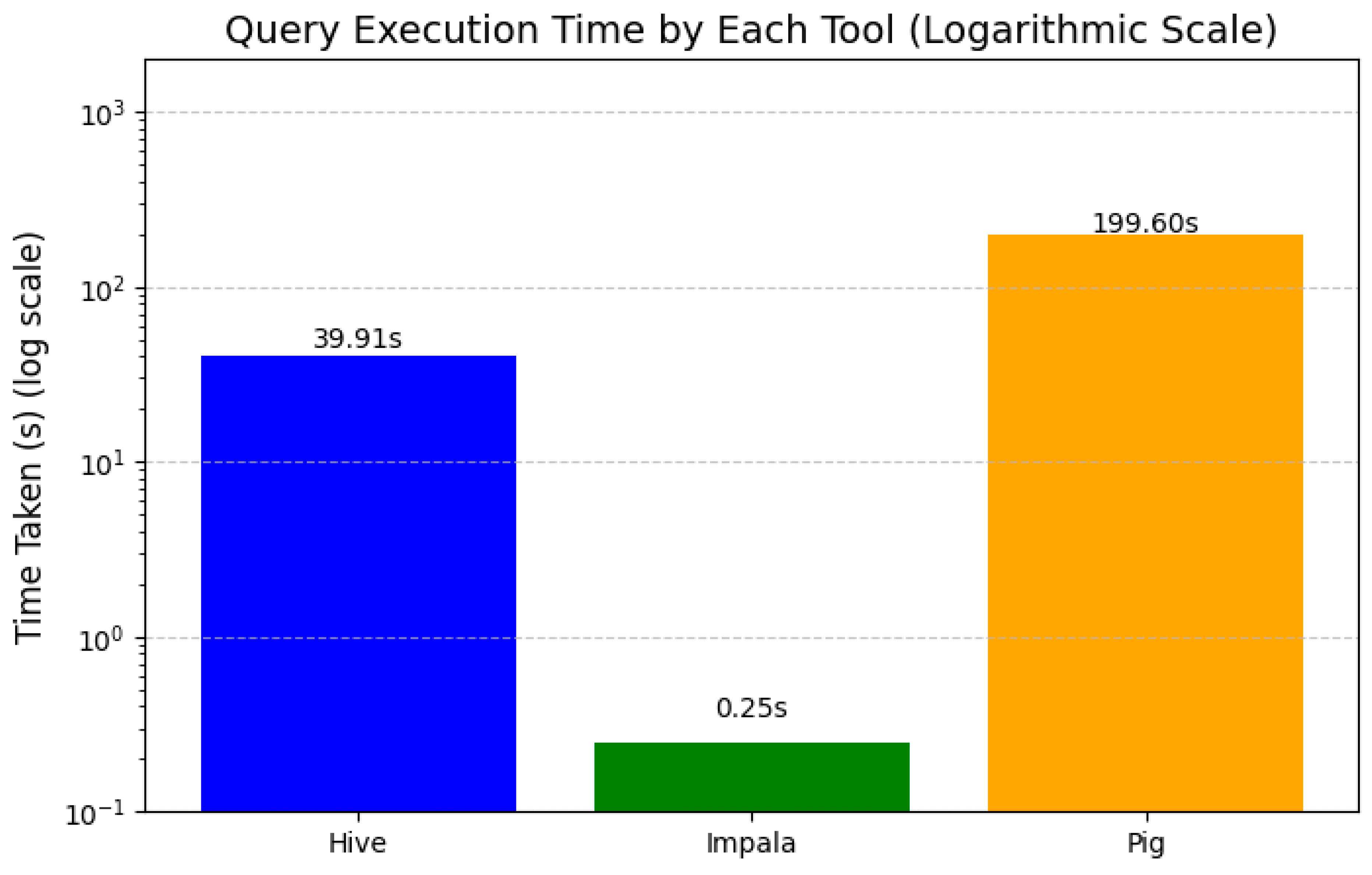
The execution time of the SQL-like query varies widely amongst the three big data tools: Hive, Impala, and Pig. Indeed, Pig has the highest execution time, with about 199.6 seconds, to emerge as the slowest. Hive performed moderately at roughly 39.91 seconds, while Impala recorded the fastest time with an execution time of just about 0.25 seconds.

This huge difference in execution times points to the performance characteristics of each tool. Impala is faster because of its in-memory processing engine, which avoids disk I/O overheads and gives very low latency. In contrast, Pig depends on batch processing through MapReduce, involving high disk operations and storage of intermediate data, hence the slow performance. Hive, though faster than Pig, is also based on a MapReduce-like execution model but applies additional query execution optimizations, hence its intermediary performance.

Results prove that for real-time or low latency analytics, Impala is suitable, whereas Hive and Pig are good candidates for batch-oriented processing, where the speed is not so important

Virtual Memory Utilization

	Hive	Impala	Pig
Free Memory Available (kb)	97,588 kb	461,418 kb	88,180 kb

Figure 47. Free Memory Available while execution illustration.

Figure 47. Free Memory Available while execution illustration.

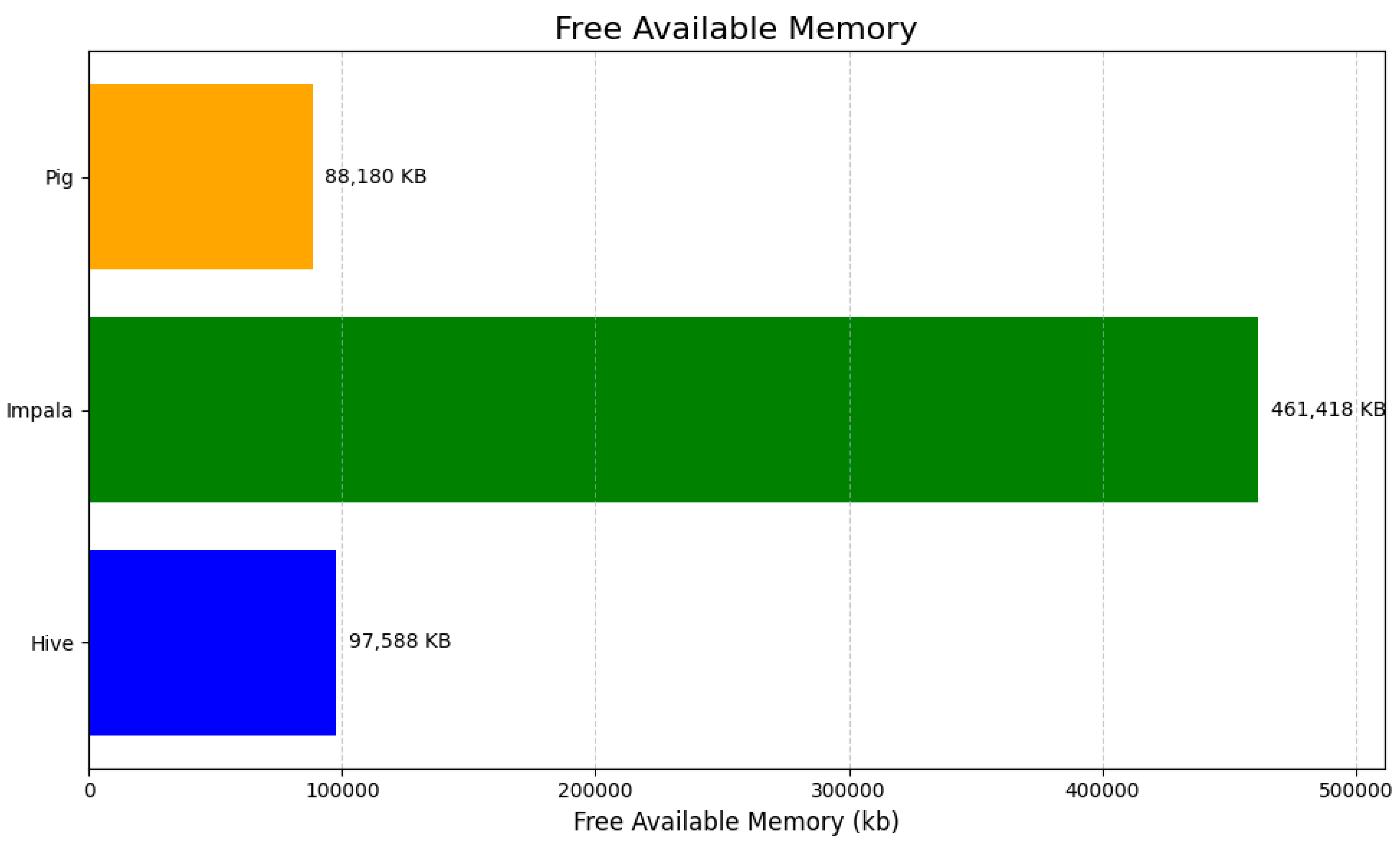
The horizontal bar chart visualizes the free available memory utilized by three big data tools—Hive, Impala, and Pig—measured in kilobytes (KB). Impala shows the highest memory utilization at 461,418 KB, significantly exceeding that of Hive (97,588 KB) and Pig (88,180 KB). The differences in memory usage highlight Impala’s more resource-intensive operations compared to the relatively lower memory demands of Hive and Pig. The chart effectively uses annotations to display exact memory usage for each tool, providing a clear and concise comparison.

Scalability

• Time Taken

	Hive	Impala	Pig
Time Taken in seconds (s)	43.324s	0.34s	181.32s

Figure 48. Query execution time comparison.

Figure 48. Query execution time comparison.

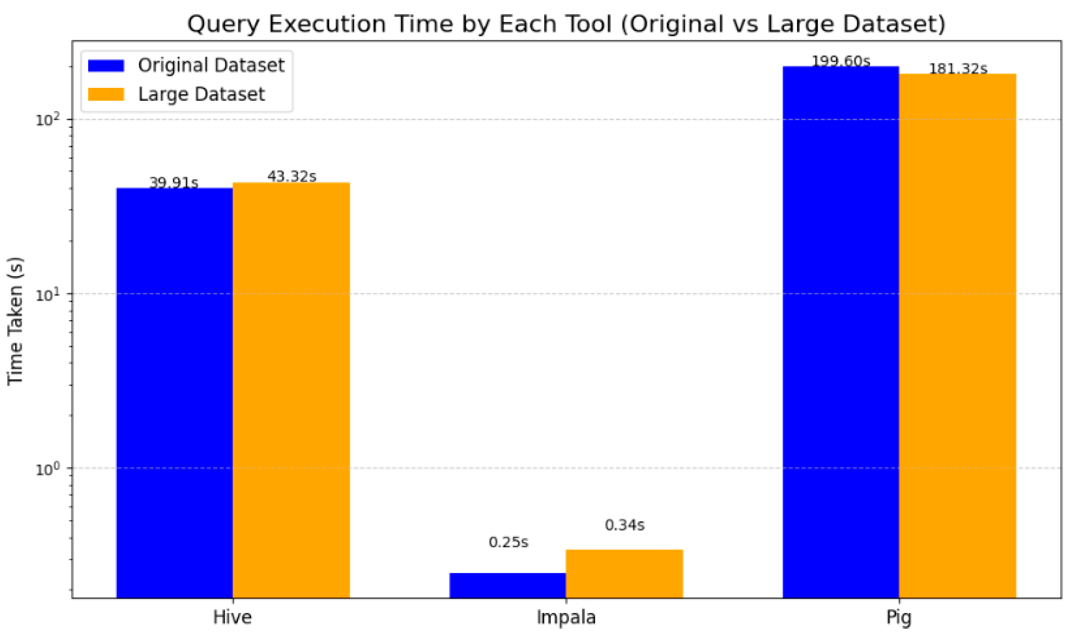
The bar chart illustrates the query execution times for three big data tools—Hive, Impala, and Pig—when applied to two datasets: the original dataset and a larger dataset. The y-axis is scaled logarithmically to effectively capture the significant variations in execution times across the tools. Hive exhibits a slight increase in execution time, rising from 39.91 seconds for the original dataset to 43.32 seconds for the larger dataset. Impala, known for its low-latency query performance, maintains exceptionally short execution times, increasing marginally from 0.25 seconds to 0.34 seconds as the dataset size grows. Interestingly, Pig demonstrates an improvement in execution efficiency for the larger dataset, with its execution time decreasing from 199.60 seconds to 181.32 seconds.

This comparison underscores the consistent efficiency of Impala, particularly for rapid query execution, while Hive and Pig reveal more variable performance patterns depending on dataset size and complexity.

• Virtual Memory Utilization

	Hive	Impala	Pig
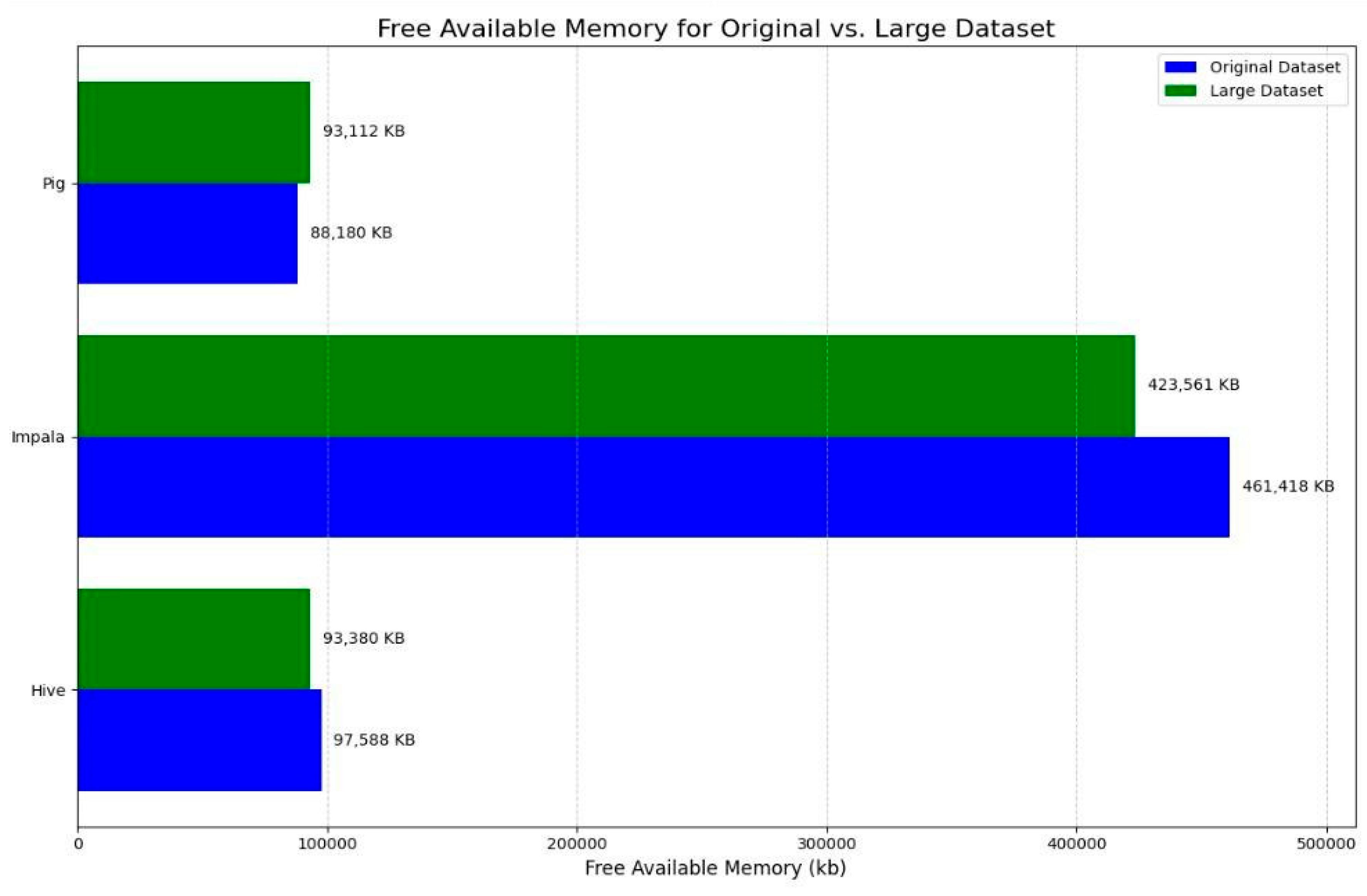
Virtual Memory Utilized (kb)	93,380 kb	423,561 kb	93,112 kb

Figure 49. Free Available Memory Comparison.

Figure 49. Free Available Memory Comparison.

7. Performance Visualization

Query results, discussion, and visualizations

1.

Executing 5 Queries on Hive

1st Query

Figure 50. Total Revenue by Country QUERY.

Figure 50. Total Revenue by Country QUERY.

Figure 51. Total Revenue by Country OUTPUT.

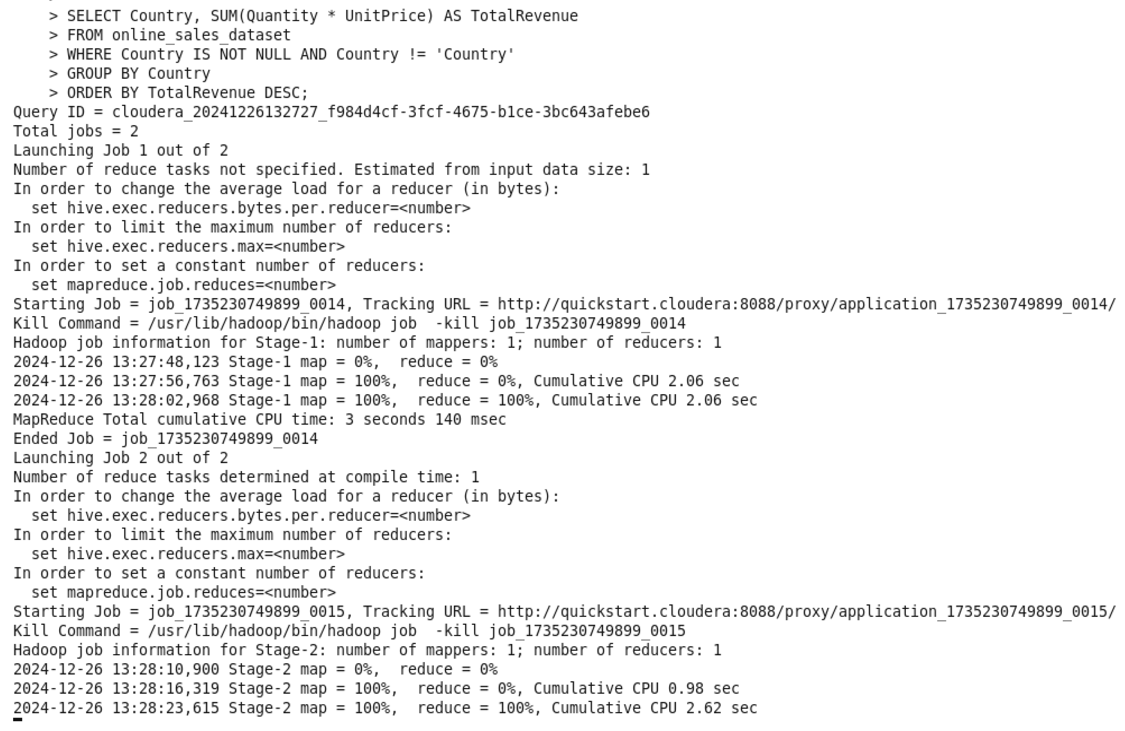
Figure 51. Total Revenue by Country OUTPUT.

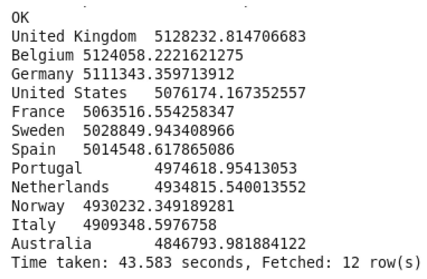
In the query command, it sums up transaction revenues as “TotalRevenues” by do a multiplication between “(Quantity * UnitPrice)” and grouping them by country to determine the total revenue earned per country. A condition was added to prevent a NULL value in front of

Country “WHERE Country IS NOT NULL AND Country != ‘Country’”. The top-performing countries are identified by sorting the output in order from highest country’s total revenue to lowest country. The insights driven from this query is to guide price plans, specific advertising efforts, and distribution of resources.

Figure 52. Total revenue by countries bar chart.

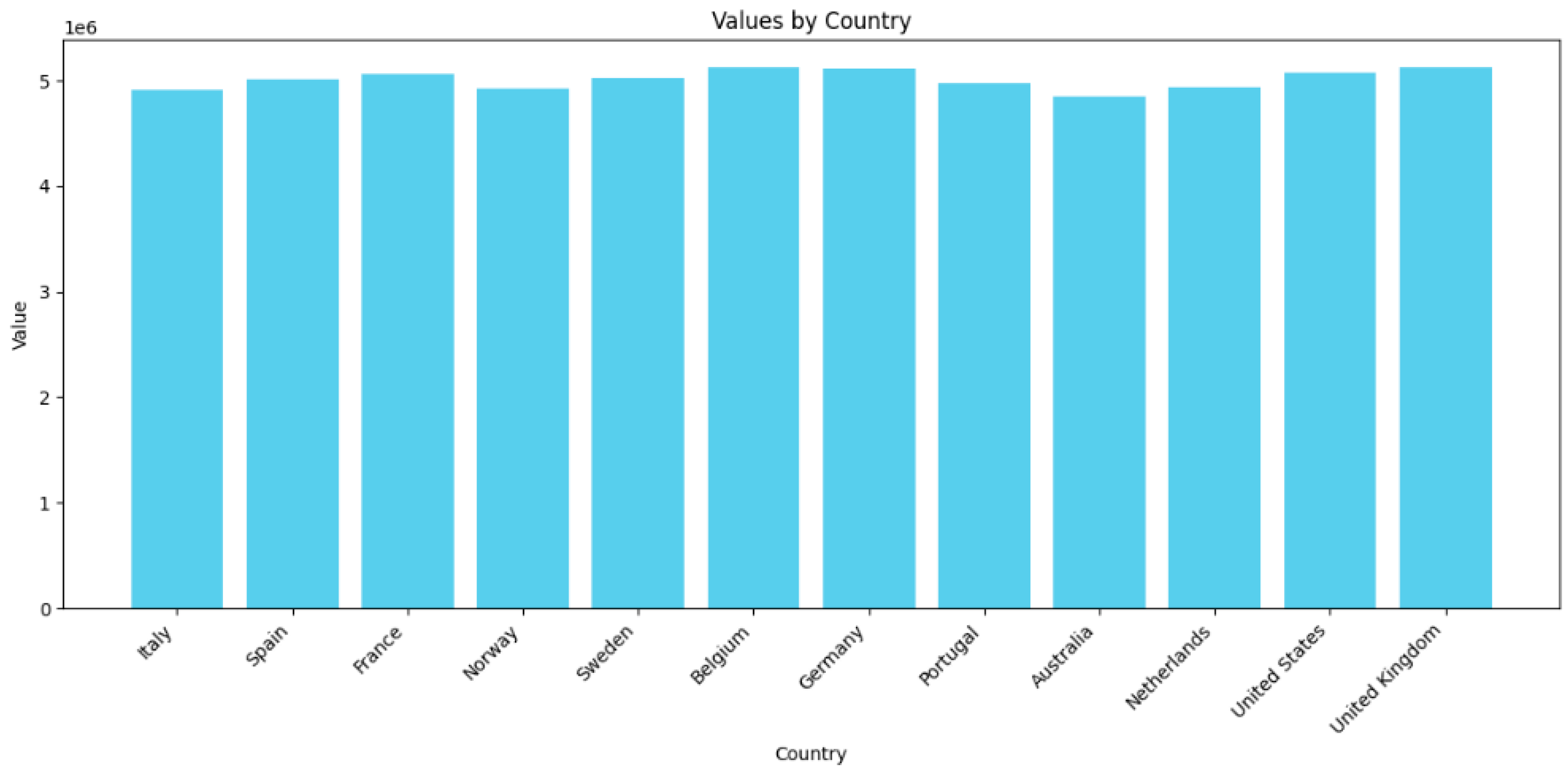
Figure 52. Total revenue by countries bar chart.

2nd Query

Figure 53. Top 10 Products by Quantity Sold QUERY.

Figure 53. Top 10 Products by Quantity Sold QUERY.

Figure 54. Top 10 Products by Quantity Sold OUTPUT.

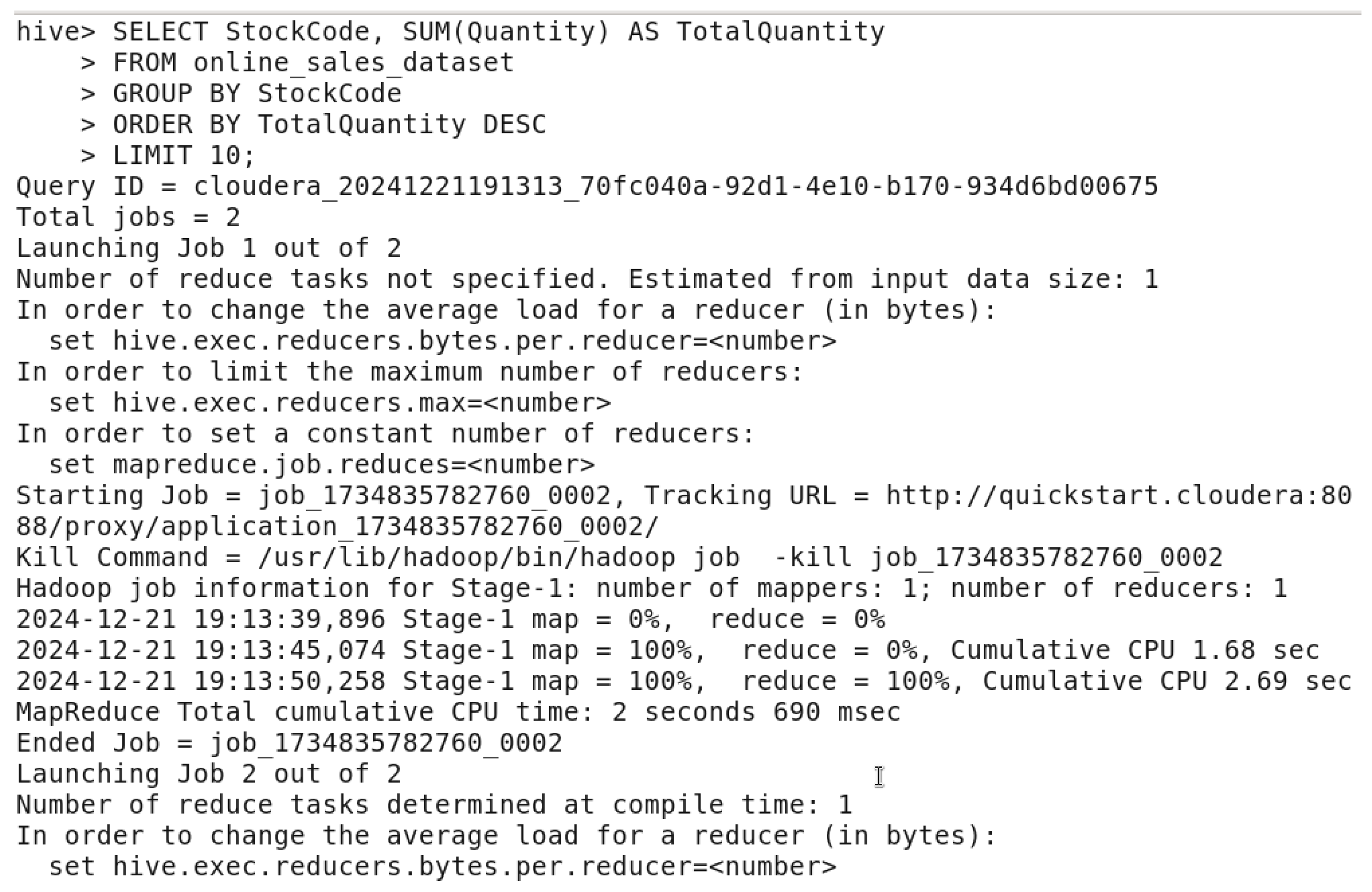
Figure 54. Top 10 Products by Quantity Sold OUTPUT.

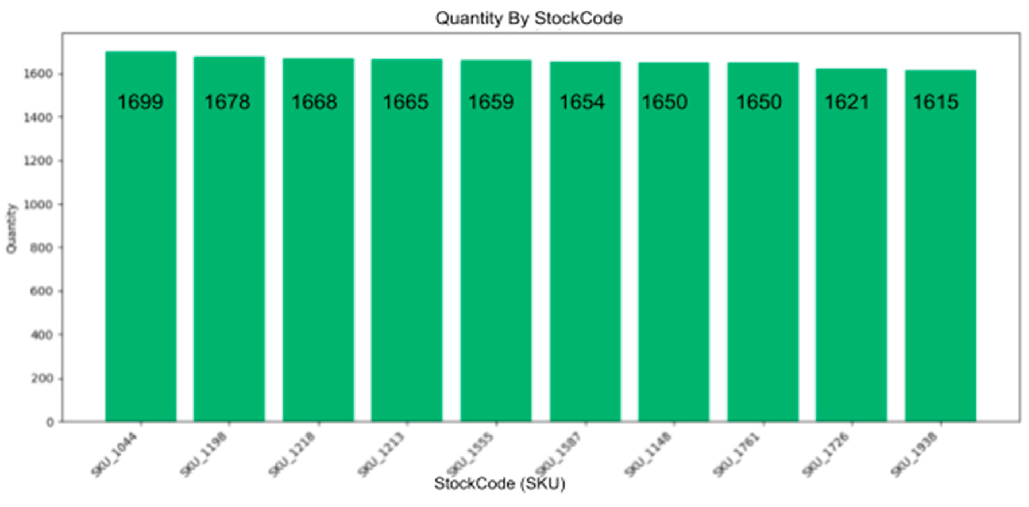
In the query command, it identifies the top 10 sold products by their quantity. Both “StockCode” and “Description” are grouped to calculate the “TotalQuantity” of the sold products using “SUM(Quantity)”, and sort the results from highest to highest sold ones to the lowest sold ones. This query reveals the most desirable products, allowing companies to set priorities for inventory management, enhance marketing strategies, and concentrate on those that bring the highest revenue.

Figure 55. Top 10 products by quantity sold bar chart.

Figure 55. Top 10 products by quantity sold bar chart.

3rd Query

Figure 56. Yearly Sales Query.

Figure 56. Yearly Sales Query.

Figure 57. Yearly Sales Query Output 1&2.

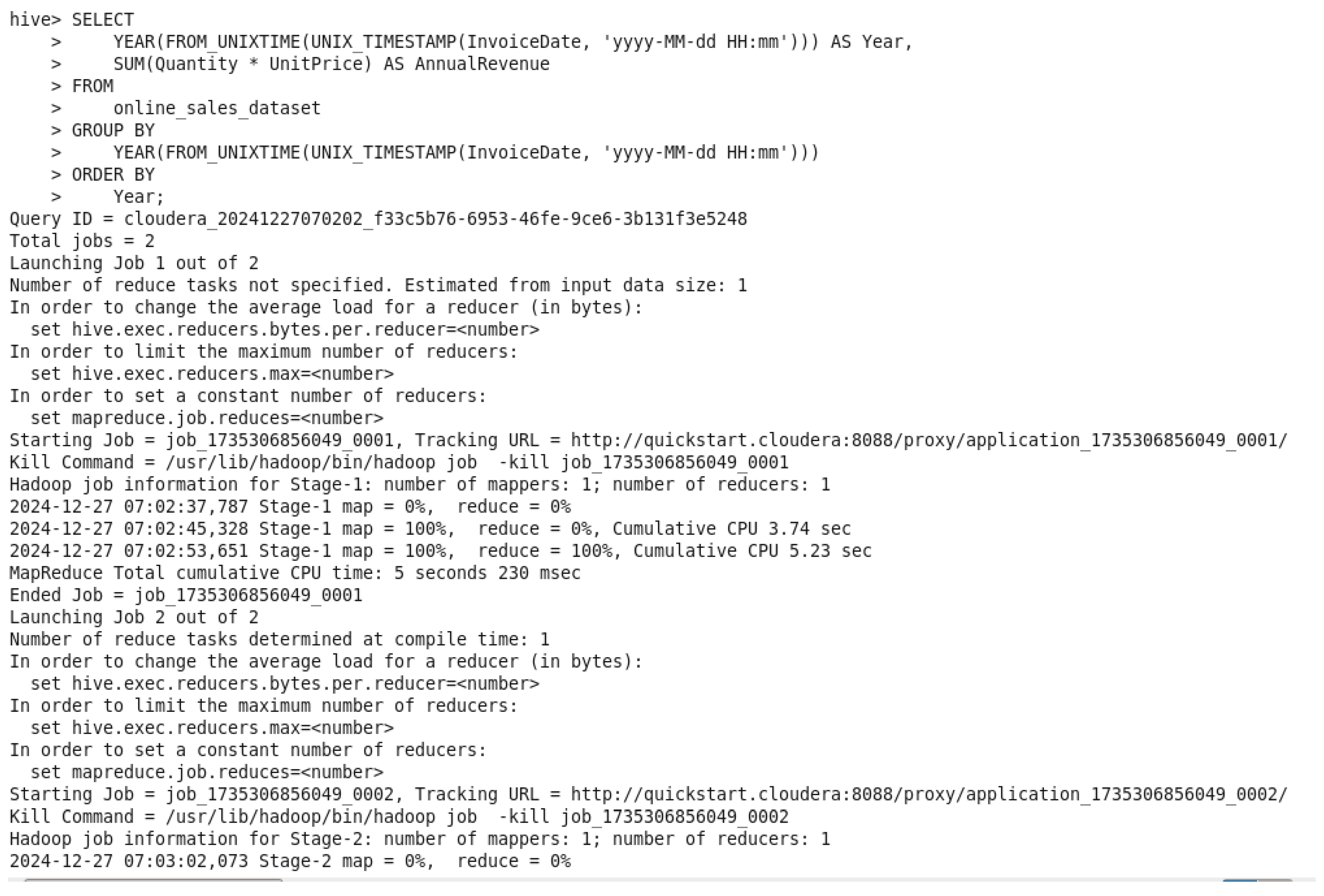
Figure 57. Yearly Sales Query Output 1&2.

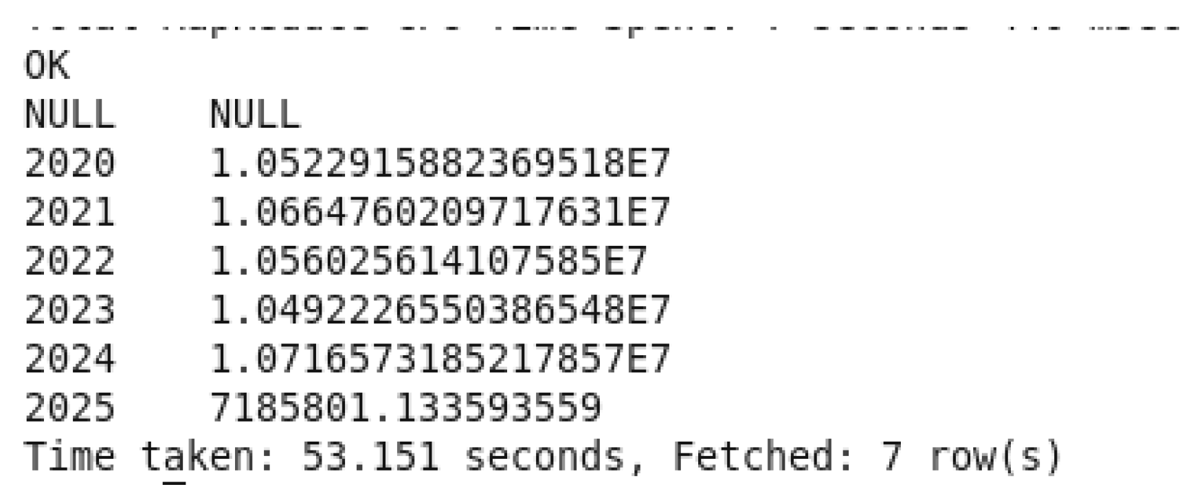
The previous query command was to calculate the total revenue each year by taking out the year from “InvoiceDate” and then sums up the revenue by a multiplication between (Quantity * UnitPrice” for every year. The results will be both sorted and grouped by the years. This is deriving insights about the overall sales trends over time, making it possible to assess the growth and performance of the company. Through the identification of revenue changes, companies are able to evaluate how plans and competition affect their annual results.

Figure 58. Yearly sales trends illustrations.

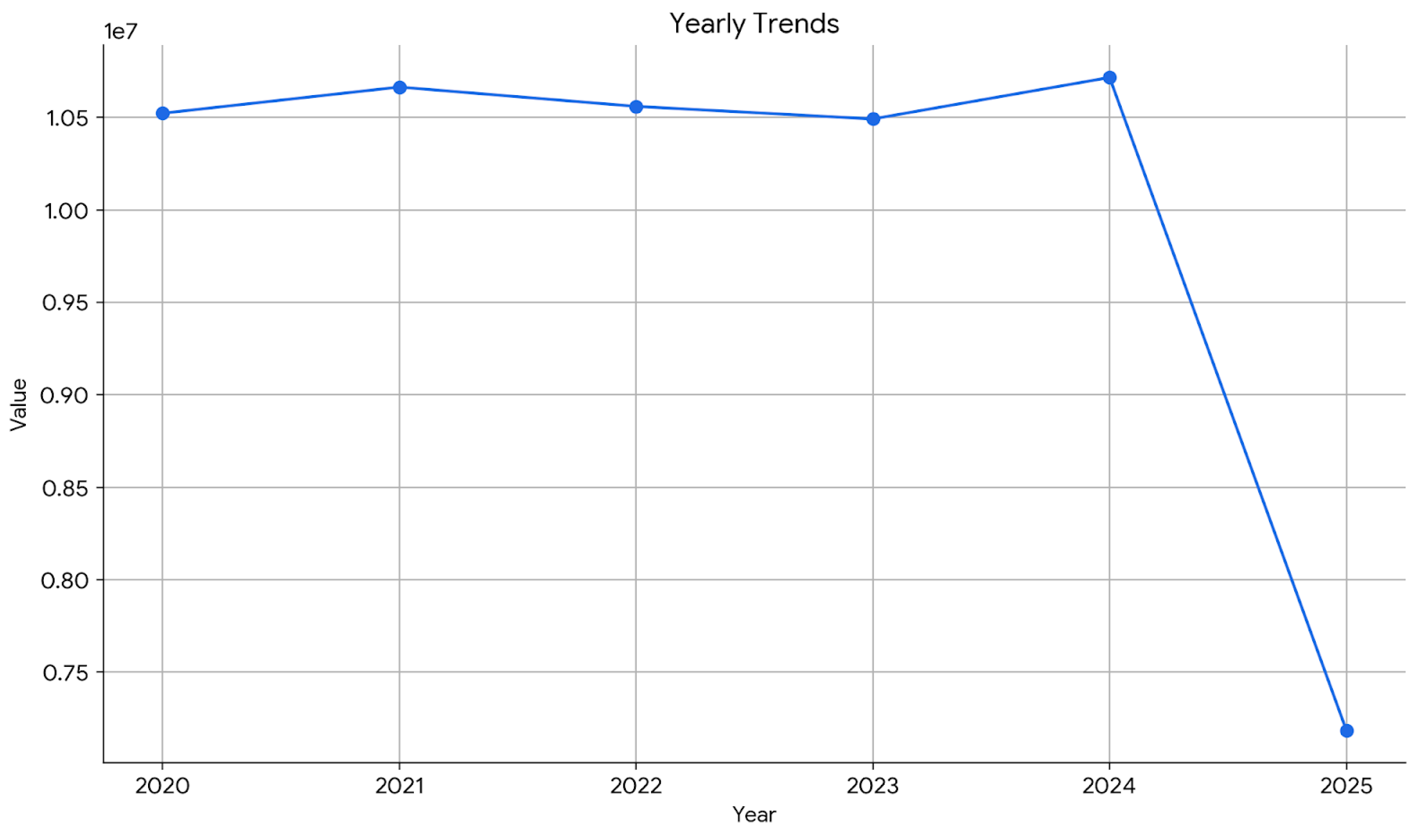
Figure 58. Yearly sales trends illustrations.

4th Query

Figure 59. Average Discount per Product Category Query.

Figure 59. Average Discount per Product Category Query.

Figure 60. Average Discount per Product Category Query Output.

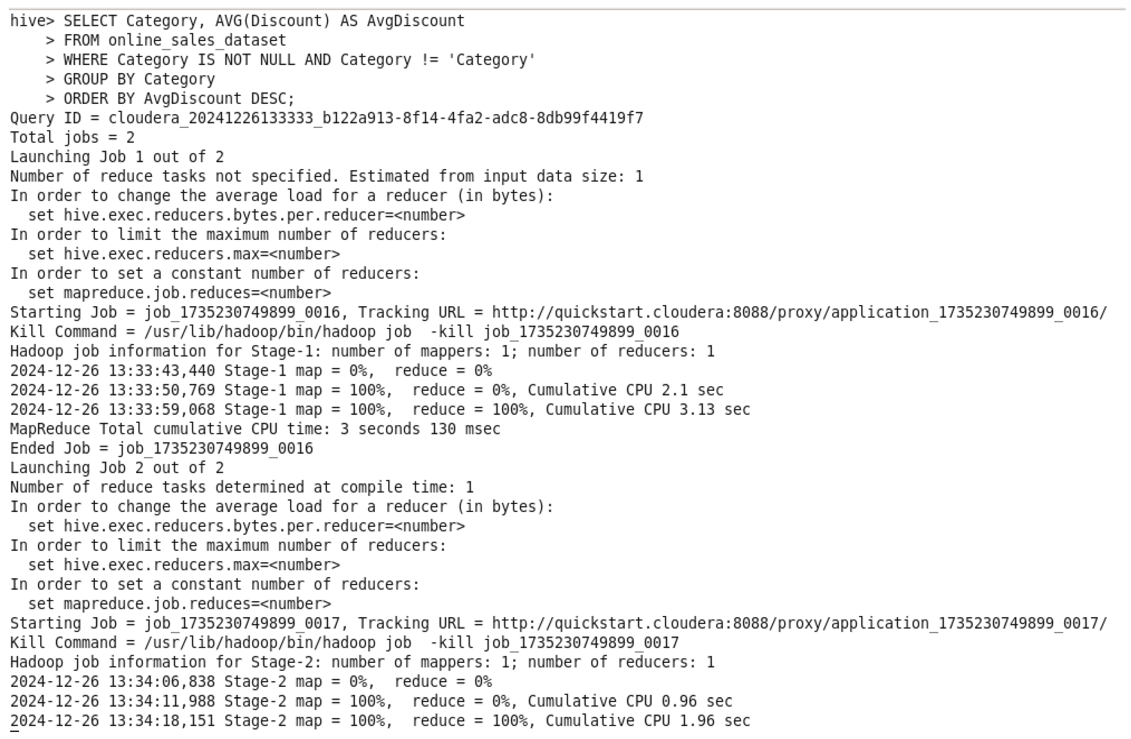
Figure 60. Average Discount per Product Category Query Output.

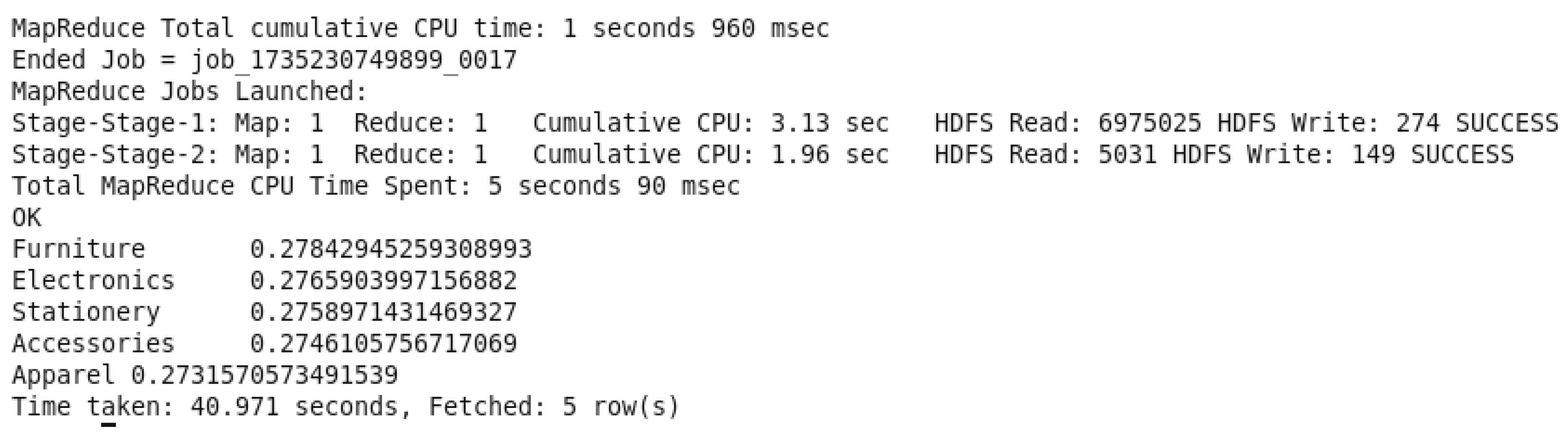
The command of the query is determining the average discount “AvgDiscount” for each category of the product by using “AVG(Discount)”. A condition was added to prevent a NULL value in front of Category “WHERE Category IS NOT NULL AND Category != ‘Category’”. It then classifies the data by the category, demonstrating the categories with the largest average discounts. Companies can use such data to enhance pricing, analyze the success of advertisements, and figure out how discounts affect sales and customer behavior.

Figure 61. Average Discount Per Product Category illustrations.

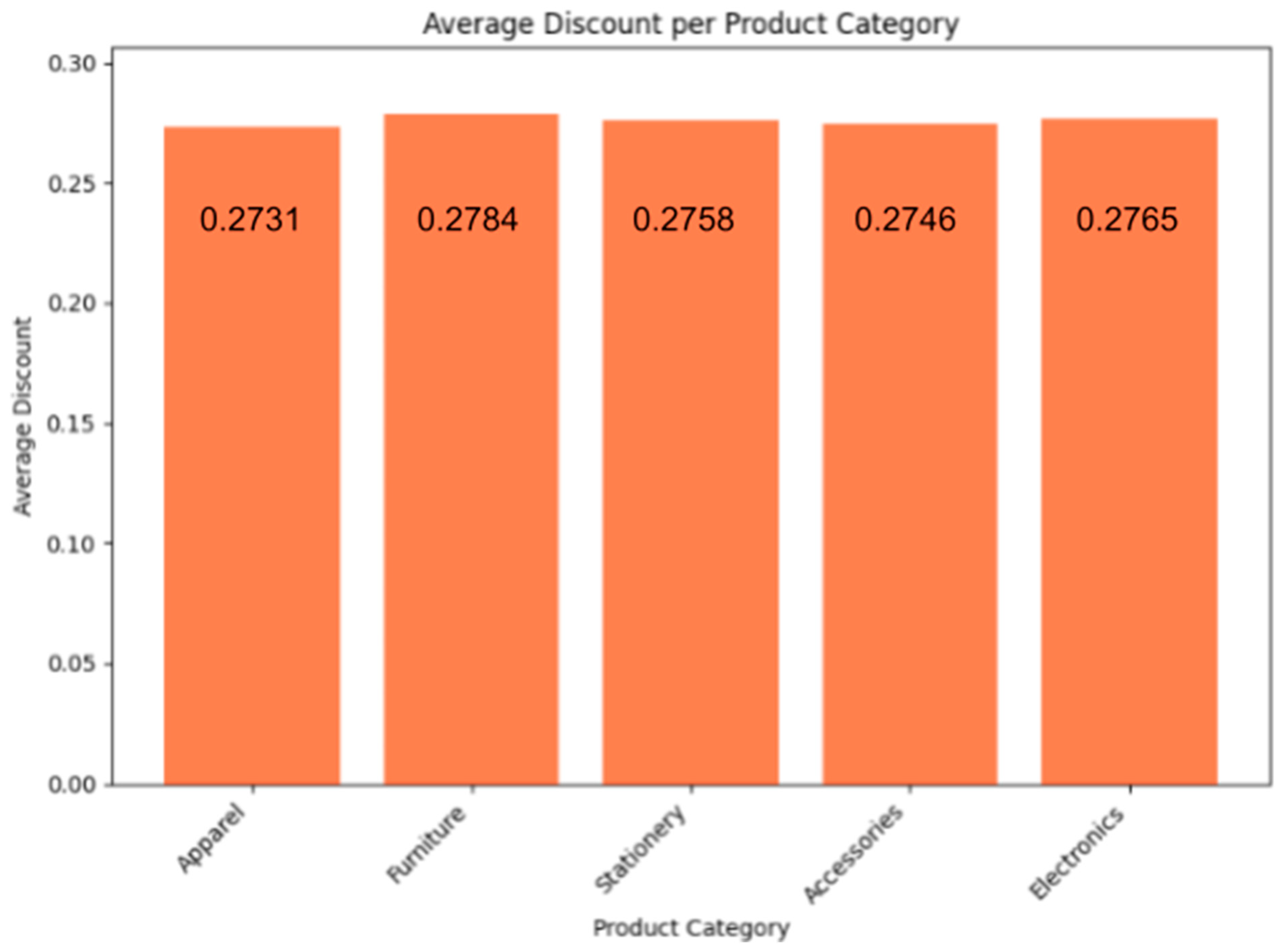
Figure 61. Average Discount Per Product Category illustrations.

5th Query

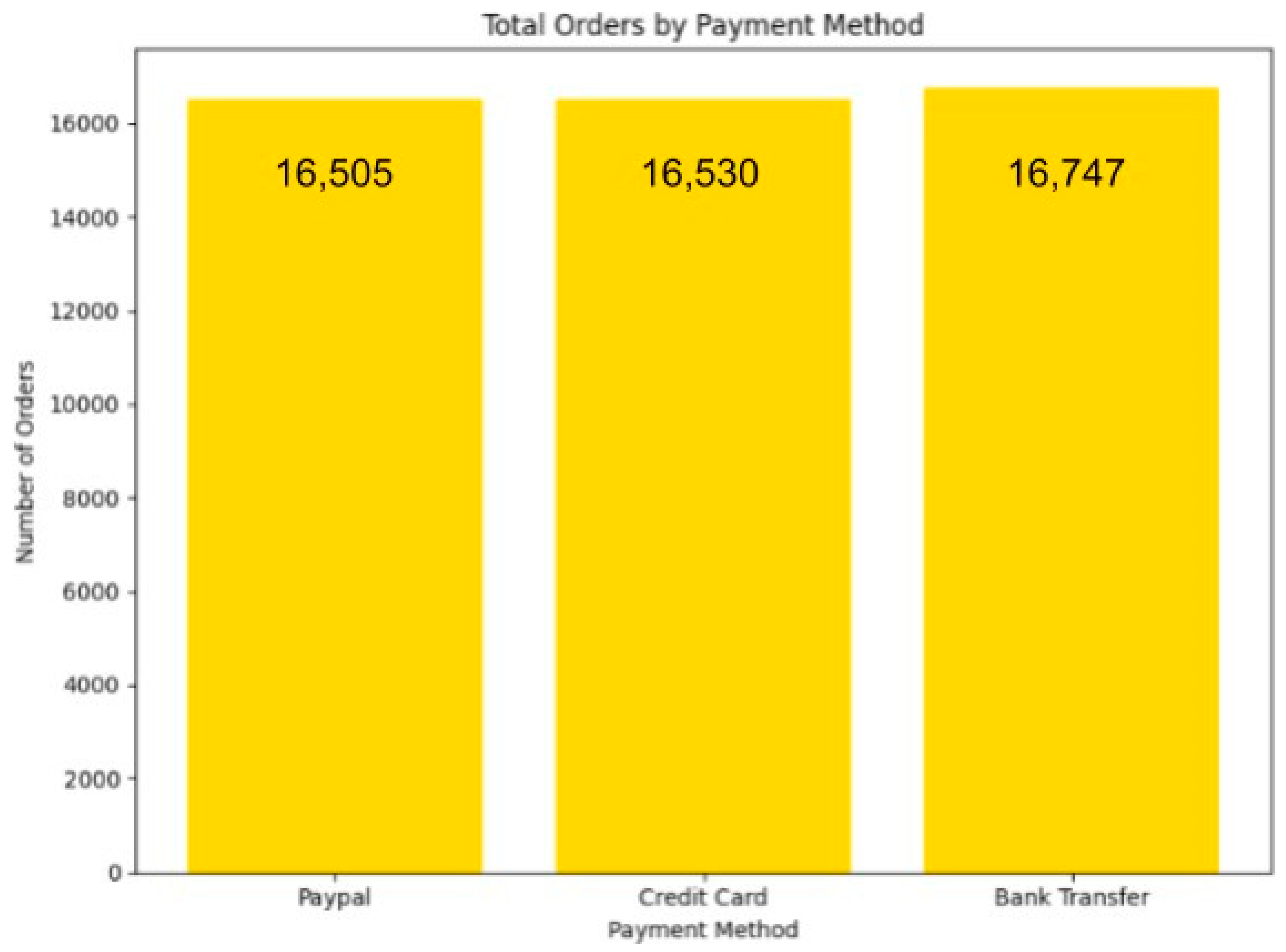
Figure 62. Total Orders by PaymentMethod Query.

Figure 62. Total Orders by PaymentMethod Query.

Figure 63. Total Orders by PaymentMethod QueryOutput.

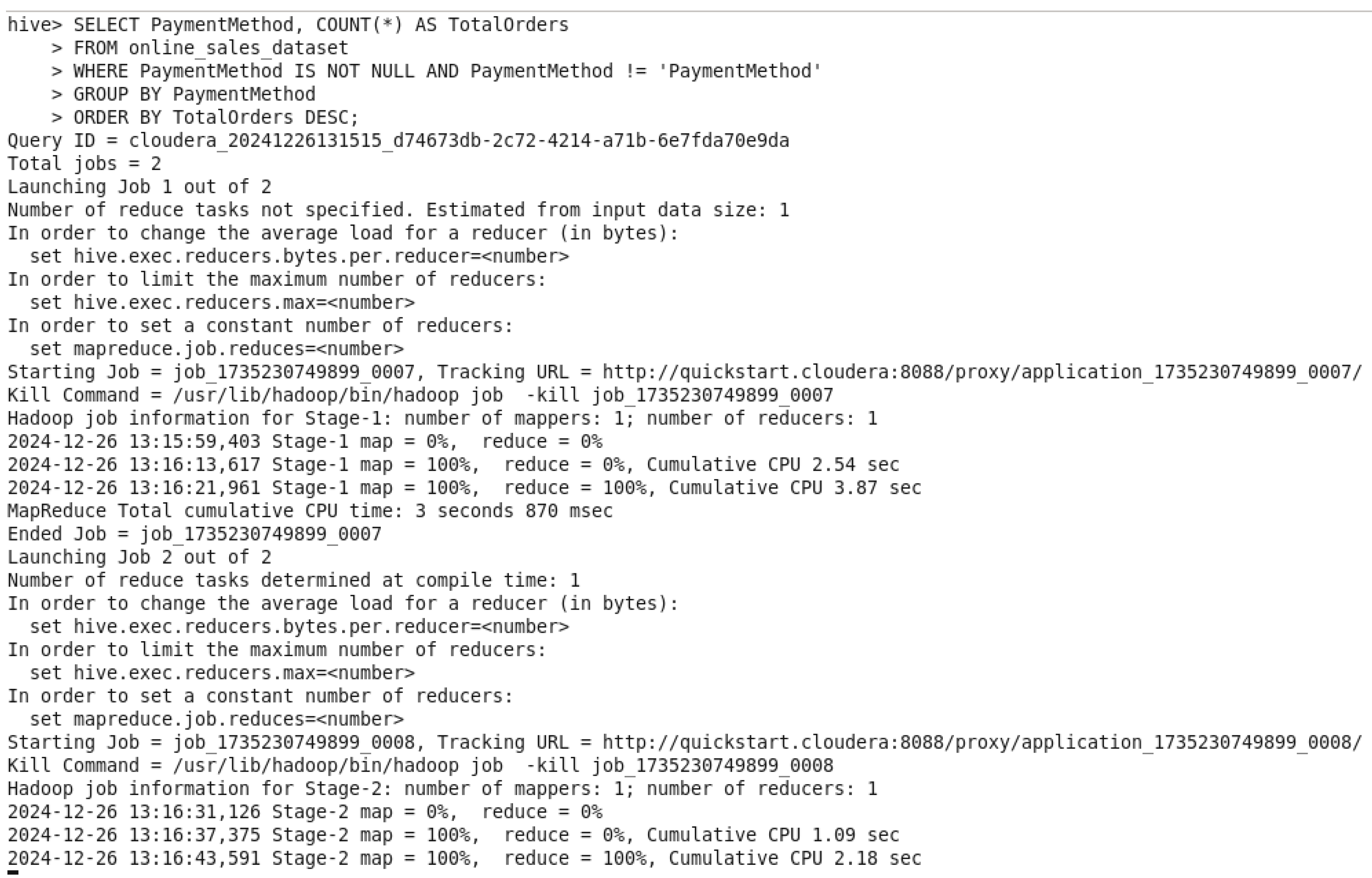
Figure 63. Total Orders by PaymentMethod QueryOutput.

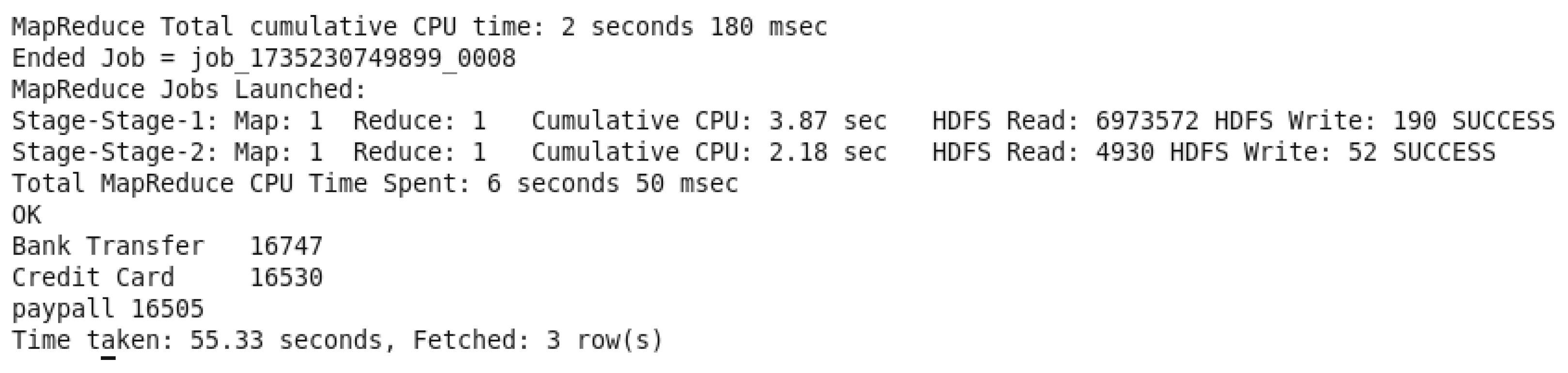
This query is grouping out the orders by “PaymentMethod” and sorting them from highest payment method number to lowest number, and that’s to determine the total number of orders in each payment method used. A condition was added to prevent a NULL value in front of PamentMethod “WHERE PamentMethod IS NOT NULL AND PamentMethod != ‘PamentMethod’”. This query is giving insights to reveal the most popular used payment options and then to give recommendations to add more options and to maximize client comfort, which will improve the overall payment experience.

Figure 64. Total Orders By Payment Methods illustration.

Figure 64. Total Orders By Payment Methods illustration.

1.

Executing 5 Queries on Pig

1st Query - Total Revenue by Country QUERY: This Pig query calculates the total revenue by country by multiplying quantity and unit price, then grouping by country.

Figure 65. Total Revenue by Country QUERY & OUTPUT.

Figure 65. Total Revenue by Country QUERY & OUTPUT.

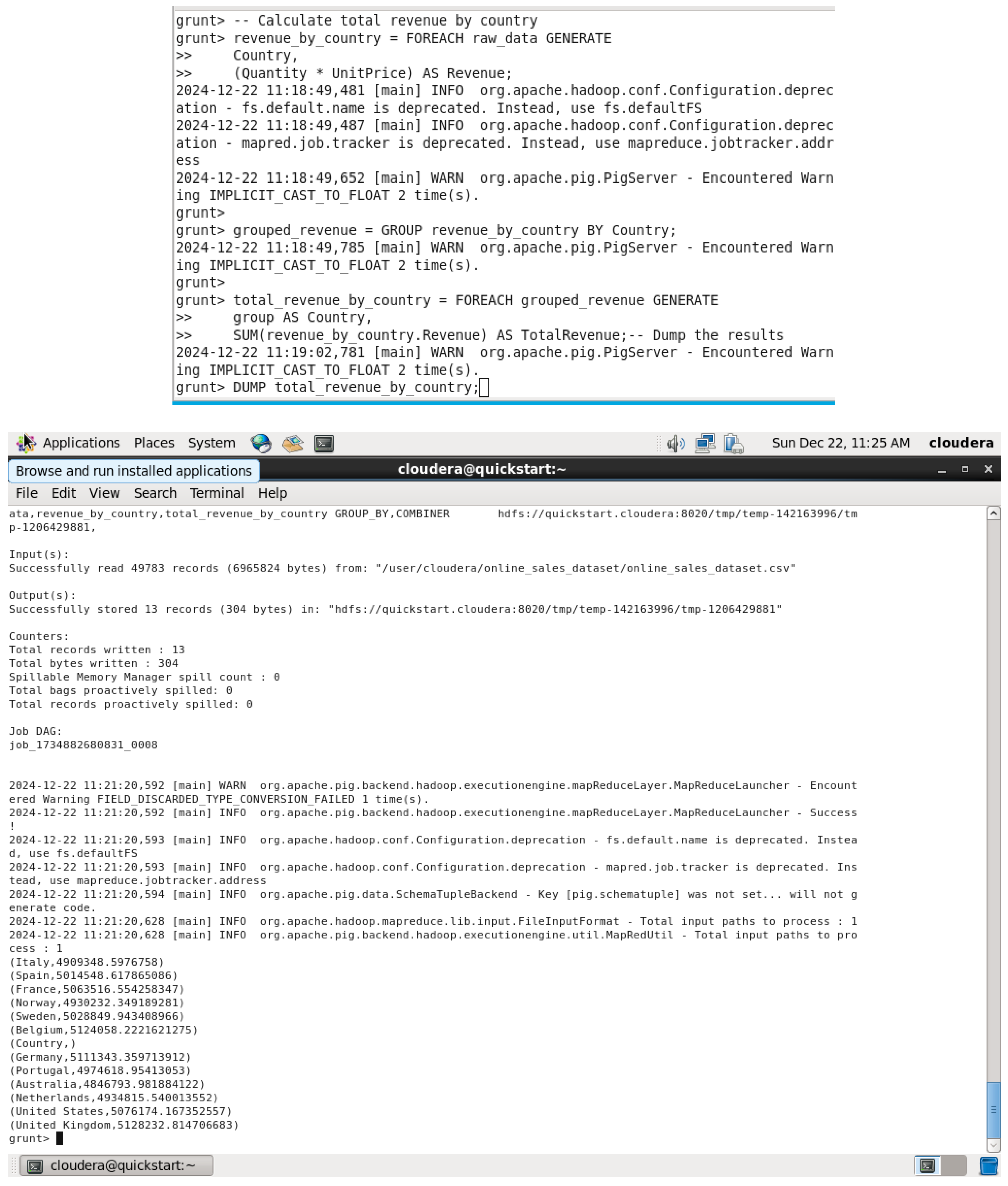
This query loads the dataset from a CSV file into the sales_data variable, declaring the data types for each field. It then groups the data by the country field to enable country-specific analysis. The FOREACH operation calculates the total revenue for each country by multiplying quantity and unit_price for each order, summing the results per group. Then it orders them in descending order of total_revenue and thus countries with a higher revenue will appear first. The results are finally dumped onto the screen via the DUMP command.

2nd Query - Top 10 Products by Quantity Sold QUERY: This query returns the top 10 products by quantity sold

Figure 66. Top 10 Products by Quantity Sold QUERY & OUTPUT.

Figure 66. Top 10 Products by Quantity Sold QUERY & OUTPUT.

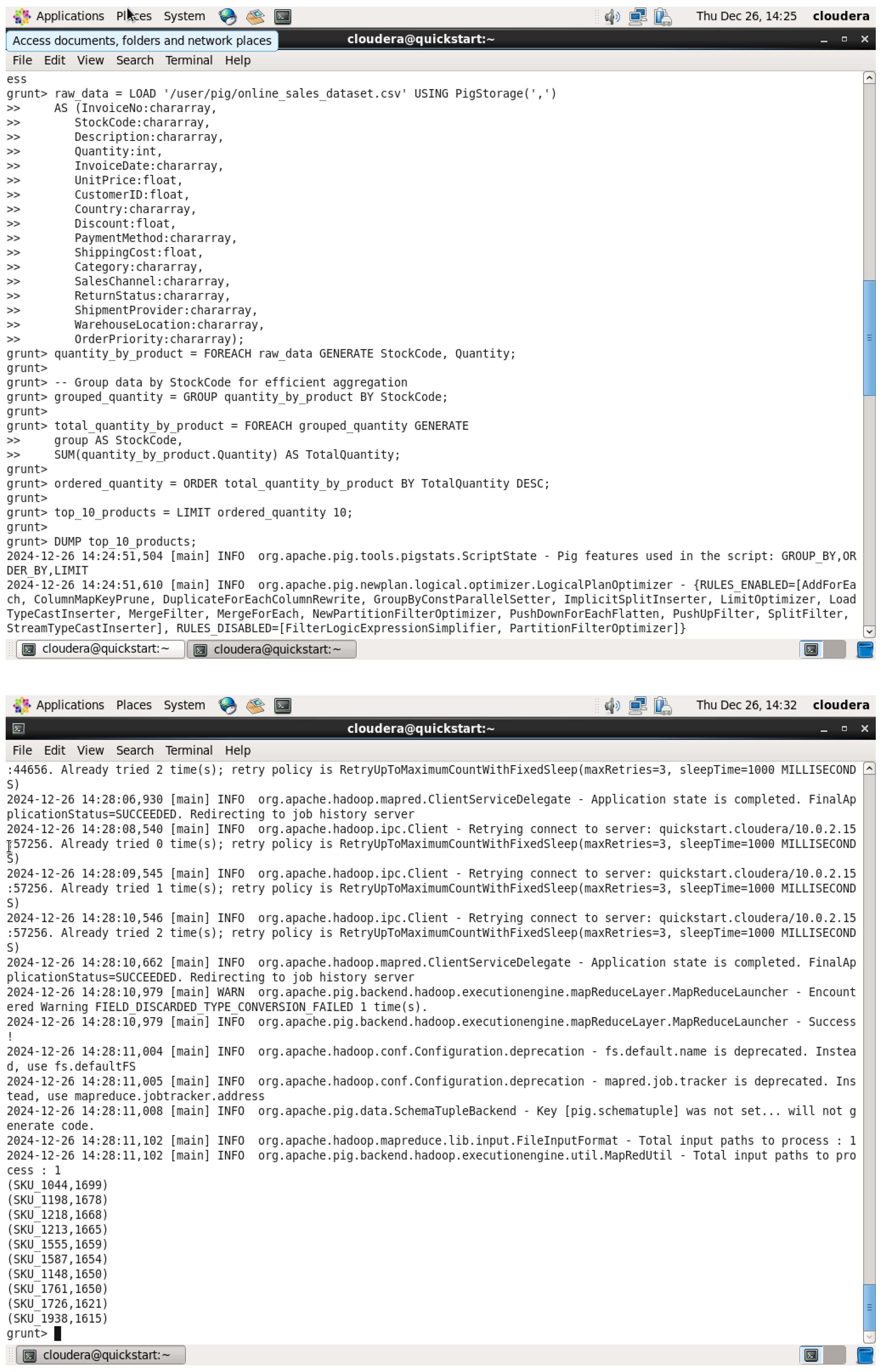
This query first loads the data into sales_data, groups it on the product_name field for aggregating the sales data product-wise, and uses the FOREACH command to sum up the quantity field of each product for finding the total quantity sold of each product. The results are sorted in descending order of the total quantity sold so that the most sold products are at the top. LIMIT only restricts the output of the top 10 products, whereas DUMP is a command to present the results of this limitation.

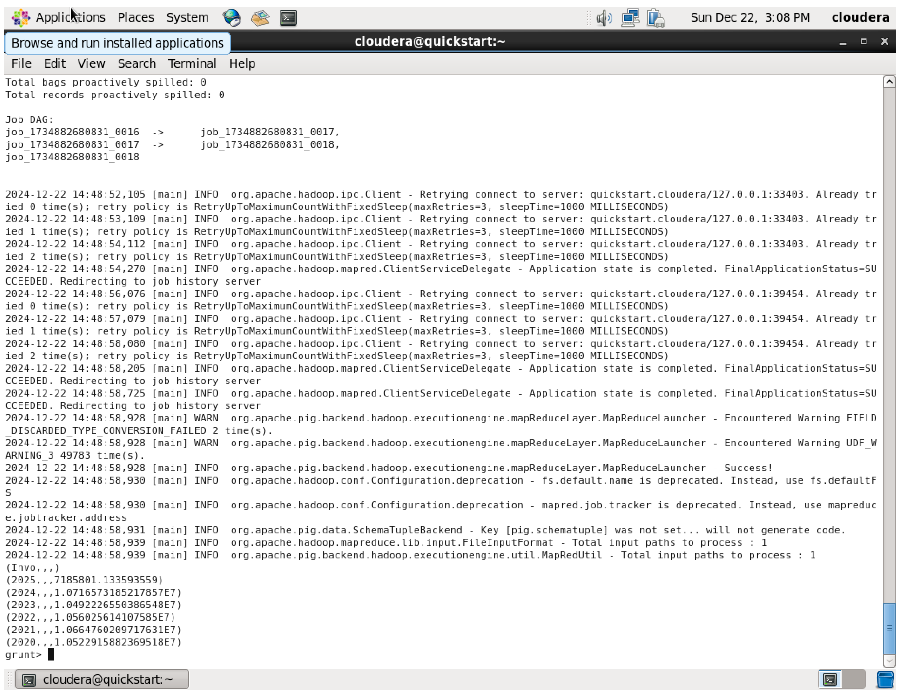
3rd Query

Figure 67. Yearly Sales QUERY Output.

Figure 67. Yearly Sales QUERY Output.

This query begins by loading in the dataset and then converts the string order_date to a date format with ToDate; YEAR and MONTH are used on the order_date, so now there can be analysis done monthly. This groups all of the data by both year and month, while Totals are calculated as quantity multiplied by unit_price for every month. Results ordered by year and month to display the sales trend in chronological order. Finally, the DUMP command is used to display the monthly sales trends.

4th Query

Figure 68. Average Discount per Product Category QUERY.

Figure 68. Average Discount per Product Category QUERY.

Figure 69. Average Discount per Product Category QUERY (continuous).

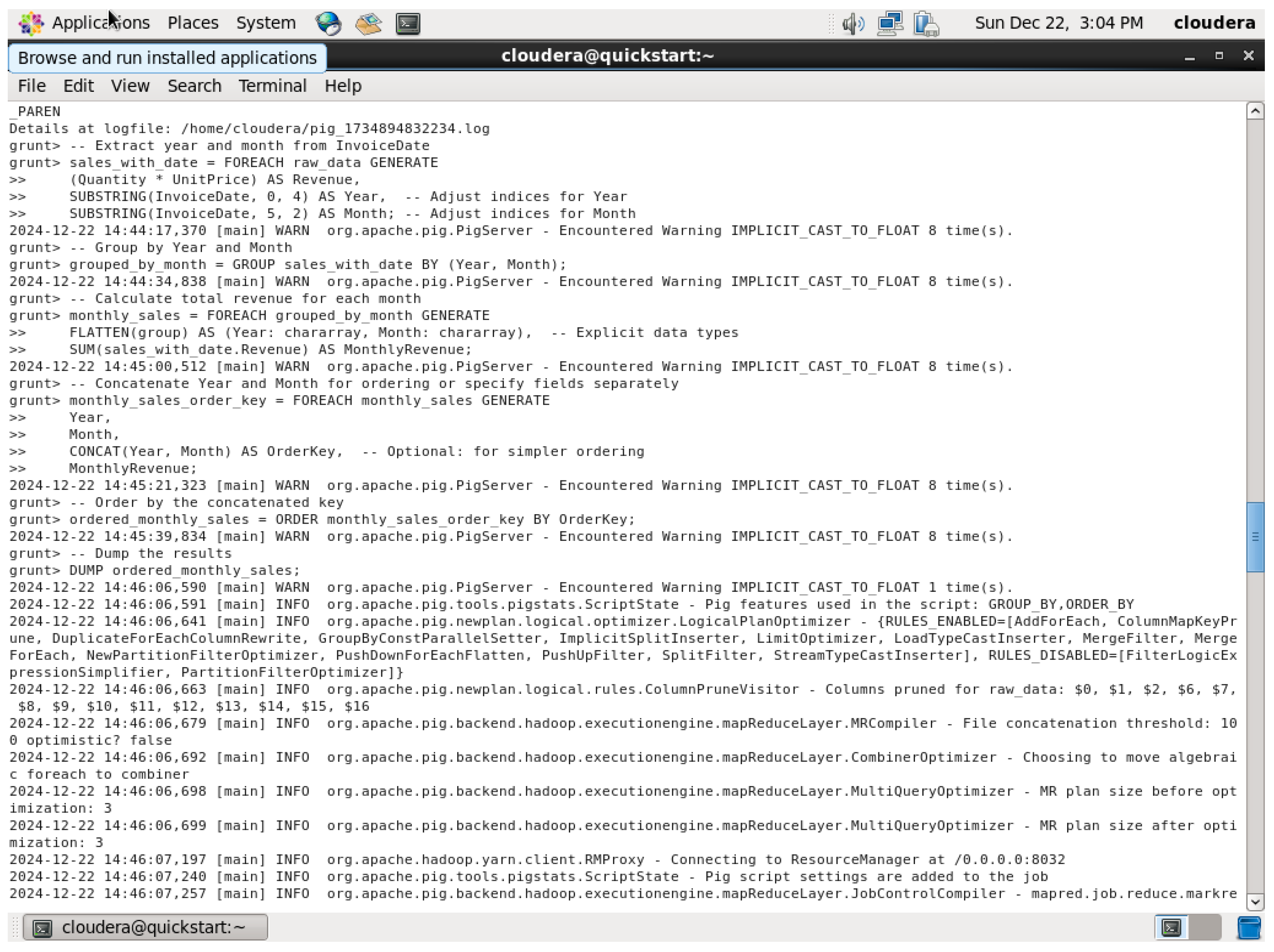
Figure 69. Average Discount per Product Category QUERY (continuous).

Figure 70. Average Discount per Product Category QUERY Output.

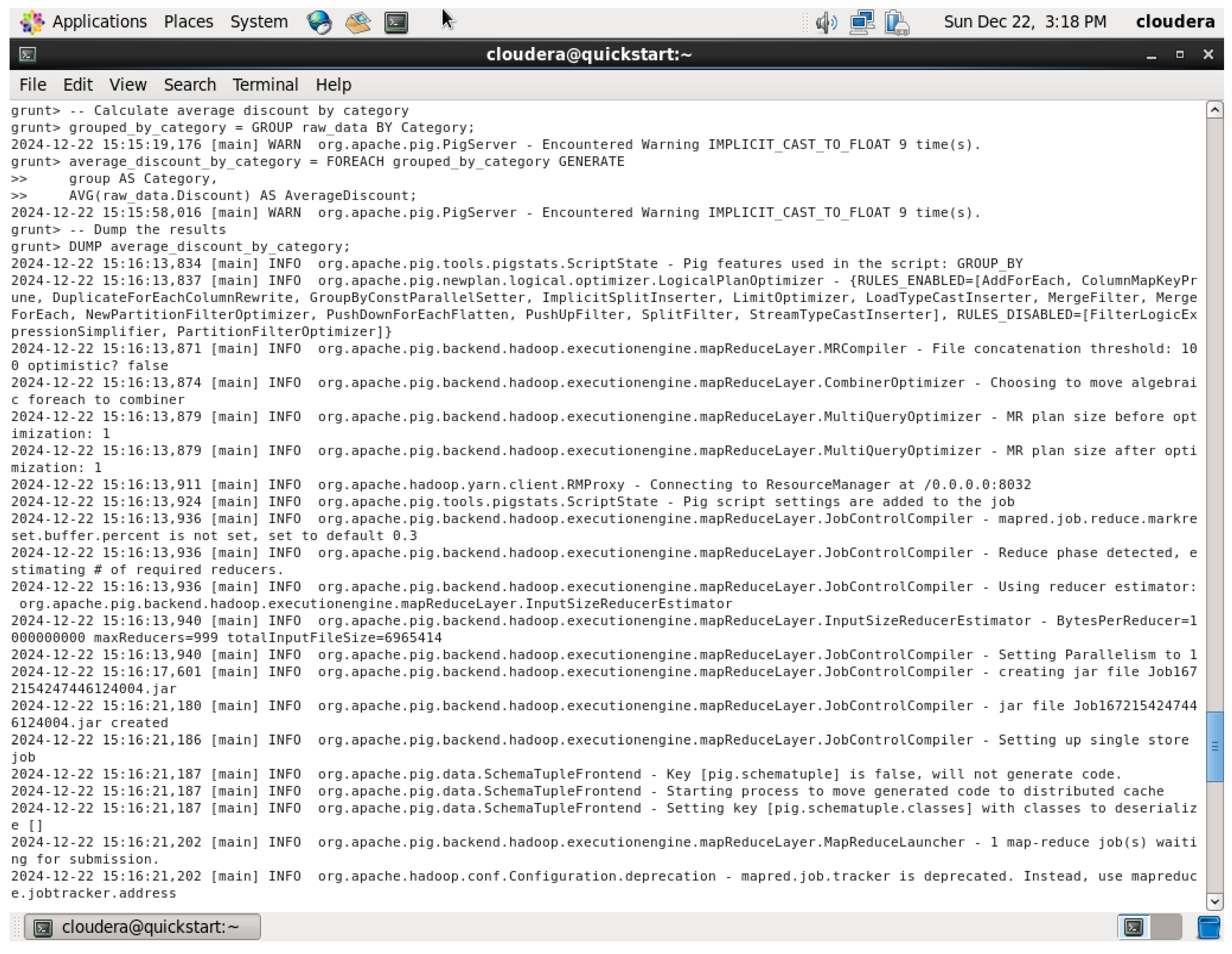
Figure 70. Average Discount per Product Category QUERY Output.

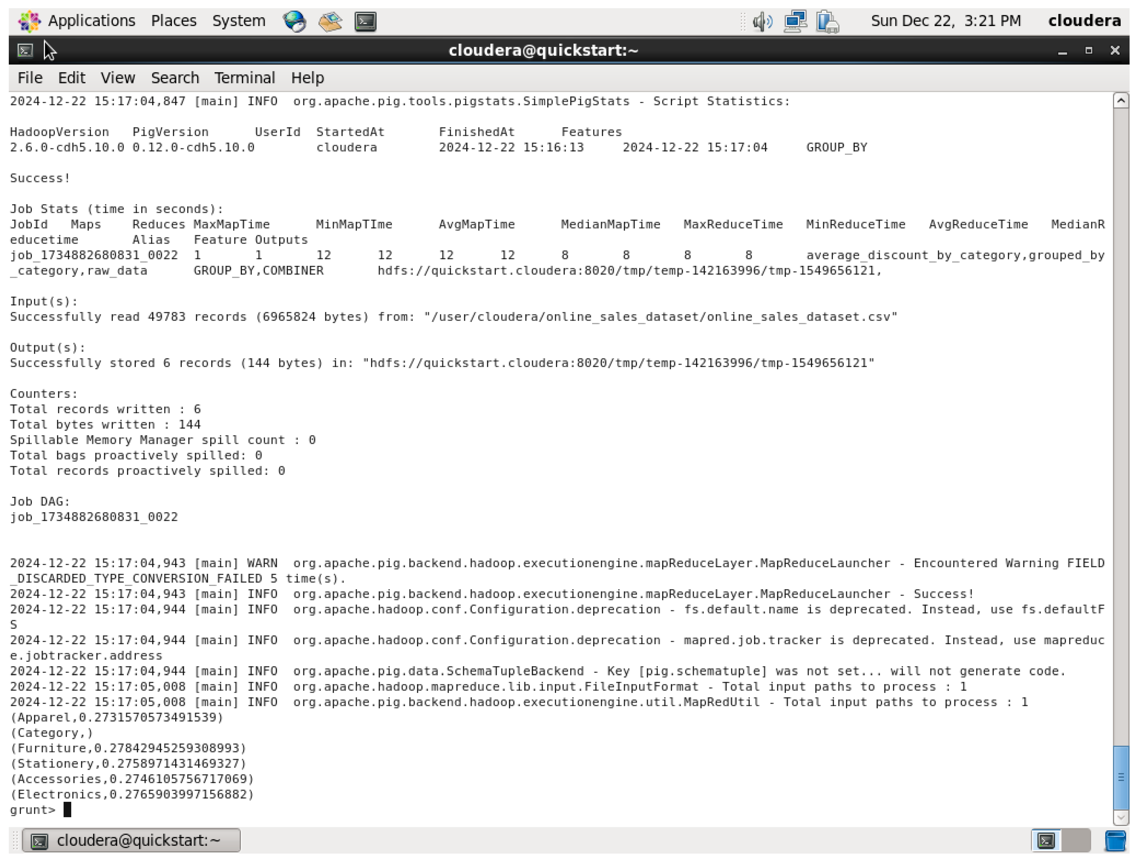
The dataset in the query above was loaded, then grouped by the product category to establish an average discount for each of those categories. Here, the AVG function is used on the discount field so that it returns the average of every product category’s discount. The DUMP command was used here to show the average of the discount in each category of the dataset.

5th Query This query calculates the total number of orders by payment method

Figure 71. Total Orders by PaymentMethod QUERY.

Figure 71. Total Orders by PaymentMethod QUERY.

Figure 72. Total Orders by PaymentMethod QUERY Output.

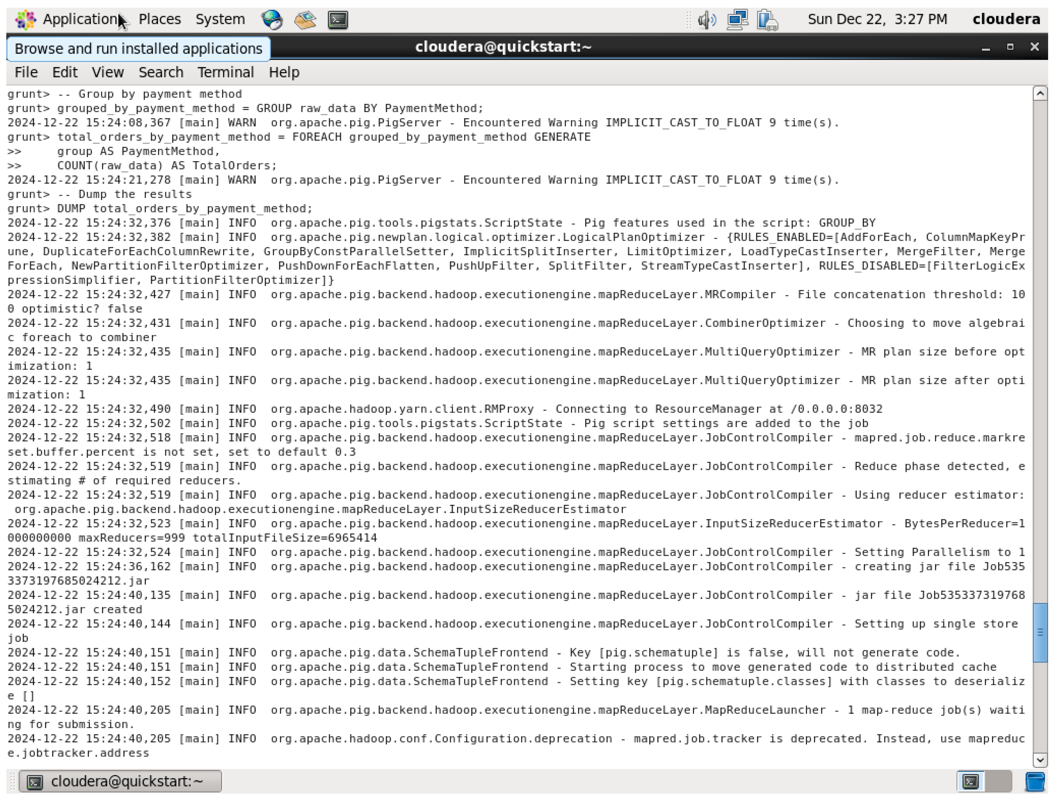
Figure 72. Total Orders by PaymentMethod QUERY Output.

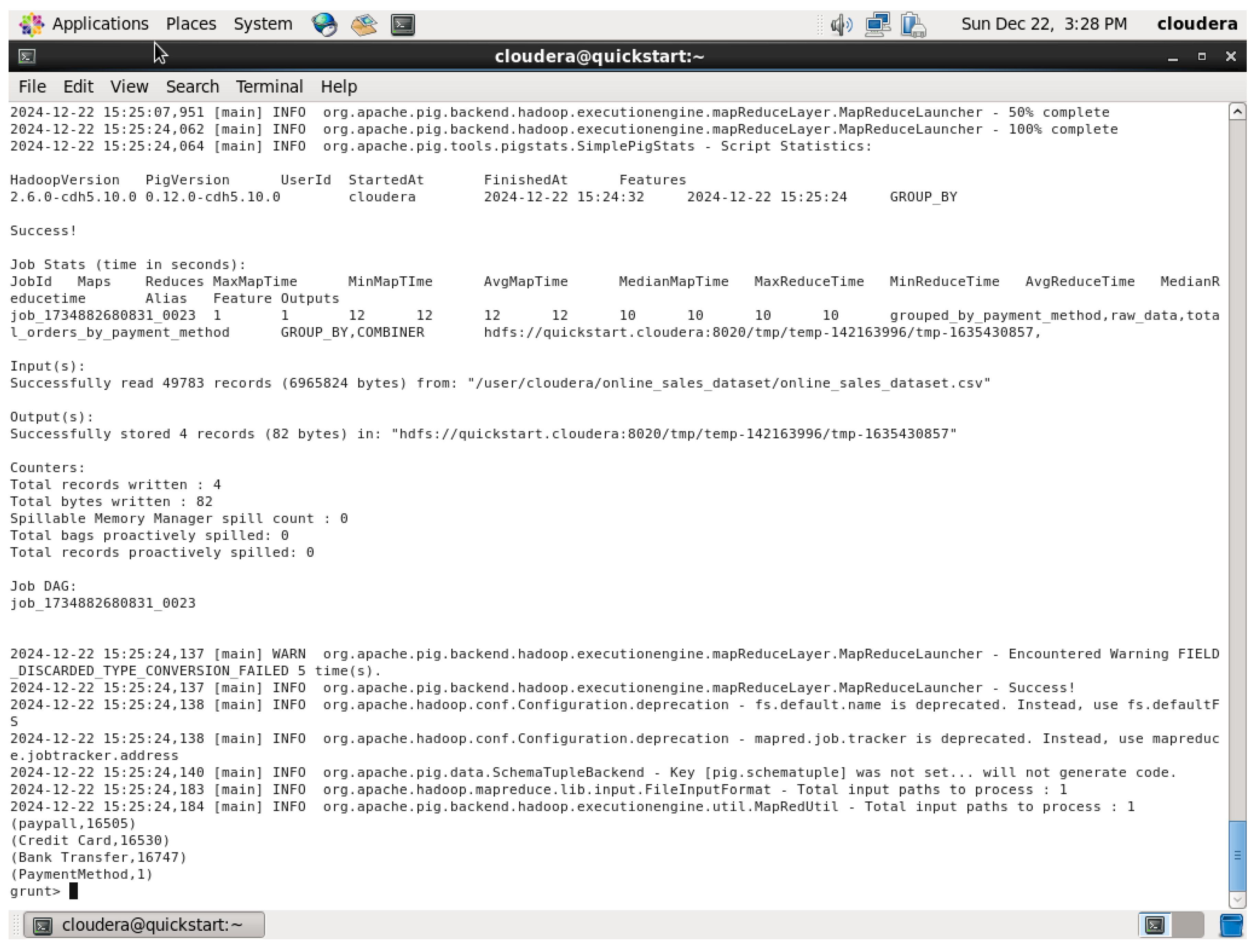
First, it loads the dataset, groups the data by the column “payment_method,” and understands the total orders coming for a particular payment method. Further, the COUNT function of the orders against every pay mode gives an insight into the most ordered kind of pay modes. Finally, the DUMP command prints out the number of total orders for each of the given payment methods.Each query is carried out with a combination of several Pig Latin operations, like LOAD, GROUP BY, FOREACH, SUM, AVG, ORDER BY and COUNT, in order to convert data into useful insights related to retail sales, which shows revenue, product sales, monthly trends, discount details and payment method trends.

8. Insights and Recommendations

Application of Machine Learning Algorithms to Predict Customer Preferences

Predicting customer preferences is vital for businesses to provide personalized experiences and maintain a competitive edge. The dataset provided contains 49,783 transactional records with 17 attributes, offering valuable insights into customer behaviors, product performance, and market trends. By applying machine learning techniques, businesses can extract actionable insights, enhance decision-making, and optimize marketing strategies.

A.

Supervised Learning

Supervised learning involves using labeled datasets to predict outcomes. Techniques like regression, classification, and decision trees can be applied to identify customer preferences.

Algorithms and Applications:

• Linear Regression: Predicts average spending or sales trend based on the historical purchase data thereby helping businesses optimize the pricing and inventory planning. This will forecast future sales for specific products or categories (Alizamir, Bandara, Eshragh, & Iravani, 2022).
• Decision Trees and Random Forests: Classifies customer preferences by analyzing features like product categories, payment methods, and return status, enabling targeted marketing (Ravi, 2024). It also segments them based on categories, discounts, or payment methods which facilitates personalized marketing and product recommendations.
• Support Vector Machines (SVM): According to Alizamir, Bandara, Eshragh, & Iravani, (2022), It distinguishes between high-value and low-value customers based on transactional attributes which aids in prioritizing customer retention efforts for high value segments.

B.

Unsupervised Learning

Unsupervised algorithms analyze unlabeled data to identify hidden patterns and relationships.

Algorithms and Applications:

• K-Means Clustering: Groups customers based on their purchase behavior (e.g., categories, discounts used, frequent buyers vs occasional shoppers, etc), facilitating segmentation for targeted promotions. K-means clustering groups the customers based on spending habits and preferences.
• Principal Component Analysis (PCA): Reduces data complexity by simplifying mutli-dimensional transactional data while preserving key relationships, aiding in visualizing and identifying customer behaviour trends (Roychowdhury, Alareqi, E., & Li., 2021)
• DBSCAN: Detects anomalies in transaction data, such as unusual purchase volumes or fraudulent activities. This thus enhances fraud prevention and efficiency of operation. DBSCAN can highlight outliers in buying patterns (Roychowdhury, Alareqi, E., & Li., 2021)

C.

Reinforcement Learning

Reinforcement learning (RL) optimizes customer engagement by interacting with and learning from the environment. It can adapt recommendations during live interactions.

Algorithms and Applications:

• Q-Learning: In accordance with Vallarino, D (2023), Recommends personalized products in real-time, adapting to customer preferences based on purchase history which boost the conversion rates and customer engagement.
• Deep Q-Networks (DQNs): Leverages neural networks to suggest products dynamically during active browsing sessions. It also personalizes promotions or recommendations in e-commerce platforms (Vallarino, D., 2023).
• Multi-Agent Reinforcement Learning (MARL): Coordinates promotional campaigns across multiple platforms to optimize customer reach thus ensures cohesive marketing efforts and resource allocation.

D.

Deep Learning

Deep learning models analyze large, complex datasets to uncover intricate patterns.

Algorithms and Applications:

• Convolutional Neural Networks (CNNs): With reference to Roychowdhury, Li, Alareqi, E., Pandita, Liu, & Soderberg (2020), Analyzes visual data from product images for aesthetic preferences to predict customer interest in specific designs or features. This helps in recommending visually appealing products to customers.
• Recurrent Neural Networks (RNNs): Forecasts customer preferences over time by analyzing sequential transaction data, such as repeat purchases. Therefore, this aids inventory planning and tailored marketing campaigns.
• Autoencoders: Detects deviations and unusual customer preferences or behaviors, enabling proactive responses to market shifts and emerging trends and concerns (Roychowdhury, Li, Alareqi, Pandita, Liu, & Soderberg., 2020)

Benefits and insights:

Implementing the ML algorithms significantly enhances business operations and customer satisfaction. By providing personalized product suggestions and targeted strategies, these algorithms improve the overall customer experience, fostering satisfaction and loyalty. Furthermore, accurate predictions streamline the inventory management, minimizing wastage and improving the operational efficiency. Advanced analytics further enable businesses to gain scalable insights into behaviour of customers, uncovering trends and patterns that support long-term growth and competitive advantage. Integrating these ML models with big data tools like Hive, Spark or Impala transforms the raw data into valuable resources for informed decision

-making and strategic planning, positioning ventures as leaders in their markets.

Recommendations and future research opportunities:

Based on the Online sales dataset and the findings, this section covers the tailored recommendations for leveraging Hive, Pig, and Impala to optimize sales and analysis and explores the future research directions in retail analytics.

HIVE

Use Case: Ideal for batch processing and querying large transactional datasets, particularly for historical sales analysis.

Advantages: Hive’s SQL-like querying capability allows for the generation of detailed sales reports and identifying long-term trends.

Recommendation: Hive can be used for generating weekly, monthly, and annual sales reports. It can also conduct product performance analyses by category or region. Furthermore, it also performs temporal analysis on revenue trends to support inventory planning and promotional strategies.

PIG

Use Case: Best suited for transforming unstructured or semi-structured data into structured formats suitable for analysis.

Advantages: Pig Latin scripting facilitates efficient data cleansing, transformation, and preprocessing.

Recommendation: Pig can be used to preprocess transaction logs by handling missing or inconsistent data. Aggregation of data for exploratory analysis, including identifying high-value customers or frequently returned products can also be done by Pig. Applying Pig for data enrichment tasks like appending external marketing or demographic data is also recommended.

IMPALA

Use Case: Optimal for real-time querying and interactive analytics.

Advantages: Impala delivers low-latency query execution, enabling dynamic analysis of online sales.

Recommendation: Using Impala to create real-time sales monitoring dashboards for actionable insights, tracking the top-selling products or regions during peak sales periods and supporting quick decision-making during flash sales or inventory shortages are some of the recommended usage by Impala.

Integration of tools:

According to Ibtisum, S (2020), the combined usage of Pig, Hive, and Impala creates a powerful workflow for managing and analyzing sales data. Pig is ideal for preprocessing raw data such as cleaning and organizing transaction logs into structured formats thus making the data ready for deeper analysis. Once the data is structured, Hive can be used to store and process it in batches, enabling detailed historical reporting and comprehensive trend analysis over time. For real time needs, Impala steps in to deliver quick insights on sales trends and customer behaviour, supporting immediate decisions.

A streamlined data pipeline can enhance the integration. Start by ingesting the raw transaction logs using Pig to clean and transform the data. The preprocessed data can then be stored in Hive, where it is analysed to generate reports and uncover deep insights into sales patterns and interactions of the customers (Ibtisum, S., 2020). Finally, leveraging Impala to build real time dashboards, allowing decision-makers to monitor ongoing sales trends and respond swiftly to changes in customer demand or market conditions.

Areas for Future Research:

Advanced Machine Learning Algorithms

According to Atitallah, Driss, Boulila & Ghézala (2020), In the realm of predictive analytics, algorithms like Gradient Boosting and Recurrent Neural Networks (RNNs) offer promising

solutions for forecasting seasonal sales trends and customer purchase probabilities. These models can help businesses anticipate demand fluctuations and tailor their strategies accordingly. Additionally, customer segmentation techniques such as Kmeans clustering are valuable for grouping customers based on their purchasing patterns and product preferences. This segmentation allows businesses to create targeted marketing campaigns thereby improving customer retention by addressing specific needs within each group.

Integration with IoT and Sensor Data

Real-time data integration through the use of IoT devices, like smart inventory trackers, can significantly enhance stock management by providing up-to-the-minute information on product availability. By incorporating these devices into a retail environment, businesses can ensure that they never run out of stock during peak demand periods. And furthermore, IoT-driven data can be leveraged to create more personalized shopping experiences. For instance, retailers can offer dynamic pricing or targeted promotions based on real-time insights into customer behavior and interactions within the store (Atitallah, Driss, Boulila, & Ghézala, H. B., 2020).

Scalability and Performance Optimization

As retail datasets continue to grow, it’s essential to explore scalable architectures that can handle the increasing data storage and processing demands. Cloud-based platforms like AWS or Azure are key players in this area, offering efficient solutions for scaling operations. These platforms ensure that businesses can store and process large amounts of data without compromising on performance. Additionally, optimizing SQL-like query execution in tools such as Hive and Impala is crucial for managing large datasets efficiently. Query optimization techniques can help reduce processing time and improve the overall performance of big data tools (Sarker, I. H. 2021).

Enhanced Data Visualization

With reference to Sarker, I. H. (2021), Interactive dashboards play a vital role in making complex sales data more accessible to decision-makers. Developing these dashboards enables retailers to explore their data in an intuitive, interactive way, thus aiding them uncover granular insights into customer behaviours and performance of sales. In addition, incorporating geospatial analytics into these visualizations can enhance regional analysis, provide valuable insights into local sales performance and logistics efficiency. By visualizing regional data, businesses can identify patterns, optimize the supply chains and better understand preferences of customers based on the locations.

This integrated approach ensures actionable insights into consumer behavior and supports the scalability of retail operations thus enabling businesses to adapt quickly to changing market conditions.

References

- Ali, A.H.; Abdullah, M.Z. A Survey on Vertical and Horizontal Scaling Platforms for Big Data Analytics. Int. J. Integr. Eng. 2019, 11. [CrossRef]
- Apache Pig Tutorial. (n.d.). https://www.tutorialspoint.com/apache_pig/index.htm.
- Alizamir, S., Bandara, K., Eshragh, A., & Iravani, F. (2022). A Hybrid Statistical-Machine Learning Approach for Analysing Online Customer Behavior: An Empirical Study. arXiv preprint arXiv:2212.02255.
- Atitallah, S. B., Driss, M., Boulila, W., & Ghézala, H. B. (2020). Leveraging Deep Learning and IoT big data analytics to support the smart cities development: Review and future directions. Computer Science Review, 38, 100303.
- Chiniah, A.; Mungur, A. On the Adoption of Erasure Code for Cloud Storage by Major Distributed Storage Systems. EAI Endorsed Trans. Cloud Syst. 2022, 7. [CrossRef]
- chandramouli, S. (2023, June 4). Dr. S. chandramouli Ph.D, PfMP on LinkedIn: Applications of bigdata in retail industries: Price optimization is a…. Linkedin.com. https://www.linkedin.com/posts/chandramoulisubramanian_applications-of-bigdata-in-ret ail-industries-activity-7071030446700056577-5p7B?originalSubdomain=lk.
- Cote, C. (2021, November 18). What Is Diagnostic Analytics? 4 Examples. Business Insights - Blog. https://online.hbs.edu/blog/post/diagnostic-analytics.
- Gartner. (2024, August 30). Gartner Reveals Three Technologies That Will Transform Customer Service and Support By 2028. Gartner. https://www.gartner.com/en/newsroom/press-releases/2023-08-30-gartner-reveals-three-t echnologies-that-will-transform-customer-service-and-support-by-2028.
- Giri, C.; Johansson, U.; Lofstrom, T. Predictive Modeling of Campaigns to Quantify Performance in Fashion Retail Industry. 2019 IEEE International Conference on Big Data (Big Data). United States; pp. 2267–2273.
- Guru, C.; Bajnaid, W. Prediction of Customer Sentiment Based on Online Reviews Using Machine Learning Algorithms. Int. J. Data Sci. Adv. Anal. 2023, 5, 272–279. [CrossRef]
- Hammond-Errey, M. (2023). Big Data Landscape Fuels Emerging Technologies. Routledge EBooks, 22–44. [CrossRef]
- HarshSingh. (2023, April 21). Apache Hive and its usecases - HarshSingh - Medium. Medium. https://medium.com/@harsh.b26/what-is-apache-hive-4ff82a9bb62c.
- Hive Tutorial. (n.d.). https://www.tutorialspoint.com/hive/index.htm.
- Impala Tutorial. (n.d.). https://www.tutorialspoint.com/impala/index.htm.
- Ibtisum, S. (2020). A Comparative Study on Different Big Data Tools.
- Invisibly. (2021, December 20). How Amazon Uses Big Data to Drive Innovation and Growth https://www.invisibly.com/learn-blog/how-amazon-uses-big-data-drive-innovation-and-gr owth/.
- Jankatti, S.; K., R.B.; S., R.; Meenakshi, M. Performance evaluation of Map-reduce jar pig hive and spark with machine learning using big data. Int. J. Electr. Comput. Eng. (IJECE) 2020, 10, 3811–3818. [CrossRef]
- Khader, M., & Al-Naymat, G. (2020). Density-based algorithms for big data clustering using MapReduce framework: A Comprehensive Study. ACM Computing Surveys (CSUR), 53(5), 1-38.
- Lin, J.; Dyer, C. Data-Intensive Text Processing with MapReduce. Synth. Lect. Hum. Lang. Technol. 2010, 3, 1–177. [CrossRef]
- Luu, H. (2021). Working with Apache Spark. Apress EBooks, 17–49. [CrossRef]
- Murugan, M. (2019, July 23). Sharing folders between Cloudera Quickstart VM and local desktop. RandomThoughts. https://kavinmaha.blog/2019/07/23/sharing-folders-between-cloudera-quickstart-vm-and- local-desktop/.
- Niu, Z.; He, B. (2019). Storage Technologies for Big Data. Encyclopedia of Big Data Technologies, 1591–1594. [CrossRef]
- Engineer, C.; Ravi, A. Optimizing Retail Operations: The Role of Machine Learning and Big Data in Data Science. Glob. Res. Dev. Journals 2024, 9, 1–10. [CrossRef]
- Raptis, T.P.; Passarella, A. A Survey on Networked Data Streaming With Apache Kafka. IEEE Access 2023, 11, 85333–85350. [CrossRef]
- Roychowdhury, S.; Alareqi, E.; Li, W. OPAM: Online Purchasing-behavior Analysis using Machine learning. 2021 International Joint Conference on Neural Networks (IJCNN). China; pp. 1–8.
- Roychowdhury, S., Li, W., Alareqi, E., Pandita, A., Liu, A., & Soderberg, J. (2020). Categorizing Online Shopping Behavior from Cosmetics to Electronics: An Analytical Framework. arXiv preprint arXiv:2010.02503.
- Sarker, I.H. Data Science and Analytics: An Overview from Data-Driven Smart Computing, Decision-Making and Applications Perspective. SN Comput. Sci. 2021, 2, 1–22. [CrossRef]
- Sharma, J.; Sharma, D.; Sharma, K. Retail Analytics to anticipate Covid-19 effects Using Big Data Technologies. 2021 IEEE Asia-Pacific Conference on Computer Science and Data Engineering (CSDE). Australia; pp. 1–6.
- Shi, Y. (2022). Big Data and Big Data Analytics. Advances in Big Data Analytics, 3–21. [CrossRef]
- Solanki, S.D.; Solanki, A.D.; Borah, S. (2022). Assimilate Machine Learning Algorithms in Big Data Analytics: Review. River Publishers EBooks, 81–114. [CrossRef]
- Tolulope, A.I. (2022). Descriptive Analytics Tools. Apress EBooks, 83–111. [CrossRef]
- Thakur, U.K. (2023) The Role of Machine Learning in Customer Experience. Advances in Business Information Systems and Analytics Book Series, 80–89. [CrossRef]
- Vallarino, D. Buy When? Survival Machine Learning Model Comparison for Purchase Timing. 3rd International Conference on Advances in Computing & Information Technologies. COUNTRY; .
- Yi, S. Walmart Sales Prediction Based on Machine Learning. Highlights Sci. Eng. Technol. 2023, 47, 87–94. [CrossRef]
- Zhai, Y.; Tchaye-Kondi, J.; Lin, K.-J.; Zhu, L.; Tao, W.; Du, X.; Guizani, M. Hadoop Perfect File: A fast and memory-efficient metadata access archive file to face small files problem in HDFS. J. Parallel Distrib. Comput. 2021, 156, 119–130. [CrossRef]
- Jhanjhi, N. Z., Gaur, L., & Khan, N. A. (2024). Global Navigation Satellite Systems for Logistics: Cybersecurity Issues and Challenges. Cybersecurity in the Transportation Industry, 49-67.
- Khan, M. R., Khan, N. R., & Jhanjhi, N. Z. (Eds.). (2024). Convergence of Industry 4.0 and supply chain sustainability. IGI Global.
- Ashraf, H.; Jhanjhi, N.Z.; Brohi, S.N.; Muzafar, S. (2024). A Comprehensive Exploration of DDoS Attacks and Cybersecurity Imperatives in the Digital Age. In Navigating Cyber Threats and Cybersecurity in the Logistics Industry (pp. 236-257). IGI Global Scientific Publishing.
- Qasim, M.; Mahmood, D.; Bibi, A.; Masud, M.; Ahmed, G.; Khan, S.; Jhanjhi, N.Z.; Hussain, S.J. PCA-Based Advanced Local Octa-Directional Pattern (ALODP-PCA): A Texture Feature Descriptor for Image Retrieval. Electronics 2022, 11, 202. [CrossRef]
- Lim, M.; Abdullah, A.; Jhanjhi, N. Performance optimization of criminal network hidden link prediction model with deep reinforcement learning. J. King Saud Univ. Comput. Inf. Sci. 2021, 33, 1202–1210. [CrossRef]
- Ashfaq, F.; Jhanjhi, N.Z.; Khan, N.A.; Muzafar, S.; Das, S.R. (2024, March). CrimeScene2Graph: Generating Scene Graphs from Crime Scene Descriptions Using BERT NER. In International Conference on Computational Intelligence in Pattern Recognition (pp. 183-201). Singapore: Springer Nature Singapore.
- JingXuan, C.; Tayyab, M.; Muzammal, S.M.; Jhanjhi, N.Z.; Ray, S.K.; Ashfaq, F. Integrating AI with Robotic Process Automation (RPA): Advancing Intelligent Automation Systems. 2024 IEEE 29th Asia Pacific Conference on Communications (APCC). Indonesia; pp. 259–265.
- Saeed, S.; Jhanjhi, N.; Abdullah, A.; Naqvi, M. Current Trends and Issues Legacy Application of the Serverless Architecture. Int. J. Comput. Netw. Technol. 2013, 6, 100–108. [CrossRef]
- Brohi, S. N., Jhanjhi, N. Z., Brohi, N. N., & Brohi, M. N. (2023). Key applications of state-of-the-art technologies to mitigate and eliminate COVID-19. Authorea Preprints.
- Zaman, D. N., & Memon, N. A. (2007). Pakistan lags behind in Technical Textiles. Journal of Management and Social Sciences, 3(2), 120-127.
- Zaman, N., Khan, A. R., & Salih, M. Designing of Energy aware Quality of Service (QoS) based routing protocol for Efficiency Improvement in Wireless Sensor Network (WSN).
- Humayun, M.; Jhanjhi, N.; Hamid, B.; Ahmed, G. Emerging Smart Logistics and Transportation Using IoT and Blockchain. IEEE Internet Things Mag. 2020, 3, 58–62. [CrossRef]
Disclaimer/Publisher’s Note: The statements, opinions and data contained in all publications are solely those of the individual author(s) and contributor(s) and not of MDPI and/or the editor(s). MDPI and/or the editor(s) disclaim responsibility for any injury to people or property resulting from any ideas, methods, instructions or products referred to in the content. |
© 2025 by the authors. Licensee MDPI, Basel, Switzerland. This article is an open access article distributed under the terms and conditions of the Creative Commons Attribution (CC BY) license (http://creativecommons.org/licenses/by/4.0/).
Copyright: This open access article is published under a Creative Commons CC BY 4.0 license, which permit the free download, distribution, and reuse, provided that the author and preprint are cited in any reuse.