Submitted:
03 December 2025
Posted:
05 December 2025
You are already at the latest version
Abstract
In this paper we present a method to get the prime counting function p(x) and other arithmetical functions than can be generated by a Dirichlet series, first we use the general variational method to derive the solution for a Fredholm Integral equation of first kind with symmetric Kernel K(x,y)=K(y,x), after that we find another integral equations with Kernels K(s,t)=K(t,s) for the Prime counting function and other arithmetical functions generated by Dirichlet series, then we could find a solution for π(x) and \( \sum_{n \le x} a(n) = A(x) \), solving δJ[ϕ]=0 for a given functional J, so the problem of finding a formula for the density of primes on the interval [2,x], or the calculation of the coefficients for a given arithmetical function a(n), can be viewed as some “Optimization” problems that can be attacked by either iterative or Numerical methods (as an example we introduce Rayleigh-Ritz and Newton methods with a brief description) Also we have introduced some conjectures about the asymptotic behavior of the series \( \Xi_n(x) = \sum_{p \le x} p^{\,n} = S_n(x)\ \) for n>0 , and a new expression for the Prime counting function in terms of the Non-trivial zeros of Riemann Zeta and its connection to Riemman Hypothesis and operator theory.
Keywords:
PNT (prime number theorem)
; variational calculus
; maxima and minima
; integral transforms
MSC: 11A41; 11Z05; 44-02; 44A05; 44A99
1. Variational Methods in Number Theory
It was Euler, in the problem of “Brachistochrone” (shortest time) or curve of fastest descent, who introduced the preliminaries of what later would be called, “Calculus of Variations”, he solved the problem minimizing the integral below, where “t” is the time employed by the particle to go from (0,0) to another point on the plane (x, y) below (0,0), using Newtonian mechanics he found the expression:
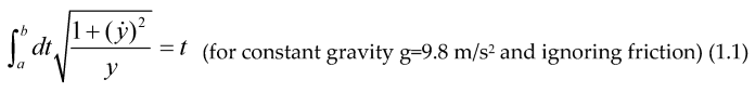
Then he got that the minimum of the integral above was a differential equation describing a cycloid, later Lagrange used this Calculus of Variations to describe the mechanics of a particle introducing the Lagrangian and the action functional S, whose extremum gave precisely the equations of motion for the particles:
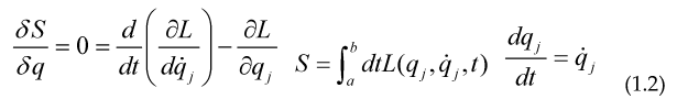
The equations above are the Euler-Lagrange equations of motion for the system defined by the Lagrangian L, this formulation is equivalent to Newton second law, although its use is more extended, as you only need to know the Kinetic part of the particle (usually of the form ) and a potential V related to the force is the force of the system, Here Q is an Hermitian Matrix.
Now we can ask ourselves if we can generate a similar Variational principle for number theory, for the case of a Fredholm equation of second kind, with K(x,y)=K(y,x) we have:

Taking the functional derivative.
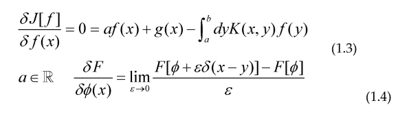
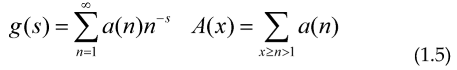
So we have derived for this especial case the Euler-Lagrange equation for this Integral equation, for the cases of the prime counting function and an arithmetical function that can be generated via Dirichlet series of the form:
We can give the 2 Functional, so their maximum or minimum are precisely some integral equations defining these arithmetical functions: (a=0)
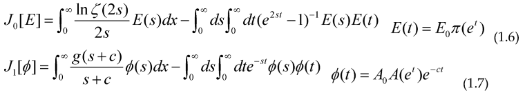
Minimizing these Functional with respect to E(s) and φ(s) and making the change of variable t=ln(x) we get the usual integral equation for π(x) and A(x) namely:

With c>0 and s>1/2 (the election of g(s+c) and 2s inside the second integral is to avoid the singularities inside the integrals due to a pole of the Riemann zeta function at s=1), this allows us to study the prime counting function and other arithmetical functions by using the Optimization techniques, including some iterative methods (gradient-descent, Newton method…) to calculate their “shape”, as an example of these iterative methods we can get the Maximum or Minimum for a given Functional:
2. On the Asymptotic Behavior of the Sums Over Primes, Beyond the Prime Number Theorem
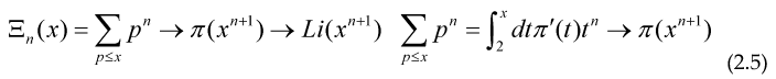
Now that we have given a method to obtain π(x) by Variational methods, after that we could study every sum over primes:
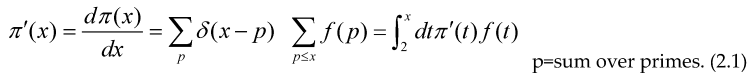
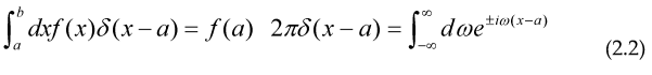
Where we have introduced the Dirac delta function with definition and properties:
Now we would be interested in some asymptotic behavior for the cases f(t)=tn as a conjecture, we have that the probability of a random integer number being prime is 1/ln(x) then we have the approximate (asymptotic) relationships:
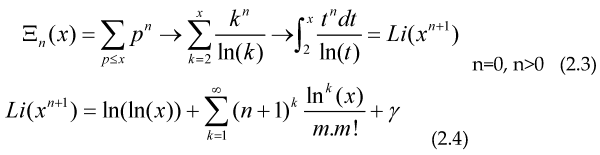
The last identity is found on tables for indefinite integrals, with γ the Euler-Mascheroni constant, for n=0 we get the Prime Number Theorem (PNT) , for n=1 we get the asymptotic relation:
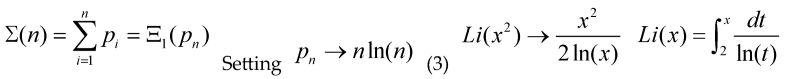
(3) is the asymptotic expression for the n-th prime, we use the European convention so Li(2)=0, expanding the Li(x2), keeping only the first term and using the prime number theorem to give an expression for n-th prime, we get:
For the case n=-1 the terms inside the sum over k cancel, so we get that the Harmonic prime series (as shown before, by Euler and others) diverges in the form ln(ln(x)) as x→∞, Or if our conjecture is valid, we can study the growth-rate of the series:
Differentiating both sides: With (PNT)
The last is how the derivative of the prime counting function behaves for big x, using the relation (2.4) with an function F(x) that is analytic near x=0 and has the limit , then the asymptotic expression for the sum:
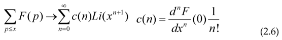
Where we have used the asymptotic notation meaning that
- ○
- Sum over primes:
For other convergent prime sums, first we use the identity:
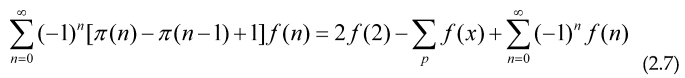
To obtain a relation between a prime series and an alternating series, valid when both, the alternating series and the sum over all primes for f(x) converge, the main purpose of this is that we can accelerate the convergence of the prime series using only a few values of n<100, as an example putting f(x)=x-s.
Where we have introduced the Prime Zeta function , The Euler (forward) transform for alternating series is given by the expression:
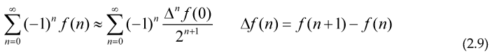
Euler method allows you to accelerate the convergence of an alternating series like (5) with general terms and providing that f(n)>f(n+1), if Euler transform is not good or converges worse than the initial series, we could use the backward Euler transform with the Backward difference operator ,the main purpose of using Euler transform is to be able to compute the expression . For a given f with an small error, knowing only a few values of the Prime counting function, so we can extract the behavior or approximate the sum for the series over all the primes, calculating the sum of the alternating series with general term (-1)nf(n), which is in general, easier to calculate, this expression to evaluate prime sums can also be applied to products.
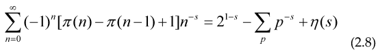
Even if the sum is divergent, we could use the functional equation for Riemann function relating so using the definition of the Prime zeta function in terms of the Möbius formula and Riemann Zeta:
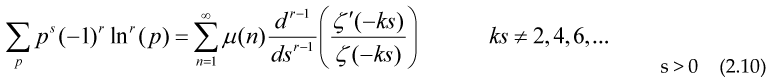
and r being a positive integer bigger than 1, we can consider the infinite sum on the right being the regularized value of the divergent prime sum on the left
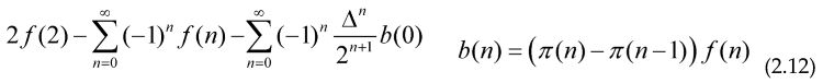
So expression (2.12) converges faster thant the sum
3. Sums Over Arithmetical Functions and Generalization of the Riemann-Weil Formula
In many important cases all the arithmetical functions which are useful in number theory has a Dirichlet series in the form , Where G(s) includes powers or quotients of the Riemann zeta function for example
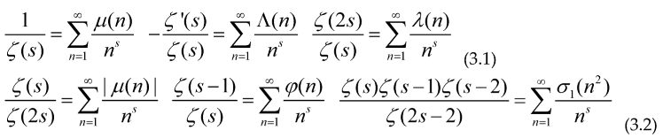
The definition of the functions inside (3.1) and (3.2) is as follows
- The Möbius function, if the number ‘n’ is square-free (not divisible by an square) with an even number of prime factors, if n is not squarefree and if the number ‘n’ is square-free (not divisible by an square) with an even number of prime factors.
- The Von Mangoldt function , in case ‘n’ is a prime or a prime power and takes the value 0 otherwise
- The Liouville function is the number of prime factors of the number ‘n’
- is 1 if the number is square-free and 0 otherwise
- , the meaning of is that the product is taken only over the primes p that divide ‘n’.
- is the divisor functionof order 1, it is equal to the sum of the divisors of the number ‘n’
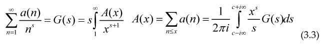
To obtain the coefficients of the Dirichlet series we can use the Perron formula
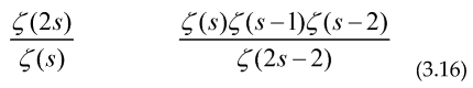
If the function G(s) includes powers and quotients of the Riemann zeta function we can use Cauchy’s theorem to obtain the explicit formulae for example
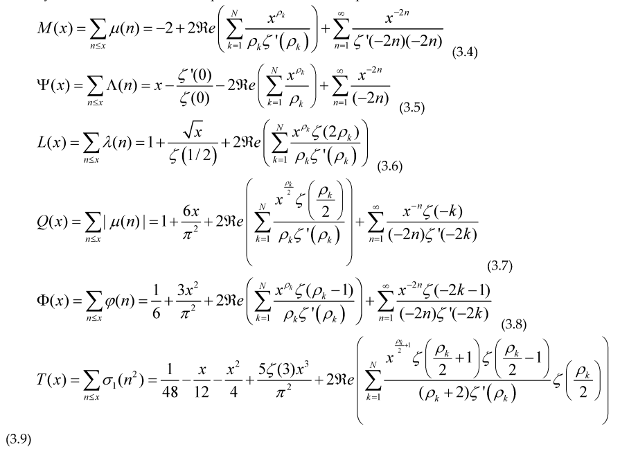
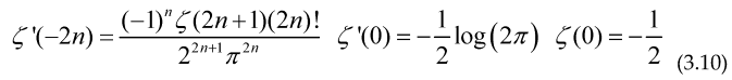
In all cases N must be taken in the limit , and the Real part is defined using the complex conjugate (linear) operator We have for the Riemann zeta function
The sum of an arithmetical function is an step function, therefore its derivative in distributional sense must satisfy , so if we take the derivative with respect to ‘x’ and make a change of variable inside every formulae (3.4) to (3.9).
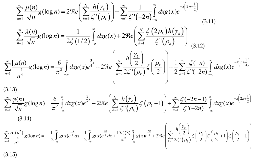
Where is an smooth test function, so it has a Fourier transform and the integral exists and is finite for every real number (positive or negative) ‘c’, and or depending on if the test function are even or not .
For the case of the Liouville function and the divisor function, there is no contribution due to the nontrivial Riemann zeroes -2,-4,-6,.… since the Dirichlet generating functions for these cases
Are Holomorphic on the region of the complex plane The sum over the Riemann zeros must be done as follows, we take the sum in pairs of zeros and , also for the imaginary part of the zeros, they must be summed in pairs and to avoid problems of convergence, that is the meaning of the expression inside each of the formulae (3.12) to (3.15). We have used the similar notation used in paper [3] to describe the sum over the nontrivial zeta zeros
These formulae are very similar to the Riemann-Weil explicit formula for the Chebyshev and Von Mangoldt functions
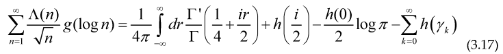
If we imopose that the function g(x) must be even we may write this function as for a certain function u(x), in this case we have a sum over in the form
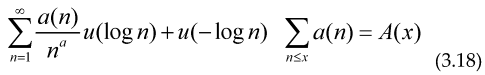
Although we have written expressions (3.12) to (.3.14) in terms of the imaginary part of the zeros, we can also express them as sums over zeros of the Riemann zeta function by doing the substitution
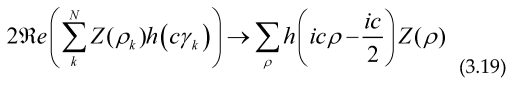
And the last sum on the right must be understood as a sum over the pairs of Riemann zeros and in increasing order,
Appendix A: A Conjecture Over Prime Numbers
Given the equation , where x,y,z are integers and , our cnejcture is this: we can always find three primes and so they satisfy the previous equation for example
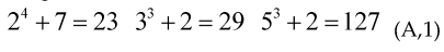
So for every exponent m there is a solution to the equation in primes (conjecture).
References
- Apostol Tom “Introduction to Analytic Number theory” ED: Springuer-Verlag, (1976).
- Avigad, J. Donnelly K, Gray D. and Raff P “A formally verified proof of the Prime Number Theorem” http://arxiv.org/abs/cs.AI/0509025.
- Baillie, R. “Experiments with zeta zeros and Perron formula” Arxiv: 1103.6226.
- Courant R. and Hilbert D. “Methods of Mathematical Physics” Vol 1, Ed: Interscience (1953).
- http://demonstrations.wolfram.
- Froberg, C.-E. On the Prime Zeta Function. BIT 8, 187–202, 1968.
- Hardy G.H “Divergent series”, Oxford, Clarendon Press (1949).
- Kendell A. Atkinson, “An introduction to numerical analysis” (2nd ed.), John Wiley & sons ISBN 0-471-50023-2 (1988).
- Odlyzko, A. M. and te Riele, H. J. J. Disproof of the Mertens Conjecture. J. reine angew. Math. 357, 138-160, 1985.
- Riemann B. “On the number of primes less than a Given Magnitude” Monthly reports of Berlin Academy (1859).
- Spiegel M. and Abellanas L “Mathematical Handbook of Formulas and Tables” ED: Mc Graw-Hill USA (1970) ISBN: 0-07-060224-7.
- Titchmarsh, E. C. “The Theory of Functions”, 2nd ed. Oxford, England: Oxford University Press, 1960.
Disclaimer/Publisher’s Note: The statements, opinions and data contained in all publications are solely those of the individual author(s) and contributor(s) and not of MDPI and/or the editor(s). MDPI and/or the editor(s) disclaim responsibility for any injury to people or property resulting from any ideas, methods, instructions or products referred to in the content. |
© 2025 by the author. Licensee MDPI, Basel, Switzerland. This article is an open access article distributed under the terms and conditions of the Creative Commons Attribution (CC BY) license (https://creativecommons.org/licenses/by/4.0/).
Copyright: This open access article is published under a Creative Commons CC BY 4.0 license, which permit the free download, distribution, and reuse, provided that the author and preprint are cited in any reuse.


