Submitted:
02 December 2025
Posted:
03 December 2025
You are already at the latest version
Abstract
This study takes the road closure problem as a case of combinatorial optimization and proposes a hybrid method that combines a Graph Neural Network (GNN) with a Genetic Algorithm (GA). The proposed approach uses the GNN to predict a closure potential score for each road (edge), and biases the GA’s initial solution genera-tion and mutation operations accordingly. In a virtual road network environment, the hybrid method reduced average travel time by approximately 3% compared to using GA alone. These results suggest that combining learning-based heuristics with evolutionary search can be an efficient and practically viable approach to solving combinatorial optimization problems.
Keywords:
combinatorial optimization
; genetic algorithm
; graph neural network
; learning-guided search
; road network optimization
1. Introduction
In real-world decision-making, various problems require selecting an optimal option under limited resources, and many of these problems can be formulated as combinatorial optimization tasks. This study focuses on the road closure problem, a representative combinatorial optimization problem. The road closure problem is based on Braess’s paradox, which suggests that removing specific road segments may paradoxically reduce overall network congestion. The task is to determine which road(s) to close to improve network performance, constituting a non-intuitive yet practically important variant of network design problems.
The road closure problem is classified as NP-hard, with a search space that grows exponentially with network size. As the scale increases, obtaining optimal solutions in polynomial time becomes infeasible; thus, approximation or heuristic-based approaches are essential for practical applications. A variety of metaheuristic methods, such as Genetic Algorithms (GA), Simulated Annealing (SA), Ant Colony Optimization (ACO), and Particle Swarm Optimization (PSO), have been applied to road network design and closure problems [1,2,3,4,5,6,7,8]. However, these traditional metaheuristics exhibit several limitations:
- high sensitivity to the quality of the initial solution;
- substantial computational cost when objective values rely on simulation-based evaluations such as SUMO; and
- insufficient exploitation of structural information inherent in network topology [9].
As a result, both search efficiency and solution quality degrade in large-scale or structurally complex networks.
Recently, there has been growing interest in combining deep learning–based heuristics with metaheuristic search for combinatorial optimization. In particular, Graph Neural Networks (GNNs) have demonstrated strong capability in learning structural patterns in graphs, and have been applied to problems such as the Traveling Salesman Problem (TSP), Vehicle Routing Problem (VRP), graph cuts, and network design within the frameworks of neural combinatorial optimization, learning-guided heuristics, and GNN-guided search. Many of these approaches use GNNs to predict node or edge scores, which are then used to construct complete solutions via greedy or beam-search procedures [10,11,12,13,14,15,16].
However, such end-to-end solution-generation approaches suffer from several structural limitations:
- instability when dealing with discrete and sparse solution spaces;
- degraded performance in gradient-free environments; and
- loss of the global exploration capability inherent to metaheuristic search.
These issues are particularly pronounced in road network problems, where objective evaluation is performed through SUMO and therefore exhibits expensive, black-box characteristics. In such settings, purely learning-based end-to-end search often becomes impractical.
In contrast, guiding specific operations of a metaheuristic with GNN-based probabilistic biases—without letting the GNN directly generate full solutions—offers a potential remedy to these limitations. Nevertheless, this hybrid strategy has been scarcely explored in transportation network applications, including the road closure problem. In particular, the idea of injecting GNN-derived structural bias into GA initialization or mutation operations is seldom reported in the literature, and its effectiveness has rarely been evaluated in simulation-based environments.
To address the limitations of existing metaheuristic approaches for road closure optimization, this study proposes a hybrid GA+GNN optimization framework that integrates the structural pattern-learning capabilities of GNNs with the global exploration ability of GA. The contributions of this work are summarized as follows:
- GNN-guided initialization and mutation via structural probabilistic bias: The GNN does not generate full solutions; instead, it biases edge-selection probabilities during initial population generation and mutation operations through a softmax-based strategy.
- Empirical evaluation of learning-guided evolutionary search: Using a SUMO-based microscopic traffic simulator and a fixed OD demand scenario, we quantitatively compare GA alone and the proposed GA+GNN approach under equal evaluation budgets.
- Analysis of the effect of GNN integration across GA components (init / mutation / both): By comparing different GNN usage modes, we provide methodological insights into which stages of GA benefit most from learning-based guidance.
Using a virtual road network and a SUMO-based simulation environment, this study evaluates and analyzes the improvement in average travel time achieved by the proposed hybrid method relative to a baseline GA under identical evaluation constraints.
2. Methods
This study addresses a combinatorial optimization problem in which a subset of roads (edges) in a road network is closed so as to minimize overall traffic performance under a given demand scenario. As the objective function, we use the average travel time measured by the Simulation of Urban MObility (SUMO) microscopic traffic simulator [17,18].
The objective value for a solution S is defined as
where is the travel time of vehicle i, and N is the number of vehicles. The primary goal of this study is to minimize . To this end, we apply a genetic algorithm (GA)–based search method that evaluates various combinations of road closures and efficiently explores combinations that minimize average travel time. In particular, we implement a hybrid optimization scheme by combining a graph neural network (GNN) that learns the closure effect of each road and incorporates this information into the initialization and mutation stages of the search process to improve search efficiency.
2.1. GA Representation and Search Space
To search over combinations of edge closures in the road network, we employ a binary-encoded GA. For each network, we first define the candidate edge set by excluding internal links (edges whose ID starts with “:” or whose attribute function="internal") and edges with zero lanes from the SUMO network, as well as a set of pre-specified protected edges that are never allowed to be closed.
A solution S is represented as a binary vector over , where is interpreted as closing edge e and as keeping it open. The number of closed edges
is upper-bounded and restricted to the range . After mutation, we always clamp k back into this range to satisfy the constraint.
2.2. Traffic Demand and Simulation Settings
The traffic demand used in this study directly follows the route/trip definitions linked in the SUMO configuration file sim.sumocfg, with a total of vehicles injected into the network. All vehicles share the same origin–destination (OD) pair so as to emulate peak demand concentrated along a specific corridor. Departure times and routes are taken from the pre-defined values in the SUMO route file, and the GA only modifies the edge closure combination while keeping the demand fixed when evaluating changes in average travel time. The virtual road network used in all experiments is shown in Figure 1, where nodes represent intersections and directed edges represent road segments.
If the number of arrived vehicles recorded in tripinfo.xml falls short of the scenario demand, the solution is regarded as unrealistic (i.e., some vehicles fail to depart or arrive), and a large penalty is assigned.
Objective function evaluation is performed via SUMO simulation. For a given solution corresponding to a closed-edge set S, we generate an additional file that marks each edge in S with the closingReroute attribute, run SUMO in non-GUI mode with reroute-period = 30 s and a maximum of simulation steps, and record the results. Teleporting is completely disabled by setting time-to-teleport = -1 and time-to-teleport.highways = -1. After the simulation finishes, we extract the travel time (duration) of each vehicle from tripinfo.xml, compute the average travel time , and use it as the fitness value in the GA.
In implementation, the objective value is average travel time; however, since the number of vehicles in each scenario is fixed ( vehicles in the network), minimizing average travel time is equivalent to minimizing total travel time. In the following cases, the solution is deemed unrealistic and assigned a large penalty value :
- (i)
- tripinfo.xml is not generated;
- (ii)
- any vehicle is recorded with vaporized="true";
- (iii)
- the number of vehicles recorded in tripinfo.xml is smaller than the scenario demand size; or
- (iv)
- no valid duration values are obtained at all.
2.3. Genetic Algorithm Settings
The GA population size is set to 24, and the number of generations is fixed to 15. For each condition (network and algorithm combination), we conduct 10 independent runs using random seeds . For each seed, the same seed is used consistently for the Python and NumPy random number generators, GA initial population generation, and SUMO control.
Tournament selection is employed with a tournament size of 4, and at each generation, parents are chosen as tournament winners based on the current fitness values (average travel time).
For recombination, we use a uniform crossover operator on the binary representation. For each bit position, the bit is inherited from either parent with probability , and the crossover rate is set to .
Mutation is implemented as bit-flip mutation. Let n denote the number of candidate edges ; then each individual is assigned
mutation bits, where denotes rounding to the nearest integer.
For a given individual , we define the sets of open and closed edges as
We split the total number of mutation bits m into
and perform flips from (closing edges) and flips from (opening edges).
2.4. Policy GNN: Input Features and Dataset
To guide the GA search, we train a Policy GNN that estimates edge importance on the road network. For each network, we first construct the graph structure and policy dataset.
For every node v, we compute: (i) the number of incoming edges excluding external links as the in-degree, (ii) the number of outgoing edges as the out-degree, and (iii) a binary indicator specifying whether the node is a signalized intersection. These are used as 3-dimensional node features
Edge features are constructed as a 6-dimensional vector including edge length, number of lanes, speed limit, priority value, and binary indicators indicating whether the source/target nodes have traffic signals (from_tls, to_tls). Thus, the input to the Policy GNN is a directed graph with 3-dimensional node features and 6-dimensional edge features.
The policy dataset for each network consists of random edge-closure combinations. To build it, we run the policy dataset generation script in eight parts in parallel, with each part generating 125 samples using different random seeds; these are then merged into the final dataset. Each sample consists of a mask vector , representing the closed-edge set S, and the corresponding average travel time y from the SUMO simulation.
For each sample, the number of closed edges k is chosen uniformly at random as an integer in (network-specific), and then k distinct edges are sampled without replacement from to form S. Simulation settings and penalty rules for teleporting/non-arrival are identical to those used in GA evaluation. Under abnormal conditions such as simulation failure, teleporting, or insufficient arrivals, the label y is set to , so that such combinations are treated as highly undesirable solutions.
2.5. Policy GNN Architecture and Training
The Policy GNN is implemented as a GATv2-based graph neural network. First, a linear layer maps node features to node embeddings of hidden dimension 256. Then two GATv2Conv layers are applied sequentially, using edge features as edge attributes. Each GATv2Conv layer has four attention heads with 64 output dimensions per head, resulting in a 256-dimensional output per layer.
Finally, for each edge , we concatenate the source and target node embeddings with the edge feature vector to obtain
which is fed into a fully connected MLP (two hidden layers with 256 units and ReLU activations) to produce a scalar score . This score is interpreted as an indicator of the “risk of performance degradation” when closing that edge.
For training, the samples per network are randomly shuffled and split into a validation set and a training set, with approximately (at least 200 samples) used for validation and the rest for training (in our experiments, 200 validation and 800 training samples). We use AdamW as the optimizer with a learning rate of and weight decay of . The number of epochs is fixed to 60, and the random seed is set to 42.
As the loss function, we employ a margin ranking loss that exploits the rank information of the average travel time labels y. Specifically, we define “best” samples as those in the bottom of the travel time distribution and “worst” samples as those in the top , and randomly resample best/worst pairs in each epoch. Given edge scores for a sample , let
denote the number of closed edges (i.e., edges with ). For samples with , we define the set score
by averaging the scores of the edges with . With a margin , we minimize
for best samples and worst samples , thereby encouraging higher set scores for poor (large travel time) closure combinations and lower scores for good (small travel time) combinations. The validation loss is computed in the same way, and we select as the final Policy GNN the model parameters at the epoch with the lowest validation loss.
2.6. Score Normalization and GA Representation
After training, we use the Policy GNN for each network to precompute the scores for all candidate edges . These scores are interpreted as scalar risks of performance degradation upon closure. The GA represents individuals as binary vectors , where and denote closed and open edges, respectively. Let denote the permissible range of the number of closed edges per network; in this study, we set .
We normalize the Policy GNN scores as follows. For all candidate edges, we compute
and define standardized scores
If is very small, it is clamped to to avoid numerical instability. In the GA initialization and mutation stages, we then use softmax distributions based on to decide which edges to open/close.
We fix the GA representation mode to “variable,” allowing each individual to have a variable number of closed edges within . When generating initial individuals, we first draw an integer
uniformly for each individual.
2.7. GNN-Guided Initialization
In the GA+GNN mode, we define initialization logits for each edge as
and compute the corresponding probability distribution
where controls the strength of the GNN score, and is the softmax temperature (we use and in the experiments). We then sample k edges without replacement from according to the distribution to construct the initial closed set
and set
As can be seen, edges with smaller standardized scores (lower risk) have larger and thus higher probability of being included in the initial closed set, whereas edges with larger (higher risk) are less likely to be initially closed.
For the GA-only baseline (gnn-usage = none), we set for all edges, so that and the above softmax degenerates into a uniform distribution. In this case, initial individuals are constructed by randomly choosing k edges uniformly from , without any policy bias. (In the implementation, for modes that do not use the policy at all, there also exists a code path where bits are initialized uniformly with probability and then adjusted to satisfy .)
2.8. GNN-Guided Mutation
At generation t, when mutating an individual , we first set and compute m as in Eq. (3). We then define and as in Eq. (4) and split m into and as in Eq. (5).
In mutation modes that use the Policy GNN (gnn-usage ), for the open set we define
and compute
where controls the influence of policy scores during mutation (we use ). We then sample edges without replacement from according to and flip their bits from 0 to 1 (closing them).
Conversely, for the closed set , we define
and compute
and sample edges from according to , flipping their bits from 1 to 0 (opening them). As a result, edges with small (low risk) have relatively high probabilities in and tend to be closed more frequently, whereas edges with large (high risk) have high probabilities in and tend to be opened more frequently.
After applying mutation, we add a correction step to ensure that the number of closed edges remains within . If , we randomly select some currently closed edges and flip them to 0; if , we randomly select some open edges and flip them to 1, thereby satisfying the constraint.
In GA-only and “initialization-only” policy modes (gnn-usage , respectively), we use an implementation equivalent to setting all . In this case, and and reduce to uniform distributions over their respective sets, making mutation equivalent to simple random bit flips. Thus, the GA-only baseline uses completely random initialization and uniform mutation, while the GA+GNN method probabilistically biases “closing” decisions toward lower-risk edges and “opening” decisions toward higher-risk edges according to the Policy GNN scores.
2.9. Parallel Evaluation and Caching
At each generation, individual evaluations (simulation runs) are executed by running up to eight SUMO processes in parallel. When the same closure set S is requested multiple times (e.g., due to elitism or coincidentally identical individuals), we cache the fitness value using a sorted string representation of the closed-edge set as a key, so that SUMO simulations are not re-run for identical solutions, thereby reducing computational cost. The GA-only baseline and the GA+GNN method share the same GA settings and evaluation procedure; they differ only in whether Policy GNN scores are used in the initialization and mutation stages.
2.10. Statistical Analysis
For statistical analysis of performance, we use the best-so-far average travel time at the final generation for each seed as a single observation (sample size per mode). We first apply the Shapiro–Wilk test to each mode (none, init, mutation, both) and to the pairwise differences relative to the none mode (e.g., both − none). In all cases, the normality assumption is not rejected (e.g., none: , ; paired_diff(both − none): , ).
Nevertheless, given the small sample size (10) and in order to reduce the influence of outliers, we adopt the non-parametric Wilcoxon signed-rank test for mode comparison. We treat the GA-only mode without GNN (none) as the baseline and perform three paired comparisons with the init, mutation, and both modes, respectively. To mitigate inflation of Type I error due to multiple comparisons, we report Holm-adjusted p-values.
Additionally, we quantify effect sizes using the rank-based effect size r, Cliff’s delta, and paired-sample Cohen’s , and estimate confidence intervals for Cliff’s delta via bootstrap (). The confidence intervals of the mean average travel time per mode are also obtained via bootstrap with .
2.11. Implementation Details and Computing Environment
All experiments are conducted on a desktop environment running Microsoft Windows 11 Pro (version 10.0.26200). The hardware consists of a 12th Gen Intel Core i7-12700KF processor (12 cores, 20 threads) and 32 GB of memory; GPU acceleration is not used.
The implementation is based on Python 3.13.9. For deep learning, we use PyTorch 2.5.1 and PyTorch Geometric 2.7.0. Traffic simulations are performed with Eclipse SUMO 1.24.0. The versions of major libraries and the full list of dependencies are provided in the environment.yml file included in the public repository.
The overall simulation pipeline is summarized in Figure 2.
Finally, by quantitatively evaluating the improvement in average performance and search efficiency of the GA+GNN hybrid method over GA alone, we verify that the proposed approach provides substantial improvements for combinatorial optimization problems in complex traffic networks.
3. Results
Figure 3 shows the best-so-far average travel time by generation for GA only and GNN-guided GA (GA+GNN) under identical random seeds, number of generations, and population size. Each method was run for 15 generations under 10 different seeds, and in each generation 24 individuals were generated and evaluated. The performance metric for each generation was the best-so-far average travel time [s] at that generation. In the plot, solid lines indicate the mean over seeds, and shaded bands represent 95% bootstrap confidence intervals () around the seed mean. At the final generation (Gen 15), GA only achieved about 302.93 s (95% CI 299.45–306.03), whereas GA+GNN achieved about 293.33 s (95% CI 289.43–296.95), i.e., GA+GNN was lower by 9.6 s (3.17%). Based on the final value for each seed, GA+GNN outperformed GA only in all 10 seeds.
Table 1 summarizes the final performance of GA only and GA+GNN in terms of the mean final average travel time, the corresponding 95% confidence intervals, and the relative improvement of GA+GNN over GA only.
To further analyze where the GNN contributes within the GA–GNN hybrid scheme, we decomposed it into four modes: (1) none: GA only without any use of the GNN; (2) init: GNN used only in the initial population generation; (3) mutation: GNN used only in the mutation operator; and (4) both: GNN used in both initialization and mutation. Under otherwise identical conditions, comparison of the average travel time across modes showed a decreasing trend in the order none >init>mutation> both, with the both mode (GNN used in both initialization and mutation) achieving the lowest average travel time (Figure 4).
We conducted paired Wilcoxon signed-rank tests on the final average travel times for the 10 seeds. The difference between GA only (none) and GA+GNN (both) remained statistically significant even after Holm correction (, ), and for all 10 seeds GA+GNN yielded a lower average travel time than GA only.
To quantitatively assess this trend, we used the final average travel time for each seed to compare each mode against the no-GNN baseline (none) using paired Wilcoxon signed-rank tests. The init mode, which uses the GNN only in the initialization stage, reduced the average travel time by about 5.53 s (1.83%) on average relative to none, but this difference was not statistically significant after Holm correction (, ). In contrast, the mutation mode, which uses the GNN only in the mutation stage, reduced the average travel time by about 8.57 s (2.83%) relative to none, and this difference was statistically significant at the 0.05 level (, after Holm correction). The both mode, which uses the GNN in both initialization and mutation, reduced the average travel time by about 9.61 s (3.17%) relative to none and, as noted above, showed the strongest significance with after Holm correction.
In summary, the largest improvement was obtained when the GNN was applied in both the initialization and mutation stages; using it only in the mutation stage also produced a statistically significant improvement. By contrast, using the GNN only in the initialization stage showed an average improvement trend but did not reach statistical significance with the present sample size.
4. Discussion
In this study, we addressed a road-closure combinatorial optimization problem and proposed a hybrid method (GA+GNN) in which a GNN-based policy model guides the initial solution generation and mutation operations of a genetic algorithm. Experiments on virtual road network showed that, under an identical evaluation budget (number of generations, population size, and number of seeds), GA+GNN reduced the final average travel time by about 3% compared to GA alone. In the generation-wise average travel time curves, GA+GNN maintained consistently lower values from the early generations, exhibiting a tendency to outperform GA alone in both convergence speed and final solution quality. These results suggest that a learning-based GNN policy can meaningfully support GA search.
To better understand the mechanism by which the GNN contributes to GA performance, we decomposed the GA–GNN hybrid into four modes according to how the GNN is used: (1) none (GA only), (2) init (GNN used only for initial population generation), (3) mutation (GNN used only in the mutation operator), and (4) both (GNN used in both initialization and mutation). Based on the average travel time at generation 15, the results generally followed the pattern none > init > mutation > both.
These findings can be interpreted as follows.
- Effect of initialization (init). In the init mode, a subset of initial individuals is sampled from a distribution based on the GNN scores, rather than being fully random as in none. This mode consistently achieved lower average travel times than none, indicating that the edge-importance scores learned by the policy GNN are to some extent informative.
- Effect of mutation (mutation). The mutation mode, in which the GNN is used only in the mutation stage, performed better than init. This suggests that, rather than merely improving the initial solutions, biasing which bits are flipped more frequently during the generations using learned scores has a more direct impact on GA performance. Random mutation helps maintain a broad search space, but it is less effective at preserving and reinforcing promising structures. In contrast, GNN-guided mutation can be viewed as a kind of learned local search: it tends to close edges that are “better to close” more often, and to open edges that are “harmful when closed” more often, thereby steering the search. At the same time, if mutation probabilities for certain edges are overly biased, population diversity may decrease and the risk of premature convergence may increase; thus, it is important to balance the strength of the bias with sufficient randomness.
- Combined effect in the both mode. The both mode, which uses the GNN in both initialization and mutation, achieved the lowest average travel time among the four modes. This indicates that combining a high-quality initial population with directed local search allows the algorithm to reach good solutions more rapidly under a limited evaluation budget. However, the magnitude of the improvement is not overwhelmingly large, and the performance differences are likely to depend on network structure, demand settings, and parameter choices. It is therefore reasonable to view the design problem as deciding where in the algorithm and to what degree to introduce bias. Since the exploration–exploitation balance can shift depending on how strongly and in which stages (initialization/mutation) the bias is applied, a systematic comparison of such design choices is an important topic for future work.
The road-closure problem considered in this study can be interpreted as a prototypical combinatorial optimization problem defined on a graph, where the goal is to minimize a simulation-based objective function by making binary decisions on the graph. From this perspective, the proposed GA+GNN framework is not merely a problem-specific solution for a particular road network, but an instance of a more general design pattern: using a learned policy to bias metaheuristic search in graph-based combinatorial optimization. For example, if appropriate state representations and training data can be constructed, similar GNN guidance could be applied to other network design problems that involve binary or multi-valued decisions on edges or nodes, such as link opening/closure, capacity expansion, or facility location.
There are, however, limitations to the interpretation of the present results. Since the experiments were conducted on a single network and scenario, the fact that GNN-guided GA outperformed pure GA may be specific to the experimental setting, and it is difficult to draw general conclusions about the effectiveness of the proposed method. In addition, the demand scenario used in this study is a simplified one in which all vehicles share the same origin and destination nodes, which does not adequately capture the diverse OD patterns observed in real urban traffic. Under such a setting, demand is concentrated on specific bottleneck links, and the effect of edge-closure policies may be exaggerated or distorted compared to actual networks. In light of these limitations, this study points toward extending the analysis to multiple networks and demand conditions as an important direction for future work.
Author Contributions
Conceptualization, S.K. and J.P.; methodology, S.K.; software, S.K.; validation, S.K. and J.P.; formal analysis, S.K.; investigation, S.K.; writing—original draft preparation, S.K.; writing—review and editing, S.K. and J.P.; supervision, J.P. All authors have read and agreed to the published version of the manuscript.
Funding
This research received no external funding.
Institutional Review Board Statement
Not applicable. The study did not involve humans or animals and was based solely on computer simulations of virtual road network.
Informed Consent Statement
Not applicable. The study did not involve human participants.
Data Availability Statement
The code and data used in this study are openly available on GitHub at https://github.com/soyoon326/gnn-ga-road-closure.
Acknowledgments
The author thanks J.P. for helpful comments on earlier versions of this work. During the preparation of this manuscript, the author used ChatGPT (GPT-5.1, OpenAI) for assistance with language editing, code refactoring, and organization of the manuscript. The author has reviewed and edited the output and takes full responsibility for the content of this publication.
Conflicts of Interest
The author declares no conflicts of interest. The funders had no role in the design of the study; in the collection, analyses, or interpretation of data; in the writing of the manuscript; or in the decision to publish the results.
Abbreviations
The following abbreviations are used in this manuscript:
| GA | Genetic Algorithm |
| GNN | Graph Neural Network |
| SUMO | Simulation of Urban MObility |
| ATT | Average Travel Time |
| CI | Confidence Interval |
References
- Friesz, T.L.; et al. A Simulated Annealing Approach to the Network Design Problem with Variational Inequality Constraints. Transportation Science 1992, 26, 18–26. [Google Scholar] [CrossRef]
- Friesz, T.L.; et al. The Multiobjective Equilibrium Network Design Problem Revisited: A Simulated Annealing Approach. European Journal of Operational Research 1993, 65, 44–57. [Google Scholar] [CrossRef]
- Durán-Micco, J.; Vansteenwegen, P. A Survey on the Transit Network Design and Frequency Setting Problem. Public Transport 2022, 14, 155–190. [Google Scholar] [CrossRef]
- Ceylan, H.; Bell, M.G.H. Traffic Signal Timing Optimisation Based on Genetic Algorithm Approach, Including Drivers’ Routing. Transportation Research Part B: Methodological 2004, 38, 329–342. [Google Scholar] [CrossRef]
- Xu, T.; et al. Study on the Continuous Network Design Problem Using Simulated Annealing and Genetic Algorithm. Expert Systems with Applications 2009, 36, 2735–2741. [Google Scholar] [CrossRef]
- Ma, W.; Cheu, R.L.; Lee, D.-H. Scheduling of Lane Closures Using Genetic Algorithms with Traffic Assignments and Distributed Simulations. Journal of Transportation Engineering 2004, 130, 322–329. [Google Scholar] [CrossRef]
- Chien, S.I.J.; Tang, Y. Scheduling Highway Work Zones with Genetic Algorithm Considering the Impact of Traffic Diversion. Journal of Advanced Transportation 2014, 48, 287–303. [Google Scholar] [CrossRef]
- Mao, X.; Jiang, X.; Yuan, C.; Zhou, J. Modeling the Optimal Maintenance Scheduling Strategy for Bridge Networks. Appl. Sci. 2020, 10, 498. [Google Scholar] [CrossRef]
- Agushaka, J.O.; Ezugwu, A.E. Initialisation Approaches for Population-Based Metaheuristic Algorithms: A Comprehensive Review. Appl. Sci. 2022, 12, 896. [Google Scholar] [CrossRef]
- Vinyals, O.; Fortunato, M.; Jaitly, N. Pointer Networks. In Proceedings of the 28th International Conference on Neural Information Processing Systems (NeurIPS; 2015; pp. 2692–2700. [Google Scholar] [CrossRef]
- Bello, I.; Pham, H.; Le, Q.V.; Norouzi, M.; Bengio, S. Neural Combinatorial Optimization with Reinforcement Learning. arXiv 2016, arXiv:1611.09940. [Google Scholar] [CrossRef]
- Kool, W.; van Hoof, H.; Welling, M. Attention, Learn to Solve Routing Problems! In Proceedings of the International Conference on Learning Representations (ICLR, 2019. [Google Scholar] [CrossRef]
- Dai, H.; Khalil, E.; Zhang, Y.; Dilkina, B.; Song, L. Learning Combinatorial Optimization Algorithms over Graphs. In Proceedings of the 30th International Conference on Neural Information Processing Systems (NeurIPS; 2017; pp. 6348–6358. [Google Scholar] [CrossRef]
- Li, Z.; Chen, Q.; Koltun, V. Combinatorial Optimization with Graph Convolutional Networks. In Proceedings of the 32nd International Conference on Neural Information Processing Systems (NeurIPS; 2018; pp. 537–546. [Google Scholar] [CrossRef]
- Gasse, M.; Chételat, D.; Ferroni, N.; Charlin, L.; Lodi, A. Exact Combinatorial Optimization with Graph Convolutional Neural Networks. In Proceedings of the 33rd International Conference on Neural Information Processing Systems (NeurIPS; 2019. [Google Scholar] [CrossRef]
- Cappart, Q.; Chételat, D.; Khalil, E.; Morris, C.; Lodi, A.; Veličković, P. Combinatorial Optimization and Reasoning with Graph Neural Networks. Journal of Machine Learning Research 2023, 24, 1–61. [Google Scholar] [CrossRef]
- Lopez, P.A.; Behrisch, M.; Bieker-Walz, L.; Erdmann, J.; Flötteröd, Y.-P.; Hilbrich, R.; Lücken, L.; Rummel, J.; Wagner, P.; Wiessner, E. Microscopic Traffic Simulation Using SUMO. In Proceedings of the 21st IEEE International Conference on Intelligent Transportation Systems (ITSC 2018), Maui, HI, USA, 4–7 November 2018; pp. 2575–2582. [Google Scholar] [CrossRef]
- Eclipse SUMO. Simulation of Urban MObility (SUMO), Version 1.24.0. Zenodo 2025. [Google Scholar] [CrossRef]
Figure 1.
Road network used in the experiments
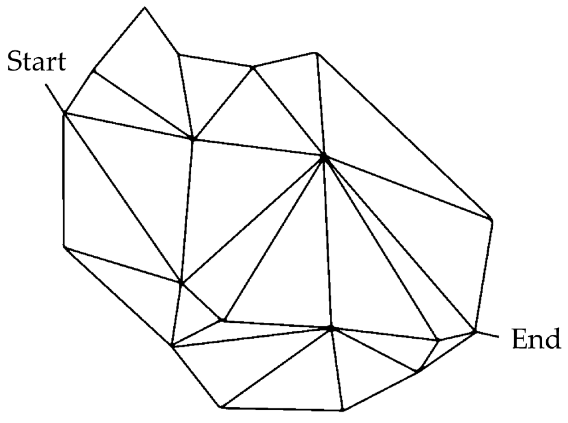
Figure 2.
Overall Pipeline of the Proposed GA+GNN-Based Road-Closure Optimization Framework
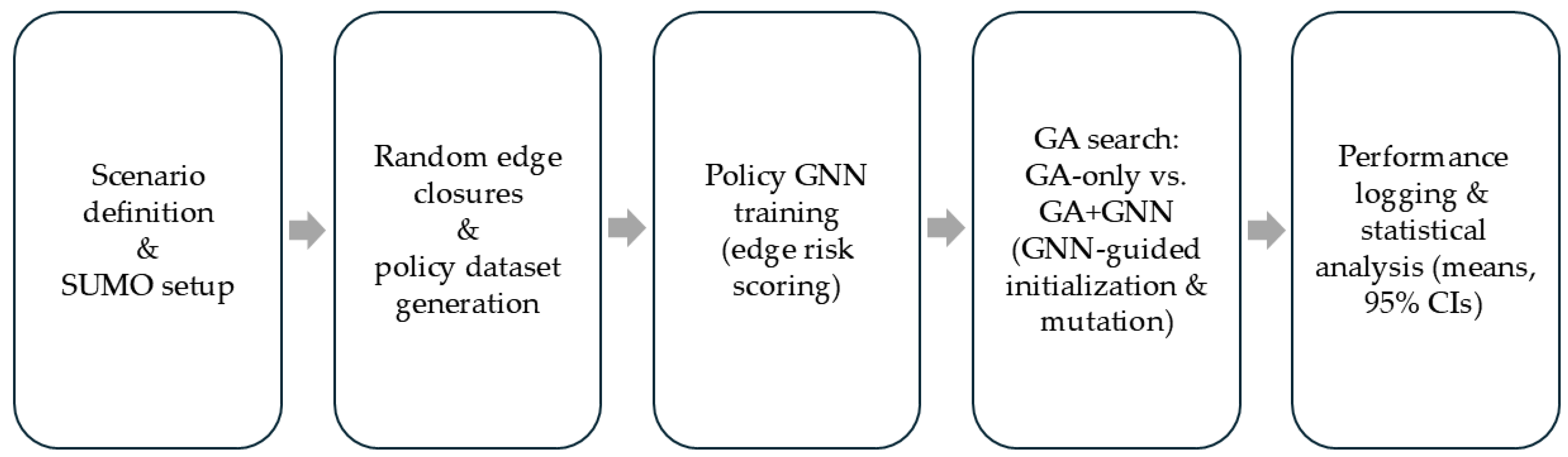
Figure 3.
Best-so-far average travel time by generation (GA vs. GA+GNN).
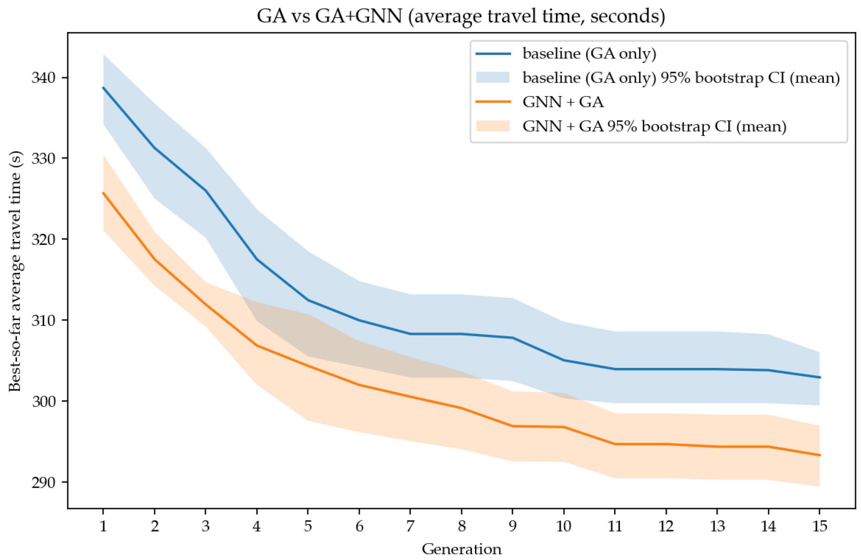
Figure 4.
Average travel time by GNN usage mode (none, init, mutation, both).
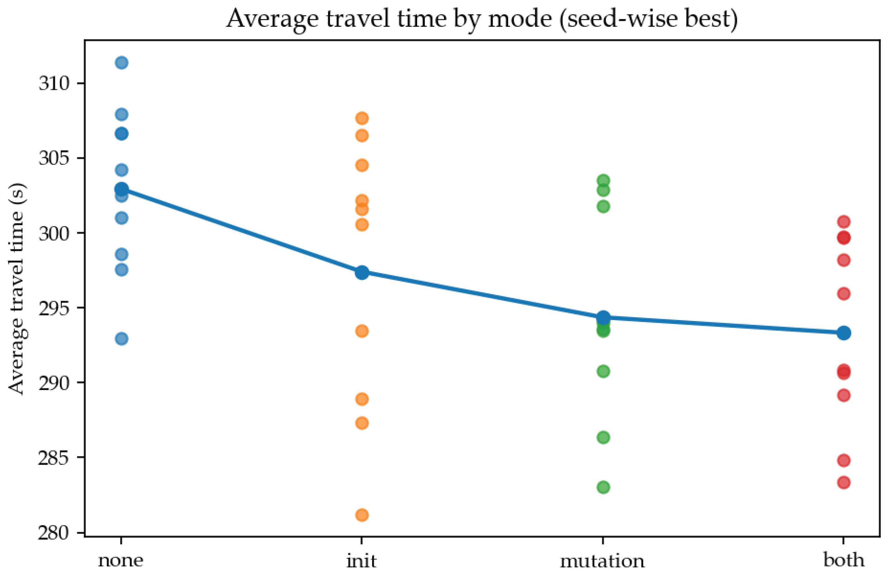

Table 1.
Final performance of GA only and GA+GNN (15 generations, 10 seeds).
| Method | Final average travel time [s] | 95% CI [s] | Improvement vs. GA only |
|---|---|---|---|
| GA only | 302.93 | 299.45–306.03 | – |
| GA+GNN | 293.33 | 289.43–296.95 | s (%) |
Disclaimer/Publisher’s Note: The statements, opinions and data contained in all publications are solely those of the individual author(s) and contributor(s) and not of MDPI and/or the editor(s). MDPI and/or the editor(s) disclaim responsibility for any injury to people or property resulting from any ideas, methods, instructions or products referred to in the content. |
© 2025 by the authors. Licensee MDPI, Basel, Switzerland. This article is an open access article distributed under the terms and conditions of the Creative Commons Attribution (CC BY) license (http://creativecommons.org/licenses/by/4.0/).
Copyright: This open access article is published under a Creative Commons CC BY 4.0 license, which permit the free download, distribution, and reuse, provided that the author and preprint are cited in any reuse.


