Quantitative Assessment of Greenhouse Gas Emissions in New Zealand Using Exploratory Data Analysis and Statistical Modelling Approaches

0.1. Background of Study

Greenhouse gases (GHGs), primarily carbon dioxide (CO₂), methane (CH₄), and nitrous oxide (N₂O), are critical components of Earth’s atmosphere and naturally plays a role in maintaining a stable climate. However, excessive GHGs have significantly changed the Earth’s atmosphere mainly due to human activity. This includes burning of fossil fuels, industrial processes, and agricultural activities. This results in increased concentrations of GHG in the atmosphere (Nunez, 2019). These elevated levels of GHG trap more heat, intensifying the greenhouse effect and causing a rise in global warming at an unprecedented rate (USGS, 2023).

Over recent decades, the continuous rise in GHG levels has been directly linked to climate change. This causes alarming consequences such as extreme weather events like hurricanes, heatwaves and droughts, have become more frequent and severe (Shivanna, 2022). Secondly, sea levels are on a rise due to melting ice caps and glaciers, endangering coastal communities and low-lying regions (Shivanna, 2022). These phenomena give rise to substantial threats to ecosystems and biodiversity, economies, and public health globally.

The implications of rising GHG levels extend beyond environmental concerns, affecting public health and social stability. Communities worldwide face challenges such as food supply uncertainty due to poor crop yields, increased respiratory and cardiovascular diseases caused by pollution, and forced migration due to climate-related disasters (Nguyen et al., 2023). Addressing this issue requires a thorough understanding of the trends and drivers of GHG emissions. By focusing on these aspects, targeted actions can be developed to mitigate the risks, adapt to changes, and promote sustainable development.

0.2. Problem Statement

The following list demonstrates the issues which this paper attempts to unveil:

• Greenhouse gas (GHG) concentrations continue to increase, significantly affecting sectors such as agriculture, transportation, and public health.
• Unpredictable weather patterns and climate-related disruptions are leading to reduced crop yields, transportation challenges, and increased health vulnerabilities.
• There is a lack of clear statistical insights to guide effective policies and actions to mitigate these issues.

Bringing these issues to light will provide a better understanding of the impacts which the nation’s efforts to combat climate change have on the greenhouse gas concentration in the air.

0.3. Objective

The objectives of this paper includes the following:

• To examine statistical data to uncover trends and patterns in greenhouse gas emissions.
• To determine the primary drivers behind the increase in GHG emissions over time.
• To evaluate the sectoral impacts of GHG emissions, with an emphasis on agriculture, transportation, and public health.
• To provide actionable insights that can inform policy making and sustainable development efforts.
• To support stakeholders, such as policymakers and environmental organizations, in addressing climate change through evidence-based strategies.

By following the objectives, this paper aims to help decision makers make better choices for the sake of a better, greener and cleaner future.

0.4. Parties Affected

The constant rise in GHG levels affects multiple sectors, including agriculture, transportation, industry, and public health. Each of these sectors faces unique challenges due to the increasing frequency and severity of climate-related disruptions.

In agriculture, harsh and unpredictable weather conditions (Yang et al., 2021) such as droughts, floods, and sudden temperature fluctuations, reduces crop yields in many farms, making farming less reliable. Crop yields drop drastically as vegetation struggles to adjust to these abrupt weather shifts. This consequently results in financial strain for farmers and jeopardizes food supply for populations. Additionally, the health and productivity of livestock are also affected, creating yet another challenge for agricultural sustainability (United States Environmental Protection Agency, 2020). These disruptions not only impact rural economies but also contribute to price volatility in global food markets.

Transportation faces similar challenges since severe weather events create hazardous conditions for commuters and freight. Frequent heavy downpour and slippery roads lead to congestion, delays, and even accidents (Gössling et al., 2023). This interrupts daily travel for individuals and the shipment of products. These delays lead to inefficiencies in the supply chain and financial setbacks for sectors that depend significantly on logistics (Faheem et al., 2024). Prolonged disruptions can also strain infrastructure, requiring costly repairs and upgrades.

Finally, the changing climate has a major effect on public health. Sudden changes in temperature (Yang et al., 2021) can lead to respiratory and cardiovascular diseases, especially in at-risk populations such as the elderly and children. Moreover, vector-borne diseases such as dengue and malaria become more prevalent with increasing temperatures, particularly in areas that were previously immune. These health issues put pressure on healthcare systems, escalate medical expenses, and diminish the overall quality of life for impacted groups.

0.5. Significance of Study

The aim of this research is to gain valuable insights that facilitate environmental advancement and promote sustainable ways of living. Analyzing the data and understanding the emissions patterns while identifying important elements is crucial for addressing the challenges posed by climate change. These findings are crucial for guiding efforts such as enhancing energy efficiency, promoting renewable energy, and reducing reliance on fossil fuels to secure a healthier environment and improved quality of life.

1.0. Literature Review

In this chapter, existing research on greenhouse gas (GHG) emissions relevant to New Zealand is summarised, including key contributing sectors, such as agriculture, manufacturing, transport and households. Covering evaluations of studies from 2007 to 2022, it assesses trends in emissions, what’s causing emissions, and how effective past interventions were, providing a basis for understanding and managing New Zealand’s GHG emissions.

1.1. Introduction to Greenhouse Gas Emissions

The challenge of trailing countries with a GHG developing world for the environment, in the same light, with the major emissions contributing to climate change and most as brooders to the sustainable development poses great concern for a country that comprises manufacturing, transportation, and agriculture as its core aspects.

This literature review evaluates two decades of research which focused on GHG originating from the primary sector, goods producing sector, and the service sector as well as households’ transportation sector and heating and cooling effects from the year 2007 to the year 2022. This describes the success of past interventions as well as explains the emission profile of New Zealand by sectors on the basis of statistical analysis, appropriate indicators and outcome of other authors’ studies. This provides a justification for GHG emission management strategies by this country (Stats NZ, 2024).

1.2. Variables of Interest in Previous Work

Since carbon emissions are in every country, it is possible to find activities that can be directed towards GHG emission per capita inNew Zealand. The following are the main factors that have been the focus of earlier research (Ritchie, 2020):

Agricultural Output: For emissions analysis within horticulture and arable farming for New Zealand’s primary sector, factors such as fertilizer application and irrigation, crop production output per hectare (or other land), and the number of livestock are essential. Such factors are useful in estimating GHG emissions from agricultural and related activities as livestock methane and soil management nitrous oxides are some of the greatest areas of concern (Leahy et al., 2021).

Industrial Activity Levels: For those industries which manufacture commodities some of the emissions determining factors include the amount of waste generated or even dumped, energy utilized (both gas and electricity), and production. For instance, these challenges are evident in manufacturing in relation to energy consumption, process emissions incurred from construction, waste management, incidentally reported in Stats NZ (2023).

Energy Consumption: It is the direct relationship between emissions with energy level handling in goods and services just like electricity and fossil fuels. Previous studies indicate a significant correlation between GHG emissions in relation to industrial activities that are energy intensive. It has been shown over time that variations in fuel types, trends in electrification, and the implementation of energy efficient practices has an effect on emissions trends (Ministry for the Environment, 2024).

Transportation Metrics: Metrics including fleet composition, fuel usage, and vehicle kilometres travelled are essential to emissions analysis for service businesses, especially the transportation, postal, and warehousing sectors. The use of private vehicles, commuter habits, and fuel type (such as petrol versus diesel) are important factors affecting emissions related to transportation within households (Ministry of Business, Innovation & Employment, 2016).

Heating/Cooling and Household Energy Use: Research on emissions from households often emphasizes energy consumption for heating and cooling, where elements like fuel type (for instance, natural gas or electricity) and seasonal variations (like winter heating spikes) impact emissions. The focus includes the impact of energy utilization infrastructural capacity on GHG emissions as well as other household activities such as use of electrical appliances (Rewiring Aotearoa, 2024).

1.3. Statistical Approach in Previous Work

In New Zealand, research on GHG emissions is associated with a number of statistical techniques aimed at predicting emissions, determining temporal patterns and major sources of emissions. Some of these methods include time series analysis, regression analysis, input-output analysis, emission factor models and geographic analysis.

Time-Series and Regression Analyses: The time-series analysis regression and the regression analysis of emissions are the methods used for analyzing the trends shown by the emissions and the variables affecting their trends. The analysis of times series methods are useful in determining seasonal cycles, long-term average trends and respective forecasts that take place between 2007 and 2022. This is important in agriculture since cropping and animal husbandry are seasonal activities resulting in emission changes (Tableau, n.d 2024).

Regression models provide additional substantiation by determining the drives of emissions in relation to energy, fertilizer and animal power employed. Our understanding of industry specific issues are further enhanced by multivariate regression techniques, which allow the investigators to isolate significant factors, allocating emissions to specified industries (Alchemer, 2021).

Input-Output Analysis: Input-output analysis is also very useful for examining greenhouse gas emissions given the linkages between different sectors. Based on emissions associated with output, this symmetry assesses whether emissions in one sector (e.g., manufacturing) affect emissions in another sector (e.g., transportation). Researchers can also identify emissions contributions indirectly by analyzing goods and services transfer between firms. This is especially useful for industries that deal with complex supply chains, including manufacturing and construction.

Emission Factor Models: Emission factor models use standardized emission coefficients for specific activities, such as fuel combustion or agricultural activities, to estimate emissions. Such a model is especially useful for analysing household emissions as it enables the calculation of total emissions with the help of activity-specific emission factors.

1.4. Findings of the Previous Work

Analysis of the contribution of emission sources and the effects of several intervention policies has produced essential insights within the literature on New Zealand’s GHG emissions in the past 15 years:

Primary Industries: The major contributor to emissions coming from the agricultural sector is methane emissions resulting from livestock and nitrous oxide emissions from the application of fertilizers. Even with advances in technology, it has been impossible for New Zealand’s agriculture sector to significantly reduce emissions without sacrificing production output levels. Because of the size and intensity of the sector, policies that have encouraged best practices in soil management and feeding regime changes have produced slight improvements rather than significant reductions (Tātai Aho Rau Learnz, 2016).

Goods-Producing Industries: Construction and manufacturing, particularly where they depend largely on non-renewable energy sources, account for a significant proportion of greenhouse gas emissions. The emissions from the construction industry fluctuate with the level of construction activity. The emissions from production and electricity generation are driven to some extent by energy policy and technological improvements, according to studies, with decreases currently noticed as a result of greater adoption of cleaner energy sources and energy-efficient devices (Infometrics, n. d.).

Service Industries: Emissions from transport, post, and storage activities have remained massive in the service sector. Investigations show that, as regards emissions in this sector, the single-most important contributor is fuel consumption by passenger and freight transportation, with the highest contribution from reliance on personal vehicles. Although electrification and public transport may bring some possible improvements, the dependence on fossil fuels remains very high, especially in rural areas.

Households: Emissions from households arise chiefly from transport, heating, and cooling. Using seasonal inputs, demands for heating in winter account for higher emissions. Followed by increased vehicular usage and individual transport, the slightly diminished domestic emissions, yielded from better household energy efficiency with an improved thermal resistance, will surely balance out. This further implies that comprehensive policy options dealing with emissions emitted from individual mobility and energy consumption at the household level are of considerable importance.

Consequently, these research findings show that each sector adds a unique contribution to New Zealand’s GHG emission profile, with primary and goods-producing sectors being the most emissions extensive. The variable results emanating from emission reduction efforts have demonstrated the problems associated with achieving a balance between reducing emissions and sustaining economic productivity. It highlights the need for sector-specific, targeted policies to achieve significant reductions in New Zealand’s greenhouse gas emissions in the coming years.

2.0. Exploratory Data Analysis

This particular chapter of the paper will address the statistics on emissions of greenhouse gases by focusing on the most important features of the emission statistics and getting a visualization of emissions in terms of businesses and households by using some exploratory data analysis techniques.

2.1. Sources of Data

This research’s data originates from Stats NZ, which distributes greenhouse gas emissions statistics on a regular annual basis by industry and household groups. This project specifically leverages the 2023 dataset of geographic and industry-specific emissions, as well as contextual information from Stats NZ’s June 2024 greenhouse gas publication. This data source provides quantitative emissions numbers and broader trends, providing a complete picture of New Zealand’s greenhouse gas emissions situation and the true efficacy of sustainability efforts in many different sectors.

2.2. Description of Data and its Contact

The specific features of the dataset used to analyse greenhouse gas emissions will be covered in detail in this section of the article. It will outline the dataset’s nine main characteristics, including things like regions, household categories, industry classifications, gas types, and measurement units. The section also discusses the 7,838 records that make up the data’s structure and how these characteristics help to comprehend emission trends over various industries and time periods. To improve clarity and bolster the analysis, a table that summarises each aspect and its description is also included.

2.2.a. Data Characteristics

This dataset contains 7838 records of greenhouse gas emissions with a total of 9 features: Region, Anzic descriptor, Sub-industry, Household category, Gas, Year, Data Value, Units, and Magnitude.

The data includes emissions by industry and household category, with variations tracked over time to analyse emission patterns. The following table describes the observations found in this dataset:

Table 1. Explanation of each feature in the dataset.

Table 1. Explanation of each feature in the dataset.

2.2.b. Example of Data

Table 2. Snippet of data from dataset.

Table 2. Snippet of data from dataset.

Based on the first row from the snippet of data, a data record can be read as follows: In Auckland, within the Forestry and logging, fishing, and agricultural support services industry, emissions were measured for carbon dioxide equivalents in 2007 and the emission value was 46.87 kilotonnes.

2.2.c. R Libraries for Dataset Manipulation

This paper will utilise the following libraries to analyse the dataset including ‘stringr’, ‘dplyr’, ‘ggplot2’, and ‘tidyr’. The ‘stringr’ library is used to manipulate string data and regular expressions to modify textual data easily. Next, ‘dplyr’ is also used for data manipulation by providing multiple functions for filtering, and summarising data. The ‘ggplot2’ library is used to visualise sophisticated graphs and allows customisations. Lastly, the ‘tidyr’ library allows for reshaping data and converting datasets into a suitable format for analysis.

2.3. Data Preprocessing

This section of the paper will demonstrate the data processing techniqies used onto the dataset including feature engineering, encoding, and managing redundant columns.

2.3.a. Feature Engineering & Encoding

When first operating with the data, a problem that can be noticed is the collection of strings in the Anzsic Descriptor, Sub Industry and Household Category columns as it is not split into categories. This makes it harder for the data to be analysed later on.

To fix this problem on the Anzsic Descriptor, a list can be created and a ‘for loop’ could be used to iterate through the dataset to add a new category into the list when a new word is found in the variable.

Next, the list of Anzsic Descriptors can be used to engineer new columns based on the features. Using a for loop, data can be transferred to each specialised column where the data will be “1” representing that it is in that sector and “0” if it is not in that sector. For the Sub Industry and Household Categories, the same techniques can be used. A list can be created and a ‘for loop’ could be used to iterate through the dataset to add a new category into the list when a new word is found in the variable.

Following this, the region column can also be encoded through binary encoding. First, the unique regions are identified, then a column for each region is created and the data is transferred in using a for loop.

2.3.b. Checking Redundant Columns

Next, the other columns can be analysed to check for redundancy. When displaying all the unique values in the Units, Region, and Magnitude columns to spot any redundancy, it is seen that all measurements are in kilotonnes and all magnitudes are of carbon dioxide equivalents hence, these columns can be omitted.

2.4. Statistics of Data

This section of the paper will look into the rough statistics of the data, including the mean, median, mode, standard deviation and range of the data value of emissions measured and the “1” counts for the Anzsic descriptor, Sub industry and Household category.

Firstly, the mode can be calculated by matching the unique values into a list and taking the max of the list. Next, the mean, median and standard deviation can be calculated by calling the methods mean(), median() and sd() respectively. The range on the other hand, uses the range() method and requests for the first element of the vector (the minimum) and the second element (the maximum) and displays it in a “x - y” format where x is the minimum value and y is the maximum value of the column.

Moreover, the number of “1” in each column (yes_counts) can be generated using the formula: “yes_counts <- sapply(names(data), function(col) sum(data[[col]] == 1))”.

Lastly, the yes_counts can be used to find the Anzsic Descriptor, Sub Industry and Household Categories that are most populated by comparing the yes_counts value among other features. Using this method, it is seen that the dataset is populated with the household category for Anzsic descriptor, heating/cooling for household category and water for sub industry.

2.5. Data Visualisations and Quantification

This section shows some key data visualizations aimed at assessing greenhouse gas emissions by sector, household category, and areas. The data is made understandable by adding visual aids like pie charts, line plots and bar charts that bring out the aspect of comparison of data, its progression over time and disparity. To begin with, the dispersion of emissions by sector is presented ending with agriculture and other major sectors as the most significant contributors. Then time-series analysis conceives temporal dynamics of household emissions with a focus on urban transport. Finally, a regional analysis reports the variation in greenhouse gas emissions in different regions and indicates the regions with the least and most average emissions. These visualizations illustrate the emission scenario quite well, and the information guides the formulation of the targeted strategies.

2.5.a. Agricultural Domination in Emissions

First, we create a new column which shows the distribution on gas emission by percentage by dividing each row of data’s data_value by the total carbon emissions and multiplying it by 100 to get a percentage value. We then create a data frame which holds the name of Anzsic Descriptor sectors and its percentage contribution.

A new column is added to the emissions_data data frame. ‘sector_label’ combines the sector names and percentages, for “agriculture (18.6%)”. This column will be used for legend labels, displaying percentage numbers next to each sector.

A pie chart is then created where ggplot2 is used as mapping the emission sectors to y-axis as percentages and coloring them according to the sector shown. Geom_bar() creates each part of the segments while coord_polar() transforms bar charts to pie charts. The sector/percentages are also provided as custom labels on the legends. theme_void() hides some background elements, housetheme() makes adjustments on the title and legend positions. The scale_fill_manual() allows sectors to be presented in identifying colors as per the rainbow color scheme with legends indicating what color means which sector. The end result is a colorful pie chart which has various statistics on the emissions of each sector.

Figure 1. Pie Chart of Greenhouse Gas Emissions by Anzsic Descriptor Sectors.

Figure 1. Pie Chart of Greenhouse Gas Emissions by Anzsic Descriptor Sectors.

The above pie chart titled ‘Greenhouse Gas Emissions by Sector (2022)’ focuses on percentages in which different sectors contributed to the overall greenhouse gas emissions. In this aspect, agriculture is the greatest contributing sector with an 18.6% share of the total emissions. This demonstrates the fact further as there are farming activities like livestock raising, fertilizer application, and deforestation, all of which add up to methane and CO2 emissions.

For primary sectors, the figure stands at 10.1%, mostly as a result of resource extraction and processing, while forestry and fishing together make up approximately 9.8 percent which relates to changes in land use and fishing activities.

Gas (3.3%), power generation (3.8%), goods producing sectors (4.6%) and water services (3.8%) also include sizable amounts. The Households make 3% of emissions when taking into consideration home energy use, also heating, cooling and electricity. Industrial processes by manufacturing account for 2.3 % of emissions while on transport takes 2.1 % on emissions made.

Slightly larger shares though less significant are postal services (1.4%), non-transport services (1.4%), mining (0.3%) and construction which is also 0.3%. Marginal sectors such as government, healthcare, and education account for under 0.3%, underscoring the unequal distribution of emissions among sectors and the necessity for targeted reduction initiatives across all industries to address climate change.

2.5.b. Increasing Urban Transport Emissions

We can use grep to identify column names starting with “Hshld Cat” to isolate the columns related to the household categories.

This section works through several stages. The first step involves selecting the relevant columns: Year, Data Value, and Household Category. The second step is to change the data format from wide to long using pivot_longer. The third step is row filtering. Here, rows are filtered in such a way that only those where Present is equal to one and where Hshld_Cat does not contain the word All are kept. Lastly, the data is categorised by Year and Hshld_Cat, with the Total_Data_value for each category and year computed by summing Data_value. We can generate a multi-line plot where the x-axis is the year, the y-axis is the total data value, and colour-code the household categories.

Figure 2. Line Plot for Household Category Over Time.

Figure 2. Line Plot for Household Category Over Time.

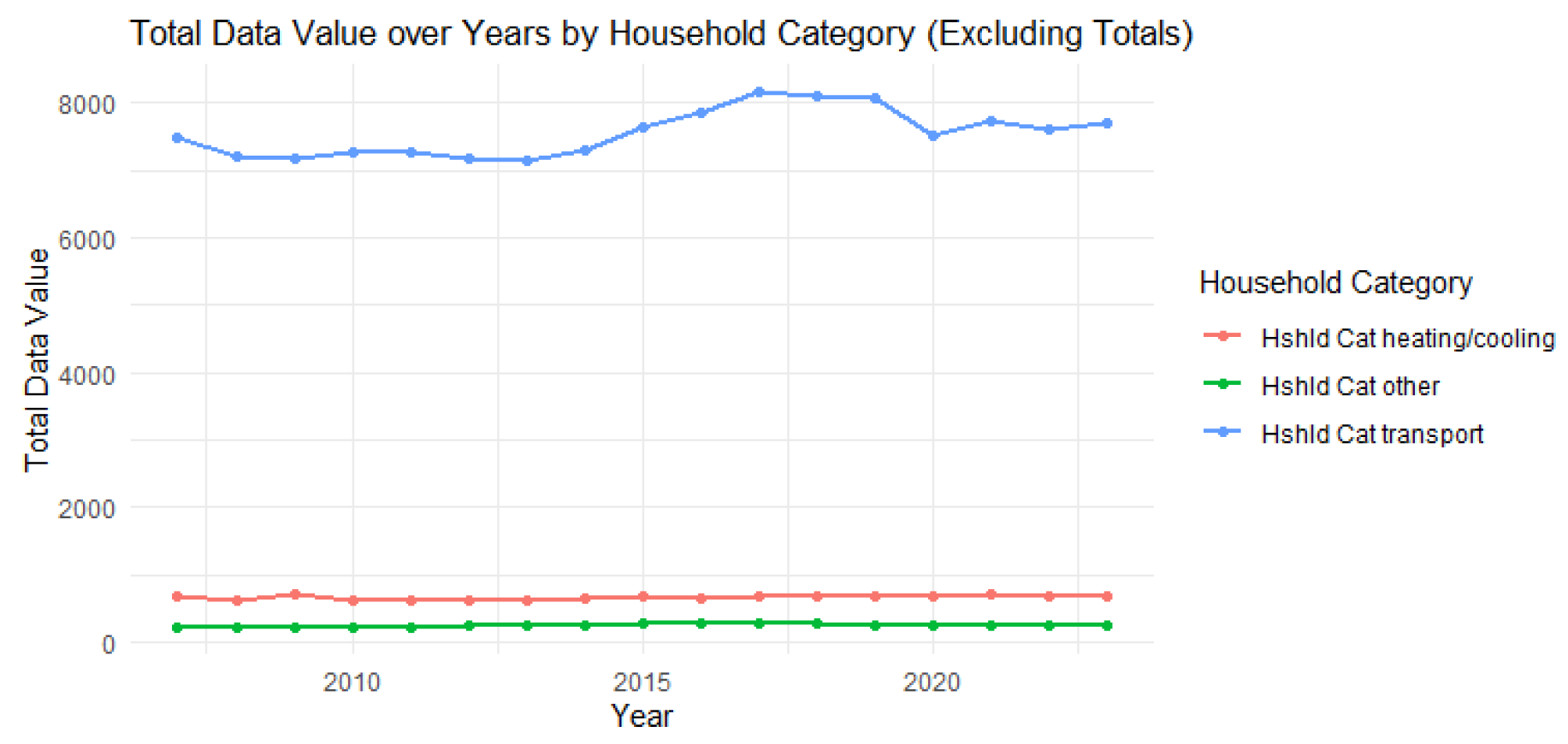
The figure depicts the trends in total data values for various household categories over a series of years. Each line on the graph denotes a specific household category, with Household Category heating/cooling depicted in red, Household Category other in green, and Household Category transport in blue, as specified in the legend on the right.

The data value for each category is represented on the y-axis, while the x-axis represents the affected countries in a specific period. This makes it easier to see the changes over time. The blue line represents the category of Household Category transport which is much higher than the other categories. This demonstrates that in the case of transportation, other categories are either never fully utilized or are less utilized if they are employed at all. The transport category does not show much variation from year to year and peaked between 2015 and 2016, only to drop and later settle significantly less in subsequent years.

On the other hand, the red (Hshld Cat heating/cooling) and green (Hshld Cat other) lines remain relatively stable around low values which implies that there is little change and it has a relatively low effect on the data value. This graph demonstrates the dominance of the transport category within total data values of carbon emissions over the years while heating/cooling and other categories do not provide much input and show low change in carbon emissions over the years.

2.5.c. Regional Disparities in Emissions

The subset() function filters the dataset to include only records where the year is between 2007 and 2022, ensuring we analyze data for this period. To calculate the mean Data_value for each region we use aggregate() to calculate the mean ‘Data_value’ for each unique ‘Region’ in the filtered dataset. The result is stored in a new data frame, ‘mean_data’, with two columns: ‘Region’ and ‘Data_value’ (mean).

The function ggplot() initializes the plot with ‘mean_data’ as the data source. The aes() defines ‘Region’ (sorted by decreasing mean Data_value) on the x-axis and the mean ‘Data_value’ on the y-axis. The geom_bar(stat = “identity”) creates a bar for each region, with bar height corresponding to the mean Data_value. The fill = “skyblue” sets the bar color to sky blue. The labs() function provides labels for the plot’s title, x-axis, and y-axis. Using theme_minimal() applies a minimalistic theme to the plot and theme(axis.text.x = element_text(angle = 45, hjust = 1)) rotates x-axis labels for readability.

Figure 3. Bar Chart of Regional Mean of Carbon Emissions.

Figure 3. Bar Chart of Regional Mean of Carbon Emissions.

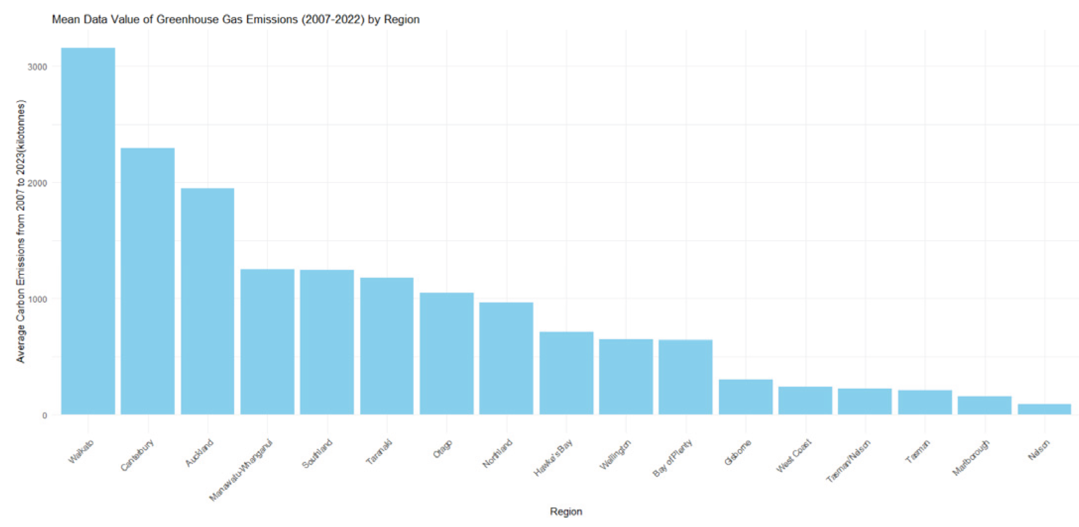
The bar graph above, titled “Mean Data Value of Greenhouse Gas Emissions (2007-2022) by Region,” illustrates the 17 regions of Australia and New Zealand where the levels of greenhouse gas emissions were documented across different industries within those areas. To determine the typical level of greenhouse gas emissions from every region. The total greenhouse gas emissions for each year from 2007 to 2022 were collected and then the average was calculated. The y-axis represents the “Average Carbon Emission in Kilotonnes,” whereas the x-axis denotes the different “Regions” in Australia and New Zealand.

In this instance, we observe that Waikato possesses the highest average emissions throughout this timeframe, exceeding 3000 kilotons. Canterbury and Auckland come next, both having emissions that average more than 2000 kilotonnes. Areas like Manawatū-Whanganui, Southland, Taranaki, and Otago exhibit moderate emission amounts, falling within the range of 1000 to 1500 kilotonnes. Northland and Hawke’s Bay exhibit average emissions that are lower, ranging from 700 to 1000 kilotonnes. Wellington and Bay of Plenty exhibit even smaller averages, roughly 500 to 700 kilotonnes. Gisborne, West Coast, Tasman/Nelson, Marlborough, and Nelson exhibit the lowest average emissions, with Nelson ranking the lowest, under 200 kilotonnes. Waikato, Canterbury, and Auckland are the primary sources of greenhouse gas emissions, suggesting they might have elevated industrial activities, populations, or energy requirements relative to other areas. Areas with smaller economies or lower industrialization, like Nelson and Marlborough, display reduced emissions.

2.6. Conclusion of EDA

The examination and representation of greenhouse gas emissions among different industries and regions offer a detailed overview of present emissions and highlight vital areas for enhancement. The emissions by sector pie chart distinctly shows that agriculture is the primary contributor, representing 18.6% of total emissions.

Emissions scenario is made further complicated due to regional disparities. The regional bar chart showing emissions indicates that regions like Waikato, Canterbury and Auckland, which are highly industrialized, have the highest average emissions, suggesting these high emission regions may be causing emissions due to energy-intensive industries coupled with high demand from the people of the area. Conversely, more industrialized areas, such as Nelson and Gisborne, are associated with lower levels of emissions. The problem of this situation clearly demonstrates the need for regional policies which, on the one hand, enhance energy efficiency in the high emission regions but at the same time promote regional development in low emission regions.

At last, the data indicates the need for a viewing emission reduction from more than one perspective. This should be able to address the unique requirements of different sectors such as curtailing emissions from agriculture, residential and manufacturing sectors using cleaner energy, and developing urban transport systems in environmentally friendly ways.

3.0. Methods

3.1. Statistical Data Analysis Methods

In this paper, many statistical data analysis methods [22,23,24] were used to verify previous papers and obtain insights on the dataset. These include descriptive statistics, data transformation (feature engineering), frequency counts, data filtering and aggregation, and data visualization[25,26,27,28]. The details of these methodologies are shown in the following table.

Table 3. Explanation of data analysis methodologies.

Table 3. Explanation of data analysis methodologies.

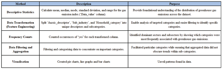3.2. Appropriate Data Analysis

The methodologies provided in the table were suitable for this data analysis paper as they facilitated a comprehensive examination of greenhouse gas emissions. By converting categorical data into multiple binary columns, we conducted frequency analysis on each category, yielding a profound comprehension of emissions by sector and category. Descriptive statistics provide a summary of the data distribution, whereas visualisation methods effectively illustrate trends and discrepancies. These methodologies correspond with the research purpose of analysing emission patterns temporally and categorically.

3.3. Descriptive Statistics for ‘Data_Value’

Descriptive statistics were used for the Data_value column to comprehend the greenhouse gas emissions in the dataset. The statistical calculations include the mean, median, mode, standard deviation, and range. The median mitigated the outliers, whereas the mean showed the average emissions. The mode represents the most often occurring emission value. The variability and dispersion of emissions data were evaluated using the standard deviation[30,31,32]. The structured string (“min - max”) range disclosed dataset emission values. The descriptive statistics facilitated a preliminary quantitative evaluation of the emissions distribution, distinguishing between normal and abnormal emission values for subsequent analysis.

3.4. Transformation for Categorical Analysis

The ‘Anzsic_descriptor’, ‘Sub_industry’, and ‘Household_category’ columns were transformed from a categorical string format into binary columns, representing data values of “yes” or “no” for categorical analysis. A binary column was assigned to each distinct descriptor, indicating its presence. This enabled thorough filtering and analysis of emissions linked to specific industries, sub-industries, and household categories. The “All” items in the ‘Sub_industry’ and ‘Household_category’ underwent additional processing, specifically for marking “yes” for records with “yes” across all sub-grouping columns.

3.5. Frequency Counts and Visualisation

This research employed categorical transformation to allow accurate filtering and analysis, which made it possible to isolate greenhouse gas emissions associated with particular industries, sub-industries, and household types. This approach facilitated efficient categorical analysis and revealed important patterns and trends.

Frequency counts enable the visualisation of textual data. The utilisation of visualisations – including pie charts, line graphs, and bar plots – improved data interpretation and highlighted sectors and categories with the highest and lowest impact on greenhouse gas emissions.

3.6. Conclusion of Data Analysis

The integration of descriptive statistics, data transformation, frequency counts, and visualizations created a comprehensive analytical framework. Every approach offered unique perspectives, from understanding general emission patterns to identifying particular categories and sectors that contribute the most to greenhouse gas emissions. Together, these methods facilitated an exhaustive examination of greenhouse gas emissions data, fulfilling the research objectives and highlighting clear relationships among categories, emissions trends, and time-related patterns.

4.0. Results and Discussion

This chapter includes the results of the research work dealing with greenhouse gas emissions per sector and region using both exploratory data analysis (EDA) techniques and statistical methods.

4.1. Result of Exploratory Data Analysis

The exploratory data analysis uncovered substantial trends in greenhouse gas emissions across sectors and regions. The main findings are as follows:

4.1.a. Sectoral Emissions

Agriculture was identified as the primary contributor to greenhouse gas emissions, representing 18.6% of the overall total. Farming methods like raising livestock, utilizing fertilizers, and clearing forests greatly enhance methane and CO₂ emissions.

Additional major contributors are households (3.6%), transportation (2.1%), and manufacturing (2.3%). Household emissions were primarily linked to energy consumption, including heating, cooling, and electricity consumption, while emissions from the services sector were indicative of activities in public services and companies not related to transportation.

Sectors which transported citizens (0.6%) do not include other industries such as mining (0.3%), construction (0.3%), government (0.2%), defence (0.2%), education (0.2%),

health care (0.2%), wholesale (0.2%), retail trade (0.2%), accommodation (0.2%) and many other sections that have relatively small contributions to the economy.

4.1.b. Urban Transportation Emissions

Increased urbanization alongside the growth of fossil-fuel reliant vehicles may have accounted for the transport emissions being one of the highest sources of greenhouse gas emissions in the world. In areas that are well urbanized, transportation was one of the main greenhouse gases emitted globally. Emission rates stabilised to lower levels 6 years after 2015, which signifies a progressively low dependency on vehicles.

When compared to transportation, other household emissions worsen but at a much more gradual rate which can be viewed in the trends. The data is put forth in a manner that makes it seem like the reduction of greenhouse gas emissions from vehicles in urban settings, would also mean the use of electric cars or increased public transit efficiently worked.

4.1.c. Regional Emission Disparities

A large amount of variation can be seen in the emission levels that several regions possess, it is no surprise, some record extremely high average emissions while others struggle. Waikato, Canterbury, and Auckland all gained the most average emissions during this time.

The elevated emissions in Waikato are probably due to agricultural and industrial activities, while Auckland’s emissions stem from its large population, urban development, and related transportation requirements. Emissions in Canterbury may arise from both farming practices and industrial activities.

Areas with reduced emissions, like Nelson and Gisborne, have smaller populations and less industrial activity, which likely explains their smaller carbon footprint. These results emphasize the necessity for region-specific policies, since emissions trends are closely linked to local industrial activities, population density, and infrastructure.

4.2. Result of Statistical Method

The statistical research employed various methods to evaluate and analyze greenhouse gas emissions data, leading to a deeper, more accurate comprehension of emissions across different industries and areas. This part emphasizes the techniques employed and the knowledge acquired from them.

4.2.a. Descriptive Statistics

Preliminary analysis subjected descriptive measures, such as mean, median, mode standard deviation, and range, to each region and each sector. Means and medians reinforced essential patterns as they signposted general emissions in different sectors and regions. The results revealed that agriculture emitted on average more emissions than the other sectors in line with the findings of the EDA.

The standard deviation revealed the extent to which emission levels differed across sectors and between sectors with agriculture and manufacturing having the highest. Such differences illustrate that within the same category, some agricultural and industrial practices are much more emission intensive than others. The emission range, which indicated the difference between the highest and lowest emission levels, helped in pinpointing outliers and assessing whether particular sectors exhibited notably high emissions that needed more investigation.

4.2.b. Frequency Counts

To identify the sub-sectors most frequently linked to high emissions, frequency counts were utilized on categorical information like ANZSIC descriptors, sub-industries, and types of households. Agriculture and households exhibited the highest frequency counts, reinforcing their important role as sources of emissions.By focussing on frequently occurring categories, our research helped identify areas where interventions could be most beneficial. For example, focussing emissions reduction efforts on the agricultural sub-industries with the greatest counts (such as cattle farming) could result in large improvements.

4.2.c. Categorical Transformations

In order to aid analysis, categorical transformations were carried out to some set of categories to allow for filtering and analysis in the binary format of 1 and 0. This approach permitted the research to seek important sub-groups within larger groups and more easily control for other aspects, such as emissions from different crops. This approach allowed for more finely grained information on where emissions come from by looking at single activities in each sector. For example, the emissions from agriculture were less informative than emissions from livestock in agriculture on its own.

4.2.d. Techniques for Visualisation

To represent emissions data in clear and accessible formats, several visualization methods were employed, such as pie charts, line graphs, and bar charts. These visualisations were critical in explaining the EDA and statistical analysis results.

The pie graphic demonstrated that agriculture is the largest contributor to emissions, emphasising the importance of prioritising interventions in this sector. The line graph showed persistent emissions from urban mobility, emphasising the importance of transport on greenhouse gases and the necessity for sustainable alternatives in cities. The regional emissions bar chart allowed for direct comparisons between areas, with Waikato, Canterbury, and Auckland coming out on top.

The statistical analysis thus supplements the EDA findings by offering a structured approach to analysing and quantifying greenhouse gas emissions.Through the use of descriptive and inferential statistical methods, the study confirmed the primacy of agricultural and transportation activities in emissions, signalled regional disparities, and drew theoretically relevant conclusions. These results are good for the analyses aimed at developing specific policies to reduce emissions in both large and small industries as well as in particular areas with high emission indices.

4.3. Interpretation of Results

The two main methods used to understand this piece of data are descriptive statistics and data visualisation. In this section, both methods are used to get a deeper analysis of the greenhouse gas emission in Australia and New Zealand.

4.3.a. Sectoral Emissions

It is shown in the exploratory data analysis that the most predominant source of emissions was the agriculture industry with livestock production, fertiliser use and deforestation being the main contributing factors. This is supported by the results of the descriptive statistics which indicate that the agriculture industry has a relatively high mean amount of emissions and has a high standard deviation as well which shows a significant variability of the agriculture sector. This high variability suggests that certain practices within the agriculture industry are responsible for much higher emissions than others. Efficient reduction of emission from agriculture, could be achieved by focusing on specific high emission practices.

4.3.b. Urban Transportation Emissions

The chart titled “Total Data Value over Years by Household Category (Excluding Totals) shows a steady and relatively high source of carbon emissions from transportation in the household category. This means efforts to reduce carbon emissions could be effective if focused in urban areas.

4.3.c. Regional Emissions Disparities

According to the barchart in the EDA titled “Mean Data value of Greenhouse Gas Emissions (2007-2022) by Region” a significant difference in regional emissions were found. Waikato, Canterbury, and Aukland showing the highest levels (Waikato being the highest). These high emissions are understandable for the region as the main industry in Waikato is agriculture (Keenan, Mackay, & Paragahawewa, 2023, p. 5).

4.4. Result Comparison

This section notes the comparison of results amongst sectors, regions and statistical methodologies to show the similarities, differences, and highlights of greenhouse gas emissions in New Zealand.

Agriculture, as the largest contributor of greenhouse gases (18.6%), is far higher than than the second largest contributor of greenhouse gases; that is the household category (10.3). This large difference shows that focusing our efforts on agricultural emissions is paramount to achieving significant reductions in overall greenhouse gas emissions.

The sustained contribution of urban transport (2.1%) to total emissions mirrors findings in countries with similar urbanisation rates. However, the peak between 2015 and 2016 and subsequent stabilisation at lower levels may reflect the impact of incremental policy measures, such as vehicle fuel standards (Stratas Advisors, 2015) or early electric vehicle adoption initiatives (Broadbent, Metternicht, Wiedmann, and Allen, 2024, p. 3).

Regional breakdowns put Waikato, Canterbury, and Auckland as the top three emitters of greenhouse gas, reflecting their population density, industrial activity, and agricultural practices. Waikato comes out as an agriculture-driven case-a common trend globally in rural regions-whereas transportation and energy use dominate the urban emissions of Auckland. These findings support existing studies that urban centres and agricultural areas are usually the highest emitters of greenhouse gases. Regions like Nelson and Gisborne, with much smaller populations and less industrial activity, would then be responsible for less greenhouse emissions. That would mean opportunities for growth in these regions without extreme increases in emissions-a trend seen in countries prioritising green development in low-emission areas (Greenhouse Gases down in Most New Zealand Regions in 2023 | Stats NZ, 2023).

5.0. Limitation and Future Study

This section outlines the core findings of the study, focusing on emission trends across industries, households, and regions in New Zealand. Using statistical measures, such as the mean and median, the analysis highlights key patterns and variability in emissions, providing a holistic view of their distribution and contributing factors.

5.1. Major Findings

This study assesses the greenhouse gas emissions of New Zealand between 2007 and 2022 by household class, industry, and region. A method for assessing emissions was developed by binary encoding specific industry and household activities. Statistical calculations mean, median, modal, standard deviation, and range were used to extract central information on trends in emissions. Here, the median mitigated the effect of outliers, while the mean emphasized average emission levels. The standard deviation assesses how much the emission values differ, and the mode is used to find emission values that occurred most frequently. Together with the methods used, standalone to give a holistic view of emissions trends showing variation and pattern among different household types and sectors.

5.2. Results Interpretation with Respect to Outside Sources

According to further research done by the New Zealand Ministry for the Environment and Statistics NZ, the results confirm that sectors such as forestry, fisheries, agriculture, and energy generation rank among the top emitters of greenhouse gases. Greenhouse gases from households put forward earlier research that identifies them as substantial contributors, especially from transportation and heating or cooling. By focusing on trends and differences across categories, trend graphs and categorical bar plots, within the data visualisation family, supplemented the very analysis. Those figures provide a coherent story in compliance with the global climatic gas emission reporting standards. (noted in 3.5)

5.3. Identified Limitations

5.3.a. Redundancy in Binary Encoding

This involves the higher dimensionality level in the dataset as categorical data is turned into binary columns. Take `Anzsic_descriptor` for instance, where each of its categories takes up a new binary column. This could result in redundancy, leaving the analysis more complex for computation purposes. (as seen in 3.3.b)

Normalized, categorical features such as Sub_industry and Household_category were binary encoded, leading to a large jump in column numbers and high-dimensional data. This additional information could lead to multicollinearity problems, which could make interpretation difficult and also have an impact on the performance of statistical models in other contexts.

5.3.b. Impact of Outliers

The median would do its job of minimizing outliers but could still influence other calculations in others such as the mean or the standard deviation from the extreme values reported in particular sectors over certain years, which were described as emission spikes (as seen in 4.3). The means were protected from the outliers after assigning the latter to their respective lower positions of data distribution. However, the effects from any outlier have the potential to undermine the relative influence of certain computations. A spike in one company’s greenhouse gas emissions could, for example, raise the mean and increase the range, possibly skewing the general interpretation of the trends. (as seen in 4.3)

5.3.c. Visualisation Complexity

The very high dimensionality of the binary-encoded data also renders it practically impossible to visualize effectively. Plots and charts were provided to show key trends; however, the fact that data were presented over 7,000 rows and varied categories required dramatic simplifications that might have lost some nuances of significance (as seen in 3.5). The sheer size of the dataset made visualisation very difficult. Even with basic visualisations like bar and line graphs, it is tedious to visualise emission patterns across several businesses and household groups which might bury some important facts. (as seen in 3.5)

5.3.d. Granularity of Data and Lack of Consistency over Years

Without a clear delineation of these broad categories such as “Forestry and Logging” or “Heating/Cooling”, it is very challenging to identify specific emissions drivers in this tier. The study is limited by the categories into which it groups activities from the industry and household sectors, precluding the identification of drivers of emissions. For instance, “Transport” records emissions produced by private and public means of transport, this prevents the dataset from generating useful information.

Intermittencies of the data for various years for certain industries and household activities sprung doubt and negated the use of robust time-series analyses to explain or identify patterns over time. Weaker time series analyses, with a number of sections failing to include data from certain years. In addition, this limitation also made trying to model accurate emissions’ patterns during the study period more difficult.

5.3.e. Narrow Focus on Emissions Without Contextual Factors

Treating emissions on their own without an appreciation of their influencing factors – the dataset fails to solicit any information concerning technological progress, economic development, or policy intervention all of which are key to understanding the great context of emissions trends.

5.4. Proposed Future Directions

Based on the limitations established, this section discourses some solutions as well as future research tendencies. Advanced statistical methods, better visualization tools, and adding more contextual variables to deepen and broaden emissions analysis all fall into this category.

5.4.a. Enhanced Statistical Techniques

As a remedy to the drawbacks of binary encodings, which was also done in order to deal with outlier values, more advanced statistical approaches should be considered in additional research. For instance, outliers in mean and range computations can alternatively be managed using robust statistical techniques and redundancy can be mitigated using dimensionality reduction techniques like Principal Component Analysis.

5.4.b. Incorporating Binary Encoding for Categorical Analysis

The study emphasizes the importance of the use of binary encoding for categorical analysis within the scope of effective emissions filtering and comparison with individual companies and households. The strategy could be enhanced in future studies to incorporate automated feature selection techniques in order to retrieve only those features which bear relevance with minimum redundancy.

6.3.c. Improved Data Visualization

Modern visualization technologies, including interactive dashboards, could visualize complicated high-dimensional datasets. The advanced technologies allow for exploration and interrogation of patterns within regions and sectors, improving usability and understanding.

6.3.d. Additional Contextual Variables and Data Imputation

Future studies should incorporate socio-economic factors, such as domestic and foreign credit, regulatory changes, and technological changes to provide context for the emissions data. Those factors would thus provide a broader understanding of the reasons for emission trends. Imputation approaches include regression or machine learning techniques to fill in the gaps in the datasets and thus improve time series analysis reliability.

6.3.e. Binary Encoding Optimization and Improvement of Statistical Analysis

The prospective studies are suggested to investigate low-frequency categories in `Sub_industry` and `Household_category` into the column called “Other,” thus enabling decreased dimensionality without sacrificing the analytical depth. Apart from this, categorical variables could efficiently be represented through dense vectors, such as categorical embeddings, widely used in machine learning, reflecting correlations among various categories with analytical advantages. This approach, together with variability measures, for example interquartile ranges, can help in the understanding of data trends and data dispersion through the mean, median and standard deviation.

6.3.g. Holistic Learning with a Focus on Impact on Renewable Energy

Still, omitted from the dataset is renewable energy use, and future research should investigate how this may reduce emissions, they write. These future studies would obtain a more comprehensive view of the emissions dynamics and mitigation strategies.

6.3.h. Global Comparisons

Global data can provide a comparative perspective on emissions behaviors, enabling better understanding and decision-making to prevent climate change disasters in New Zealand and worldwide.

6.0. Conclusion

In conclusion, this study provides a comprehensive analysis of New Zealand’s GHG emissions which allows us to gain valuable insights especially for policy makers and stakeholders. The study highlights sector-specific measures and regional disparities for the youth to achieve a greener future, recommending future research on international comparisons and renewable energy impacts.

References

- Alchemer. What is Regression Analysis and Why Should I Use It? | SurveyGizmo Blog; Alchemer, 8 June 2021. https://www.alchemer.com/resources/blog/regression-analysis/.
- Faheem, H.B.; Shorbagy, A.M.E.; Gabr, M.E. Impact Of Traffic Congestion on Transportation System: Challenges and Remediations - A review. Mansoura Engineering Journal 2024, 49. [Google Scholar] [CrossRef]
- Gössling, S.; Neger, C.; Steiger, R.; Bell, R. Weather, climate change, and transport: a review. Weather, Climate Change, and Transport 2023, 118, 1341–1360. [Google Scholar] [CrossRef]
- Greenhouse gases down in most New Zealand regions in 2023 | Stats NZ. (2023). Govt.nz. https://www.stats.govt.nz/news/greenhouse-gases-down-in-most-new-zealand-regions-in-2023/.
- Infometrics. (n.d.). Regional Economic Profile | New Zealand | Economy structure. Rep.infometrics.co.nz. Retrieved November 15, 2024, from. https://rep.infometrics.co.nz/new-zealand/economy/structure. Industry structure of economy | Focus Year: 2023.
- Leahy, S.; Journeaus, P.; Kearney, L. Greenhouse gas emissions on New Zealand farms: a companion guide to the climate change seminars for rural professionals. New Zealand Agricultural Greenhouse Gas Research Centre. https://www.nzagrc.org.nz/publications/rural-professionals-seminar-booklet/?gad_sou rce=1&gbraid=0AAAAAozA4P8s9mVWtDvf5WwFvCU8uR6T0&gclid=Cj0KCQiA ire5BhCNARIsAM53K1hryt2V5w3140aS1WmitInyvdAoCA7NRYvDdoT9a5Uo7rZ 9ovHorYYaAjb1EALw_wcB. 2021.
- Ministry for the Environment. (2024, April 18). New Zealand’s Greenhouse Gas Inventory 1990–2022: Snapshot. Ministry for the Environment. https://environment.govt.nz/publications/new-zealands-greenhouse-gas-inventory-199 02022-snapshot/ Ministry of Business, Innovation & Employment. (2016). New Zealand energy sector greenhouse gas emissions | Ministry of Business, Innovation & Employment. Govt.nz. https://www.mbie.govt.nz/building-and-energy/energy-and-natural-resources/energy-s tatistics-and-modelling/energy-statistics/new-zealand-energy-sector-greenhouse-gas-e missions.
- National Grid. (2023, February 23). What are greenhouse gases? | National Grid Group. Www.nationalgrid.com; National Grid. https://www.nationalgrid.com/stories/energy-explained/what-are-greenhouse-gases.
- Nguyen, T.T.; Grote, U.; Neubacher, F.; Rahut, D.B.; Do, M.H.; Paudel, G.P. Security risks from climate change and environmental degradation: implications for sustainable land use transformation in the Global South. Current Opinion in Environmental Sustainability 2023, 63, 101322. [Google Scholar] [CrossRef]
- Nunez, C. Carbon dioxide in the atmosphere is at a record high. Here’s what you need to know. National Geographic. 13 May 2019. https://www.nationalgeographic.com/environment/article/greenhouse-gases.
- Rewiring Aotearoa. ContentKeeper Content Filtering. Rewiring.nz. 2024. https://www.rewiring.nz/electrification-guides/space-heating-and-cooling.
- Ritchie, H. Sector by sector: where do global greenhouse gas emissions come from? Our World in Data. 2020. https://ourworldindata.org/ghg-emissions-by-sector.
- Shivanna, K. R. Climate Change and Its Impact on Biodiversity and Human Welfare. Proceedings of the Indian National Science Academy 2022, 88, 160–171. [Google Scholar] [CrossRef]
- Stats, NZ. Greenhouse gas emissions (industry and household): Year ended 2021 | Stats NZ. Www.stats.govt.nz. 31 May 2023. https://www.stats.govt.nz/information-releases/greenhouse-gas-emissionsindustry-an d-household-year-ended-2021/.
- Stats, NZ. Quarterly greenhouse gas emissions (industry and household): Sources and Methods - Stats NZ DataInfo+. Govt.nz. 28 August 2024. https://datainfoplus.stats.govt.nz/item/int.example/ae681659-d7fc-40dc-a8c7-4e2b379 7668e.
- Tableau. Time Series Analysis: Definition, Types, Techniques, and When It’s Used. Tableau. 2024. https://www.tableau.com/analytics/what-is-time-series-analysis.
- Tātai Aho Rau Learnz. Primary Industries in New Zealand | LEARNZ. Learnz.org.nz. 2016. https://www.learnz.org.nz/primaryindustries172/bg-standard-f/primary-industries-in-n ew-zealand.
- United States Environmental Protection Agency. Climate Impacts on Agriculture and Food Supply | Climate Change Impacts | US EPA. Climatechange.chicago.gov; United States Environmental Protection Agency. 2020. https://climatechange.chicago.gov/climate-impacts/climate-impacts-agriculture-and-fo od-supply.
- USGS. How can climate change affect natural disasters? | U.S. Geological Survey. Www.usgs.gov; U.S. Geological Survey. 2023. https://www.usgs.gov/faqs/how-can-climate-change-affect-natural-disasters.
- Yang, Z.; Kagawa, S.; Li, J. Do greenhouse gas emissions drive extreme weather conditions at the city level in China? Evidence from spatial effects analysis. Urban Climate 2021, 37, 100812. [Google Scholar] [CrossRef]
- Khandelwal, M.; Rout, R.K.; Umer, S.; Sahoo, K.S.; Jhanjhi, N.Z.; Shorfuzzaman, M.; Masud, M. (. A Pattern Classification Model for Vowel Data Using Fuzzy Nearest Neighbor. Intelligent Automation & Soft Computing 2023, 35. [Google Scholar]
- Sindiramutty, S.R.; Prabagaran, K.R.V.; Jhanjhi, N.Z.; Murugesan, R.K.; Malik, N.A.; Hussain, M. Ethics and Transparency in Secure Web Model Generation. In Reshaping CyberSecurity With Generative AI Techniques; IGI Global, 2025; pp. 411–464. [Google Scholar]
- JingXuan, C.; Tayyab, M.; Muzammal, S.M.; Jhanjhi, N.Z.; Ray, S.K.; Ashfaq, F. Integrating AI with Robotic Process Automation (RPA): Advancing Intelligent Automation Systems. 2024 IEEE 29th Asia Pacific Conference on Communications (APCC), 2024, November; IEEE; pp. 259–265. [Google Scholar]
- Al-Quayed, F.; Javed, D.; Jhanjhi, N.Z.; Humayun, M.; Alnusairi, T.S. A hybrid transformer-based model for optimizing fake news detection. IEEE Access 2024, 12, 160822–160834. [Google Scholar] [CrossRef]
- Mushtaq, M.; Ullah, A.; Ashraf, H.; Jhanjhi, N.Z.; Masud, M.; Alqhatani, A.; Alnfiai, M.M. Anonymity assurance using efficient pseudonym consumption in internet of vehicles. Sensors 2023, 23, 5217. [Google Scholar] [CrossRef] [PubMed]
- Gouda, W.; Sama, N.U.; Al-Waakid, G.; Humayun, M.; Jhanjhi, N.Z. Detection of skin cancer based on skin lesion images using deep learning. Healthcare 10, 1183. [CrossRef] [PubMed]
- Barral, D.; Cardama, F.J.; Diaz-Camacho, G.; Faílde, D.; Llovo, I.F.; Mussa-Juane, M.; … Gómez, A. Review of distributed quantum computing: from single QPU to high performance quantum computing. Computer Science Review 2025, 57, 100747. [Google Scholar] [CrossRef]
- Tennie, F.; Laizet, S.; Lloyd, S.; Magri, L. Quantum computing for nonlinear differential equations and turbulence. Nature Reviews Physics 2025, 7, 220–230. [Google Scholar] [CrossRef]
- Fajinmi, J.; Oloyede, J. State-of-the-Art Robotic Technologies in Fighting the COVID-19 Pandemic. 2025. [Google Scholar]
- Javed, D.; Jhanjhi, N.Z.; Ashfaq, F.; Khan, N.A.; Das, S.R.; Singh, S. Student Performance Analysis to Identify the Students at Risk of Failure. 2024 International Conference on Emerging Trends in Networks and Computer Communications (ETNCC), 2024, July; IEEE; pp. 1–6. [Google Scholar]
- Saeed, S.; Jhanjhi, N.Z.; Abdullah, A.; Naqvi, M. (. Current Trends and Issues Legacy Application of the Serverless Architecture. International Journal of Computing Network Technology 2018, 6. [Google Scholar] [CrossRef]
- Humayun, M.; Sujatha, R.; Almuayqil, S.N.; Jhanjhi, N.Z. A transfer learning approach with a convolutional neural network for the classification of lung carcinoma. Healthcare 2022, 10, 1058. [Google Scholar] [CrossRef] [PubMed]
Disclaimer/Publisher’s Note: The statements, opinions and data contained in all publications are solely those of the individual author(s) and contributor(s) and not of MDPI and/or the editor(s). MDPI and/or the editor(s) disclaim responsibility for any injury to people or property resulting from any ideas, methods, instructions or products referred to in the content. |
© 2025 by the authors. Licensee MDPI, Basel, Switzerland. This article is an open access article distributed under the terms and conditions of the Creative Commons Attribution (CC BY) license (http://creativecommons.org/licenses/by/4.0/).
Copyright: This open access article is published under a Creative Commons CC BY 4.0 license, which permit the free download, distribution, and reuse, provided that the author and preprint are cited in any reuse.