
Submitted:
02 December 2025
Posted:
03 December 2025
You are already at the latest version
Abstract
Accurate crop yield information is crucial for regional agricultural monitoring; however, many existing approaches rely on complex models or extensive input datasets. This study presents a low-complexity method for estimating county-level maize and sunflower yields in Fejér County, Hungary, using Harmonized Landsat–Sentinel (HLS) Normalized Difference Vegetation Index (NDVI) time series at 30 m spatial resolution. Seasonal NDVI profiles were smoothed using a double-Gaussian fitting approach. Two modelling strategies were investigated: a robust approach using all agricultural pixels and a crop-specific approach restricted to maize or sunflower pixels. The models were tested through leave-one-year-out cross-validation against official yield statistics. For maize, the crop-specific predictive model provided the most accurate estimates (R² = 0.997; mean absolute percentage error (MAPE) = 2.0%). The MAPE remained below 4% even about 30–50 days before the end of harvest. For sunflower, the highest accuracy was obtained using the robust predictive model (R² = 0.928; MAPE = 2.73%). All models showed stable performance across years, including the extreme drought year of 2022. These findings indicate that a simple NDVI-based method can provide reliable county-scale yield estimates and may serve as a practical component in regional monitoring or early-warning systems.
Keywords:
NDVI time-series
; Harmonized Landsat–Sentinel
; County-scale yield prediction
; maize
; sunflower
1. Introduction
As the world population increases and environmental stresses intensify, the reliable prediction of crop production has become both an economic necessity and a strategic priority [1,2]. Timely and accurate crop yield estimation at global, national, and regional scales is essential for modern agricultural management, ensuring global food security, balancing international grain trade, and promoting sustainable agricultural development [3,4,5].
The application of remote sensing technologies in agriculture began with the launch of the Landsat satellite, equipped with the Multispectral Scanner (MSS) in 1972 [6]. Since then, remote sensing has become a widely used technique in agriculture [7] and has played a significant role in assessing crop production over the years [8]. Satellite-based remote sensing technology has rapidly developed into a widely applied tool for crop yield estimation [9,10]. For large-scale yield monitoring, it is necessary that remotely sensed data be available reliably and consistently over several years, and that the temporal resolution of the data be sufficiently dense. The combination of high temporal frequency, wide spatial coverage, and low cost makes remote sensing an ideal choice for national- and regional-level crop yield estimation applications [11].
In previous decades, this requirement was met, for example, by data from the AVHRR (Advanced Very High Resolution Radiometer, ~1 km spatial resolution) instrument aboard the NOAA (National Oceanic and Atmospheric Administration) satellites, or from the MODIS (Moderate Resolution Imaging Spectroradiometer, 250–500 m spatial resolution) sensors on the Terra and Aqua satellites. With the advent of the new-generation multispectral Sentinel-2 satellite constellation (Sentinel-2A, launched in 2015; Sentinel-2B, launched in 2017; and Sentinel-2C, launched in 2024) by the European Space Agency new opportunities have emerged for long-term, frequent monitoring of agricultural landscapes [12]. The Multispectral Imager (MSI) onboard all three satellites provides high-resolution optical observations in 13 spectral bands with a spatial resolution between 10 m and 60 m, and a revisit frequency of 2–5 days when two satellites are operational [13]. Around the same time, in 2013, the National Aeronautics and Space Administration (NASA) launched Landsat-8, the new member of the more than 40-year-old Landsat series [14], followed by Landsat-9 in 2021 [15]. Both satellites carry the Operational Land Imager (OLI) instrument, with a spatial resolution of 30 m (15 m for panchromatic) and a revisit time of 16 days [16]. Landsat-9 has the important mission of working together with Landsat-8 to reduce the revisit period of Landsat Earth observations to eight days [17].
It has been well established that combining data from different satellite sensors provides greater opportunities for cloud-free surface observation [18,19,20]. Given that Landsat-OLI and Sentinel-MSI make similar measurements in terms of spectral, spatial, and angular characteristics [12,21], it was a natural step to integrate data from the two instruments into a unified system. This project, known as the Harmonized Landsat/Sentinel-2 (HLS), provides high-frequency global imagery products (excluding Antarctica) with a spatial resolution of 30 m every two to three days since the launch of Landsat-9 [22]. Such dense and consistent data are critical for various applications, including continuous crop monitoring and yield estimation [23].
Remote sensing–based yield estimation models are generally categorized into three main types: data assimilation models, light-use efficiency models, and empirical statistical models [24]. Empirical statistical models do not require numerous input parameters [25]; therefore, their use is widespread due to their relative simplicity, rapidity, and computational ease [26,27]. In recent years, these conventional models have produced remarkable results in yield estimation [28,29]. Such models mainly rely on linear relationships between crop yield and characteristic spectral bands or vegetation indices , sometimes supplemented by basic meteorological or agronomic data [30,31,32,33,34,35]. Here, observations from the past are used to inform what is happening in the present, without a strong need for understanding of the causality [36]. In these studies, the most commonly used vegetation index is the Normalized Difference Vegetation Index (NDVI) [37,38], which is strongly correlated with photosynthetic capacity, and thus yield [36].
Building on a previously developed robust yield estimation method based on a regression method, which has been successfully applied to several crop species [39,40], the present study aims to further refine and extend this approach using a simple empirical regression yield estimation method for maize and sunflower based on HLS NDVI data. To achieve this, we addressed the following main goals: (i) improve the previously developed robust method based on 30-m data, (ii) test the model on input data from areas with different vegetation cover, (iii) estimate the predictive power of the model, and (iv) test the accuracy of the model for forecasts at different dates.
2. Materials and Methods
2.1. Study Area and Crop Information
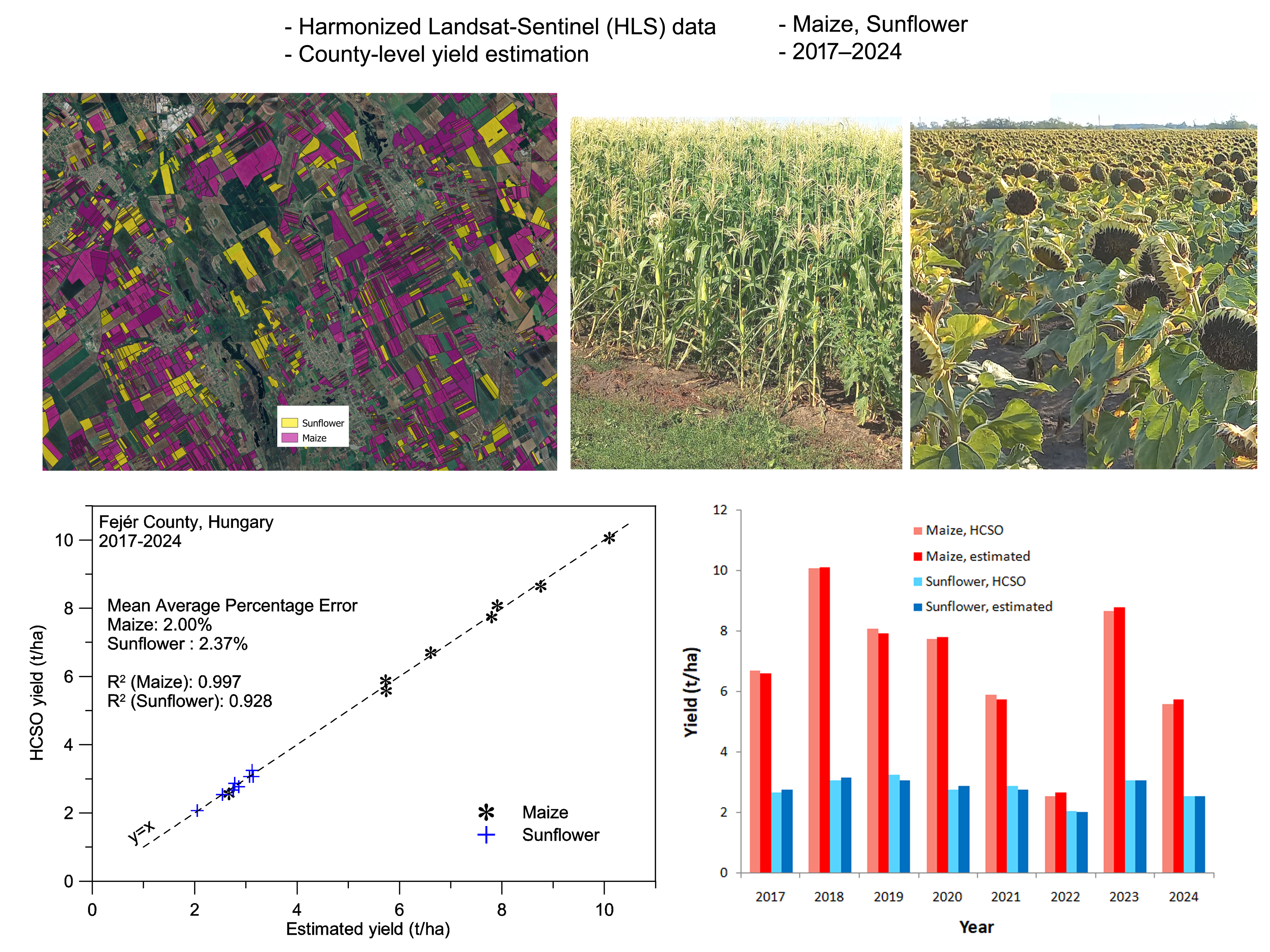
The study area was Fejér County (corresponding to the NUTS (Nomenclature of Territorial Units for Statistics)-3 level), one of the 19 counties of Hungary (Figure 1), located in Central Europe. The county is situated in central Hungary and has a continental climate characterized by relatively warm summers and moderately cold winters. During the study period 2017–2024, the mean annual temperature was 12.3 °C, while the mean summer temperature exceeded 16 °C. The average annual precipitation ranged between 500 and 600 mm [41]. Fejér County covers 4373 km², of which approximately 3000 km² is agricultural land.
In the present study, the two spring-sown row crops with the largest sown areas—maize and sunflower—were investigated. In the 2017–2024 period, the average sown area of maize was 749 km² and that of sunflower was 385 km². The yield data used to validate the yield estimation method (Figure 2) were obtained from the official reports of the HCSO (Hungarian Central Statistical Office) [42].
2.2. Land Cover and Crop Information
The crop yield estimation analysis was performed for agricultural pixels identified using species and habitat type information from the Ecosystem Map of Hungary developed within the NÖSZTÉP (Nemzeti Ökoszisztéma Szolgáltatás-Térképezés és Értékelés) project [43,44]. This map (hereafter referred to as the NÖSZTÉP dataset) distinguishes 56 ecosystem categories (Level 3) at a spatial resolution of 20 m and covers the entire territory of Hungary. The dataset was resampled to the grid of the remote sensing data by summing up the individual shares, resulting in fractional cover values (in percent) for each ecosystem category in every pixel.
To refine our study area and make our method crop-specific, we incorporated crop maps from 2017 to 2024. These maps were provided by the Lechner Knowledge Center [45], and were produced using machine learning methods applied to Sentinel-2 and Sentinel-1 time series with a resolution of 20 meters. They provide detailed information about crop types. Based on these maps, we identified and selected only maize and sunflower pixels for the study. These crops had a precision of around 95% during the study period [46]. Despite using different methods, the areas of the main crops showed good agreement with the values reported by the HCSO [47] (Figure 3). To minimize error, we applied a 20-meter negative buffer to exclude border pixels that could affect our analysis with undesirable edge effects. Then, we resampled the maps for the HLS grid (30 m) and used only those with at least 90% coverage.
2.3. Processing of the HLS Dataset / Calculating County Mean NDVI from HLS Data
The Harmonized Landsat-Sentinel (HLS v2.0) dataset [48,49] was used to calculate NDVI at 30 m spatial resolution for the period 2017–2024. This dataset combines measurements from the OLI on Landsat-8 and Landsat-9 and the MSI on Sentinel-2A and 2B, providing Nadir BRDF (bidirectional reflectance distribution function)-Adjusted Reflectance (NBAR) data at 30 m resolution. Both HLSL30 (Landsat-based) and HLSS30 (Sentinel-based) datasets were downloaded from NASA EarthData Search for the tiles T33TYN and T33TYM in UTM (Universal Transverse Mercator) zone 33, resulting in a total of 2980 granules for the eight years [50].
Pixels were classified as agricultural when the share of agricultural area exceeded 90%. From these data, daily mean NDVI values for Fejér County were calculated separately for Landsat (HLSL30) and Sentinel (HLSS30) datasets, using only the best-quality observations (pixels with low or moderate aerosol content). The calculations were performed for all NÖSZTÉP-based agricultural pixels and, separately, for maize and sunflower fields according to the crop-type information available on the same grid.
2.4. Crop Yield Estimation
In this study, two yield estimation models were developed for Fejér County, covering eight years (2017–2024), based on HLS satellite data. In both cases, the calculations were derived from daily NDVI values averaged over a given area. The two models differ in that, in one case, the data originated from the entire agricultural area of the county, whereas in the other case, a crop-specific mask was applied. The advantage of the first method is that it does not require detailed information on the sown area of each crop, which may vary from year to year. In this approach, it is assumed that the general conditions of vegetation-covered surfaces also represent the conditions of individual crops with similar vegetation cycles [40,51]. The second model, by contrast, requires detailed classification each year to determine the exact sown area of each crop. The first model was previously referred to as the robust method [39], and this terminology is retained in the present study. The second model is hereafter referred to as the crop-specific (CS) model. In the robust procedure, the entire agricultural area of the county was considered, while clearly non-agricultural areas (settlements, forests, large water bodies, etc.) were masked out. The robust model thus minimises data requirements, whereas the CS model incorporates more detailed spatial information but requires accurate annual classification. Subsequently, annual NDVI time series were generated for each crop from the averaged daily NDVI data. As an illustration, Figure 4 presents the NDVI time series for 2024.
As the next step, a double-Gaussian curve was fitted to the annual NDVI time series between appropriately selected starting (tb) and ending (te) days, depending on the crop type, to eliminate stochastic noise caused by atmospheric and other effects [30]:
where G(t) is the fitted double-Gaussian
curve, S is the predefined value of the so-called soil line, A1
and A2 are the amplitudes, t1 and t2
are the locations of the maxima of the Gaussian curves, and h1
and h2 are their respective half-widths. The value of te
corresponds to the date of yield estimation.
The values of the resulting double-Gaussian curve were then
integrated between a suitably selected starting (db) and
ending (de) day, thus obtaining an index that can be directly
compared with the yield data published by the HCSO. It is important to note
that these dates (db and de) are distinct
from the curve-fitting parameters (tb and te).
While the latter are defined based on the beginning and end of the vegetation
period of the given crop, the db and de values
were determined to maximize the correlation between the estimated and actual
yield data (provided by the HCSO). The indices obtained using the CS method
were named GYURI (General Yield Reference Index), and those obtained using the
robust procedure were named GYURRI (General Yield Robust Reference Index) [39]. For example, in the case of GYURI, the value
for a given year y is defined as follows:
where G(t) is the double-Gaussian function
fitted to the daily NDVI data measured in year y for the given crop, and
db and de are the starting and ending dates
of integration. Then, a straight line was fitted to the annual GYURIy
(or GYURRIy) – HCSO point pairs, from whose parameters the
yield for the given year can be simply calculated.
2.5. Statistical Analysis, Diagnostic and Predictive Approach
In this study, we distinguished between diagnostic and
predictive applications of the two above-mentioned yield estimation models. The
diagnostic model aims to describe the relationship between vegetation
index–based indicators (e.g., GYURI) and the observed yields in the
eight years within this study as accurately as possible. The predictive model,
in contrast, aims to estimate future yields under operational conditions, where
the model performance is evaluated by cross-validation (leave-one-year-out) [23,35,52]. This distinction separates the
interpretive value of the method (how yield fluctuations relate to vegetation
dynamics) from its forecasting capability (how well future yields can be
predicted). In the following, we refer to the diagnostic method as R-D for
robust model and CS-D for crop-specific model, while the predictive method as
R-P and CS-P.
The efficiency of the models was tested with three
statistical indicators: square of the Pearson linear correlation coefficient (R2),
mean absolute error (MAE), and mean absolute percentage error (MAPE).
Calculating the correlation coefficient is one of the most commonly used
methods in statistical studies [53], MAE is a widely used metric for evaluating models,
similarly to root mean square error (RMSE) [54,55],
while MAPE is a measure of quality for regression models [56]:
where
and n denotes the number of observations, yi is the observed yield, and ŷiis the
estimated yield.
3. Results
3.1. The Model Parameters for Maize
One of the most important crops in Hungary, and thus in
Fejér county, is maize, whose sown area accounts for approximately 15–20
percent of the total area of the county (Figure 2). The main growing stages for maize in Hungary are the seeding stage
(mid-April to early May), the jointing stage (from mid-May to early June), the
heading stage (from late June to late July), the milking stage (from late July
to mid-August), and the mature stage (from mid-September to early October) [57]. The harvest usually ends around late
September–mid-October. The daily NDVI values of the maize fields determined
based on classification start to increase around DOY (Day Of Year) 120 (end of
April), and then, after reaching maximum values, begin to decrease around DOY
210–220. An exception occurred in 2022, when the extreme late-summer drought
caused an abrupt decline. (Figure 5). By
the end of the harvest (around DOY 260–280), the NDVI values decline to around
0.3. Based on these patterns, the value of soil-line (S) was set to 0.3,
and tb = 125 and te = 260 were chosen as
the starting and final days of curve fitting. This also means that the yield
estimate was made on DOY 260, which typically precedes the end of the harvest
period.
As mentioned in the previous chapter, in this study, four
yield forecasting methods were tested: the R-D, CS-D, R-P, and CS-P models. The
R and CS methods are completely similar; they only differ in the areas from
which the NDVI data originate. Using the robust (R) procedure, these data are
averages for the entire agricultural area, while in the CS method, they are
averages only for areas classified as maize. Consequently, in the R method, the
influence of autumn cereals is obvious in the spring–early summer data (Figure 6), so we examined how the accuracy of
the estimate changes if the starting day of curve fitting (tb)
increases. Experience has shown that it gives better results if the value of tb
is chosen as 140, so this value was used in the case of the R method. The
starting and ending days of the integration (db and de)
used in the calculation of GYURRI in the R-D procedure were 135 and 250,
respectively, while in the CS-D model, the best result was obtained by using db
= 160 and de = 235.
3.2. Results for Maize in the Diagnostic Model
In the eight years studied, maize yields ranged widely,
with the lowest yield in 2022 (2.56 t/ha), which was hit by a late summer
drought, and the highest in 2018 (10.06 t/ha). This wide yield range improved
the robustness of the model calibration, resulting in very high correlation
values, R2 = 0.986 for the R-D method, and R2 = 0.998 for
the CS-D method (Figure 7).
The differences between the estimated and actual HCSO yield
data (Table 1) show that in the case of
the R-D method, the difference exceeded 5% in three of the eight years
examined, the maximum error (6.25%) occurring in the drought year of 2022.
Applying the CS-D model, the differences remained well below 5% in each year,
with the maximum difference being 2.33% in 2024. The CS-D model also performed
reliably under extreme weather conditions: in 2022 the error of the estimation
was only 1.56%. The MAE, that is the average absolute yield difference for the
eight years, is 0.23 t/ha for the R-D model and 0.09 t/ha for the CS-D model,
and the MAPE is 3.78% and 1.37%, respectively.
3.3. Results for Maize in the Predictive Model
The results of the diagnostic model are promising, but it
should not be overlooked that the estimates were calculated based on only eight
data points. Therefore, it is necessary to examine how the results change if
one year is always omitted from the determination of the model parameters, and
the yield of this omitted year is estimated using parameters calculated based
on the remaining seven years. It would be possible to vary the values of db
and de in each case to achieve the best correlation values,
but such adjustments would compromise model stability. Therefore, the same
fixed values of db and de were used for
each year as in the diagnostic model, and only the parameters of the fitted
lines changed from year to year.
The results show (Table 2)
that for the R-P model, the MAE was 0.3 t/ha, while the MAPE value increased to
over 5%. The drought year of 2022 contributed greatly to this, when the
percentage error of the estimate exceeded 16%. In contrast, the CS-P model
yielded substantially better performance. Here, the largest difference between
the estimated and actual yield was 0.17 t/ha in 2019, and even in the drought
year of 2020, the percentage difference did not exceed 5% (4.42%). For the CS-P
model, the MAE was 0.11 t/ha, while the MAPE value was 2%. The correlation
value (R2) of the R-P and CS-P model was 0.976 and 0.997,
respectively (Figure 8). The estimation
results for each year, using the four models, are summarized in Figure 9.
As mentioned above, in predictive models, one year was
always omitted when determining the model parameters. In the case of the CS-P
model, a simulation of an operational yield estimation situation was performed.
In this procedure, the 2020 crop yield was first estimated from the GYURI data
using parameters determined only based on the first three years (2017–2019).
Then, the parameters were determined based on four years (2017–2020), which
would be used to estimate the yield for 2021, and so on. Obviously, the
estimate for 2024 was the same as the result obtained for the CS-P model.
The results (Table 3)
are encouraging; only the year 2022, which had an extremely low yield due to
drought, had a significant error exceeding 10%. It can also be seen that after
including this year, the parameters of the fitted line (a and b)
changed significantly. This also supports the experience that for building a
sufficiently accurate model, it is fortunate that the difference between the
minimum and maximum yield is large enough. While the difference between the
highest and lowest yield in 2017–2021 was 4.18 t/ha, this increased to 7.5 t/ha
after including the year 2022. Interestingly, in the CS-P procedure, when the
2023–2024 data were included in addition to the 2017–2021 data for the 2022
estimate, the error, as mentioned above, turned out to be significantly
smaller. One reason for this is that although the lines fitted to five or seven
years with higher yields differ only slightly, in the low-yield year of 2022,
even this small difference causes a significant percentage difference (Figure 10). This also indicates that model
stability is expected to increase as longer time series become available.
The above results were obtained with an estimate made on
DOY 260. However, examining the evolution of the correlation coefficient (R2)
obtained by changing the te values in the case of the CS-D
model (Figure 11), it appears that it is
possible to provide a sufficiently accurate forecast even at an earlier date.
The calculations were performed for the R-P and CS-P model by simply bringing
the last day of curve fitting (te) forward.
The results showed that the CS-P model obtained significantly
better results than the R-P model (Figure 12).
Using the CS-P model, the MAPE remained below 4% (3.86% to be exact) until DOY
230, about 30–50 days before the end of harvest. Interestingly, in the case of
the CS-P model, the predicted results on DOY 250 were even slightly more
accurate than the estimates obtained on DOY 260. Table 4c shows the numerical results of the
forecast.
3.4. The Model Parameters for Sunflower
Sunflower is the second most important spring crop in
Hungary and Fejér county, with a sowing area of about half that of maize (Figure 3). Annual sunflower and maize yields
showed a moderate positive correlation (Figure 2),
but in the case of sunflower, the fluctuations in yields were much smaller
during the period under study. While the largest positive and negative
deviations from the eight-year average yield for maize were +46% (2018) and
-63% (2022), for sunflower, they were only +17% (2019) and –26% (2022). This
indicates that the severe drought in 2022 affected sunflower yields to a lesser
extent. The growing season of sunflower is roughly the same as that of maize;
the NDVI time series from classified sunflower fields are similar to those
observed for maize, although the autumn decreasing phase of the values begins earlier
(Figure 13). Sunflower harvest generally
begins in late August and lasts until mid-September in Hungary. The timing
depends largely on the weather of the given year; in drier and warmer years,
the harvest season may be shorter, while in cooler, wetter years, it may be
slightly longer depending on the time of sowing and the course of ripening.
Based on these characteristics, the expectation was that the yield estimation
date could be advanced compared to maize.
3.5. Results for Sunflower in the Diagnostic Model
The starting day for fitting the double-Gaussian curve was
chosen as tb = 125, similar to maize. The final date of the
curve-fitting was determined based on the correlation values obtained in the
CS-D model. The highest correlation (R2 = 0.903) was obtained at te
= 230 (Figure 14), which also means that
the yield estimate can be made with sufficient accuracy already in mid-August
(around 18 August).
Given the smaller sown area and lower interannual
variability, a slightly weaker correlation was expected than in the case of
maize. The results confirmed this expectation, although the correlation was
above 0.9 in both the R-D and CS-D cases. Unexpectedly, the R-D model
outperformed the CS-D model. The correlation between the estimated and actual
yields for the R-D method was R2 = 0.954, while for the CS-D model
it was R2 = 0.903 (Figure 15).
The MAE for the R-D method was 0.06 t/ha (MAPE = 2.08%), and for the CS-D
method, it was 0.08 t/ha (MAPE = 2.90%) (Table 5).
In the case of the R-D method, the estimation error remained below 4% in all
years, while in the case of the CS-D model, it was greater than 6% on two
occasions.
3.6. Results for Sunflower in the Predictive Model
The predictive model was applied similarly to the one used
for maize. As with the diagnostic model, the surprising result was that the R-P
model obtained a more accurate estimate than the CS-P model based on purely
sunflower pixels (Table 6).
The predictive performance
exceeded expectations, as the R-P model had only one error of more than 5%
(5.23% in 2019), while the remaining years were below 4%. Moreover, the
estimates for 2023 and 2024 proved to be extremely accurate. Using the CS-P
model, the estimation error exceeded 5% in only two cases. The MAPE value
remained below 4% in both cases, being 2.73% for the R-P model and 3.58% for
the CS-P model. The correlation value for the R-P model was R2 =
0.928, while for the CS-P model it was R2 = 0.864 (Figure 15). The results obtained by the four
models are shown in Figure 16.
Similar to maize, the yield estimate simulating the
operational situation was carried out, but here the R-P method was used. The
results showed that the drought year of 2022 with a very low yield
significantly modified the parameters of estimation, although the estimation of
the yield of this year was just over 5% (Table 7).
Figure 13 indicates that the forecast horizon could not be extended
substantially. In the case of the R-P model, at te = 220, the
percentage difference between the predicted and actual returns was large in two
years (15.3% in 2019 and 9.2% in 2021). However, in the other years, the error
remained below 3.5%, resulting in the MAPE value of 4.08%. A similar result was
obtained in the case of the CS-P model, in which the yield for the year 2019
was also underestimated by 10.3%, and the MAPE value was 4.4%. Forecast
accuracy deteriorated markedly before DOY 220, with the MAPE value at DOY 210
being 9.9% and 7.2% for the R-P and CS-P models, respectively, and at DOY 200
this value increased to over 10% in both cases.
4. Discussion
This study demonstrated the successful application and
refinement of two remote-sensing based yield estimation models for maize and
sunflower using HLS NDVI time series in Fejér County, Hungary. The analysis
covered eight consecutive years (2017–2024), allowing for the evaluation of the
models under diverse weather conditions, including the extreme drought of 2022.
Four modelling configurations were examined: the robust diagnostic (R-D),
crop-specific diagnostic (CS-D), robust predictive (R-P) and crop-specific
predictive (CS-P) models. The input data for the robust methods were the daily
county-level means of NDVI, calculated over all agricultural pixels, whereas
the crop-specific models used NDVI values extracted only from pure maize and
sunflower fields. In the latter case, the classification had to be done
accurately every year. While the diagnostic models relied on all eight years to
establish the NDVI–yield relationships, the predictive models employed
leave-one-year-out cross-validation to emulate operational forecasting
conditions. This distinction made it possible to assess both the interpretive
value and the practical forecasting skill of the modelling framework. From a
practical point of view, the predictive model is more important, as this procedure
is closer to the real, operational situation, where model parameters calculated
based on previous years must be used to estimate the yield of the current year.
For maize, all models
achieved very high accuracy, the correlation coefficient (R²) was 0.976 for the
R-P model and 0.997 for the CS-P model, indicating excellent agreement in both
cases but with a measurable advantage for the crop-specific approach. Using the
CS-P model, the MAE value was 0.11 t/ha (RMSE = 0.12 t/ha) and the MAPE was
2.0%.
For the above results, yield estimation was performed
approximately at the beginning of the crop harvest, in late September, on DOY
260. Importantly, forecast accuracy remained high even when predictions were
made on DOY 230, mid-August, 30–50 days before the end of harvest, when using
the CS-P model, the MAPE was 3.86%.
For sunflower, the modelling outcomes showed an unexpected
pattern: the robust models outperformed the crop-specific ones. The R-P model
reached an R² = 0.928, the MAE was 0.08 t/ha (RMSE = 0.09 t/ha), and the MAPE
was 2.73%, while the CS-P model produced somewhat weaker results with R² = 0.866,
MAE = 0.10 t/ha (RMSE = 0.13 t/ha), and MAPE = 3.58%. Notably, both models
accurately captured the low yields of 2022, with the difference between the
estimated and actual yield being 2.5% for the R-P model and only 0.5% for the
CS-P model. Simulating a quasi-operational situation using the robust
procedure, the results remained consistently reliable. The difference between
the estimated and actual yield is 0.03% in 2023 and 0.16% in 2024. However, the
robust models performed more consistently for sunflower, despite the
crop-specific models using only sunflower pixels, and this difference warrants
additional analysis. The statistical results of the four models are summarized
in Table 8.
For comparison, Skakun et al. [58]
estimated maize yields at sub-field scales within study sites in the US state
of Iowa, and observed mixed performance of satellite-derived models with the R²
varying from 0.21 to 0.88 (averaging 0.56) for the HLS. Khaki et al. [59] used data from 1132 counties for maize across
the United States, and predicted the yield one to four months before the
harvest, with the MAPE being 8.74%. In the work of Kumar et al. [60], regression analysis was developed between
observed yield from crop cut experimental plots and seasonal maximum NDVI of
maize area using Sentinel-2 data in India, and a significant relation (R² = 0.87)
was obtained between NDVI and observed yield at respective field plots. Wang et
al. [61] used Sentinel-2A and MODIS data to
construct a yield forecasting model for summer maize in China, with the MAPE
being 5.47%–13.74%. The experiment of Gavilán et al. [62]
based on Sentinel-2 data was carried out in maize fields located in the
Argentine Pampas Region in summer (from January to March) of 2020, obtaining a
high (R² = 0.91) correlation value. Birinyi et al. [63]
used a six-category crop condition mapping method based on Sentinel-2 data,
which explained 77% of county-level yield variability for maize in July. Adriko
et al. [64] compared results based on MODIS
and Sentinel-2 data in the Midwestern corn belt in the United States; the
correlation value was R² = 0.79 for Sentinel-2 and R² = 0.87 for MODIS. Radocaj
et al. [65] analyzed Sentinel-2 vegetation
index time-series and phenology metrics for Iowa and Illinois, and reported
that the combination of wide dynamic range vegetation index and the
maximum-value metric achieved the strongest relationship with maize yield, with
a mean correlation of about 0.51. In the case of sunflower, Narin et al. [66] obtained R² = 0.74 approximately three months
before the harvest in Turkey using Sentinel-2 data. Amankukova et al. [67] applied multiple linear regression and two
different machine learning approaches to predicting the crop yield using
Sentinel-2 data. They found that the most suitable time for predicting the crop
yield was 86–116 days after sowing, the best machine learning approach for
predicting field-scale variability of the crop yield was about R² = 0.6 and
RMSE = 0.284–0.473 t/ha.
Despite methodological differences, the county-level
performance of our models achieved similar or better explanatory power through
a simpler, continuous NDVI-based regression model, thereby reducing model
complexity and computational cost.
5. Conclusions
In our current research, we had four main objectives: (i)
to improve the previously developed robust method based on 30-m data, (ii) to
test the model on input data from areas with different vegetation cover, (iii)
to estimate the predictive power of the model, and (iv) to test the accuracy of
the model for forecasts at different dates. Our results demonstrate that these
objectives were successfully achieved through the combined use of HLS data, and
regression-based yield models. Both the robust and the crop-specific approaches
provided stable and reliable performance, although with different advantages.
In the case of maize, the crop-specific model provided a more accurate
estimate; however, due to its simplicity and low data requirements, the robust
model can be more suitable where a detailed annual crop map is limited or unavailable.
Importantly, the models responded well even under extreme growing season
conditions, such as the drought year of 2022, highlighting their resilience to
increasing climate variability.
Testing the predictive model, it was found that maize
yields can be forecast with high accuracy as early as 30–50 days before the end
of harvest, which represents significant value for operational decision-making.
For sunflower, the early-season forecasting proved more limited; nevertheless,
both models maintained reliable accuracy on DOY 230, around the typical
beginning of the harvest. Overall, the presented approach offers a favourable
balance between model simplicity, data requirements and predictive ability,
outperforming or matching the results of more complex methods reported in the
literature while requiring fewer input variables. The results also confirm that
dense NDVI time series derived from HLS data are suitable for operational
regional-scale yield forecasting. Consequently, the methodology can clearly be integrated
into regional or national early warning systems. Future research may extend
this work to additional crop types and incorporate meteorological or soil
moisture information to increase the accuracy and generalizability of the
model. It would also be important to include additional years in the studies so
that longer time series enhance the stability of the model.
Funding
The research has been supported by the Hungarian National Scientific Research Fund (NKFIH FK-146600) and the TKP2021-NVA-29 project of the Hungarian National Research, Development and Innovation Fund, with the support provided by the Ministry of Culture and Innovation of Hungary. This work was implemented by the National Multidisciplinary Laboratory for Climate Change (RRF-2.3.1-21-2022-00014) project within the framework of Hungary's National Recovery and Resilience Plan, supported by the Recovery and Resilience Facility of the European Union.
Data availability Statement
The data presented in this study are available from the corresponding author, upon
reasonable request.
Conflicts of Interest
The authors declare no conflicts of interest.
Abbreviations
The following abbreviations are used in this
manuscript:
| NDVI | Normalized difference vegetation index |
| HLS | Harmonized Landsat-Sentinel |
| NOAA | National Oceanic and Atmospheric Administration |
| AVHRR | Advanced Very High Resolution Radiometer |
| NASA | National Aeronautics and Space Administration |
| MODIS | Moderate Resolution Imaging Spectroradiometer |
| OLI | Operational Land Imager |
| MSI | MultiSpectral Instrument |
| HCSO | Hungarian Central Statistical Office |
| NUTS | Nomenclature of Territorial Units for Statistics |
| UTM | Universal Transverse Mercator |
| BRDF | Bidirectional reflectance distribution function |
| NÖSZTÉP | Nemzeti ökoszisztéma szolgáltatás-térképezés és értékelés |
| RMSE | Root mean square error |
| MAE | Mean absolute error |
| MAPE | Mean absolute percentage error |
| GYURI | General Yield Reference Index |
| GYURRI | General Yield Robust Reference Index |
| DOY | Day of year |
| CS-D | Crop-specific diagnostic |
| CS-P | Crop-specific predictive |
| R-D | Robust/diagnostic |
| R-P | Robust/predictive |
References
- Wahla, S.S.; Kazmi, J.H.; Sharifi, A.; Shirazi, S.A.; Tariq, A.; Smith, H.J. Assessing spatio-temporal mapping and monitoring of climatic variability using SPEI and RF machine learning models. Geocarto Int. 2022, 37(27), 14963–14982. [Google Scholar] [CrossRef]
- Sharifi, A.; Mahdipour, H.; Moradi, E.; Tariq, A. Agricultural field extraction with deep learning algorithm and satellite imagery. J. Indian Society and Remote Sens. 2022, 50, 417–423. [Google Scholar] [CrossRef]
- Becker-Reshef, I.; Barker, B.; Humber, M.; Puricelli, E.; Sanchez, A.; Sahajpal, R.; Mcgaughey, K.; Justice, C.; Baruth, B.; Wu, B.; et al. The GEOGLAM crop monitor for AMIS: Assessing crop conditions in the context of global markets. Global Food Secur. 2019, 23, 173–181. [Google Scholar] [CrossRef]
- Skakun, S.; Kalecinski, N.I.; Brown, M.G.L.; Johnson, D.M.; Vermote, E.F.; Roger, J.-C.; Franch, B. Assessing within-field corn and soybean yield variability from WorldView-3, Planet, Sentinel-2, and Landsat 8 satellite imagery. Remote Sens. 2021, 13, 872 . [Google Scholar] [CrossRef]
- Xiao, G.; Huang, J.; Zhuo, W.; Huang, H.; Song, J.; Du, K. Progress and perspectives of crop yield forecasting with remote sensing: A review. IEEE Geosci. and Remote Sens. Mag. 2025, 13(3), 338–368. [Google Scholar] [CrossRef]
- Khanal, S.; Kushal, K.C.; Fulton, J P. ; Shearer, S.; Ozkan, E. Remote sensing in agriculture—Accomplishments, limitations, and opportunities. Remote Sens. 2020, 12, 3783. [Google Scholar] [CrossRef]
- Atzberger, C. Advances in remote sensing of agriculture: Context description, existing operational monitoring systems and major information needs. Remote Sens. 2013, 5, 949–981. [Google Scholar] [CrossRef]
- Kalecinski, N I. ; Skakun, S.; Torbick, N.; Huang, X.; Franch, B.; Roger, J.-C.; Vermote, E. Crop yield estimation at different growing stages using a synergy of SAR and optical remote sensing data. Science of Remote Sens. 2024, 10, 100153. [Google Scholar] [CrossRef]
- Gomez, D.; Salvador, P.; Sanz, J.; Casanova, J.L. Modelling wheat yield with antecedent information, satellite and climate data using machine learning methods in Mexico. Agric. For. Meteorol. 2021, 300, 108317. [Google Scholar] [CrossRef]
- Zhang, H.; Zhang, Y.; Liu, K.; Lan, S.; Gao, T.; Li, M. Winter wheat yield prediction using integrated Landsat 8 and Sentinel-2 vegetation index time-series data and machine learning algorithms. Comput. Electron. Agric. 2023, 213, 108250. [Google Scholar] [CrossRef]
- Kasampalis, D.; Alexandridis, T.; Deva, C.; Challinor, A.; Moshou, D.; Zalidis, G. Contribution of remote sensing on crop models: A review. J. Imaging 2018, 4, 52. [Google Scholar] [CrossRef]
- Rahman, M.M.; Robson, A. Integrating Landsat-8 and Sentinel-2 time series data for yield prediction of sugarcane crops at the block level. Remote Sens. 2020, 12, 1313. [Google Scholar] [CrossRef]
- Drusch, M.; Del Bello, U.; Carlier, S.; Colin, O.; Fernandez, V.; Gascon, F.; Hoersch, B.; Isola, C.; Laberinti, P.; Martimort, P.; et al. Sentinel-2: ESA’s optical high-resolution mission for GMES operational services. Remote Sens. Environ. 2012, 120, 25–36. [Google Scholar] [CrossRef]
- Irons, J.R.; Dwyer, J.L.; Barsi, J.A. The next Landsat satellite: The Landsat data continuity mission. Remote Sens. Environ. 2012, 122, 11–21. [Google Scholar] [CrossRef]
- Choate, M.J.; Rengarajan, R.; Hasan, N.; Denevan, A.; Ruslander, K. Operational aspects of Landsat 8 and 9 geometry. Remote Sens. 2023, 16, 133. [Google Scholar] [CrossRef]
- Knight, E.J.; Kvaran, G. Landsat-8 Operational Land Imager design, characterization and performance. Remote Sens. 2014, 6(11), 10286–10305. [Google Scholar] [CrossRef]
- Xu, H.; Ren, M.; Lin, M. Cross-comparison of Landsat-8 and Landsat-9 data: A three-level approach based on underfly images. GISci. Remote Sens. 2024, 61. [Google Scholar] [CrossRef]
- Brown, M.E. ; Pinzón, J E.; Didan, K.; Morisette, J.T.; Tucker, C.J. Evaluation of the consistency of long-term NDVI time series derived from AVHRR, SPOT-vegetation, SeaWiFS, MODIS, and Landsat ETM+ sensors. IEEE Trans. Geosci. Remote Sens. 2006, 44, 1787–1793. [Google Scholar] [CrossRef]
- Fensholt, R.; Rasmussen, K.; Nielsen, T.T.; Mbow, C. Evaluation of earth observation based long term vegetation trends—Intercomparing NDVI time series trend analysis consistency of Sahel from AVHRR GIMMS, Terra MODIS and SPOT VGT data. Remote Sens. Environ. 2009, 113, 1886–1898. [Google Scholar] [CrossRef]
- Kovalsky, V.; Roy, D P. The global availability of Landsat 5 TM and Landsat 7 ETM+ land surface observations and implications for global 30 m Landsat data product generation. Remote Sens. Environ. 2013, 130, 280–293. [Google Scholar] [CrossRef]
- Claverie, M.; Ju, J.; Masek, J.G. ; Dungan, J L.; Vermote, E.F.; Roger, J.-C.; Skakun, S.V.; Justice, C. The harmonized Landsat and Sentinel-2 surface reflectance data set. Remote Sens. Environ. 2018, 219, 145–161. [Google Scholar] [CrossRef]
- Jia, K.; Hasan, U.; Jiang, H.; Qin, B.; Chen, S.; Li, D.; Wang, C.; Deng, Y.; Shen, J. How frequent the Landsat 8/9-Sentinel 2A/B virtual constellation observed the Earth for continuous time series monitoring. Int. J. Appl. Earth Obs. Geoinf. 2024, 130, 103899. [Google Scholar] [CrossRef]
- Skakun, S.; Vermote, E.; Franch, B.; Roger, J.-C.; Kussul, N.; Ju, J.; Masek, J. Winter wheat yield assessment from Landsat 8 and Sentinel-2 data: incorporating surface reflectance, through phenological fitting, into regression yield models. Remote Sens. 2019, 11(15), 1768. [Google Scholar] [CrossRef]
- Zhang, H.; Zhang, Y.; Liu, K.; Lan, S.; Gao, T.; Li, M. Winter wheat yield prediction using integrated Landsat 8 and Sentinel-2 vegetation index time-series data and machine learning algorithms. Comput. Electron. Agric. 2023, 213, 108250. [Google Scholar] [CrossRef]
- Li, M.; Wang, P.; Tansey, K.; Zhang, Y.; Guo, F.; Liu, J.; Li, H. An interpretable wheat yield estimation model using an attention mechanism-based deep learning framework with multiple remotely sensed variables. Int. J. Appl. Earth Obs. Geoinf. 2025, 140, 104579. [Google Scholar] [CrossRef]
- Ren, S.; Guo, B.; Wu, X.; Zhang, L.; Ji, M.; Wang, J. Winter wheat planted area monitoring and yield modeling using MODIS data in the Huang-Huai-Hai Plain, China. Comput. Electron. Agric. 2021, 182, 106049. [Google Scholar] [CrossRef]
- Feng, D.; Yang, H.; Gao, K.; Jin, X.; Li, Z.; Nie, C.; Zhang, G.; Fang, L.; Zhou, L.; Guo, H.; et al. Time-series NDVI and greenness spectral indices in mid-to-late growth stages enhance maize yield estimation. Field Crops Res. 2025, 333, 110069. [Google Scholar] [CrossRef]
- Peng, B.; Guan, K.; Zhou, W.; Jiang, C.; Frankenberg, C.; Sun, Y.; He, L.; Köhler, P. Assessing the benefit of satellite-based solar-induced chlorophyll fluorescence in crop yield prediction. Int. J. Appl. Earth Obs. Geoinf. 2020, 90, 102126. [Google Scholar] [CrossRef]
- Li, C.; Zhang, L.; Wu, X.; Chai, H.; Xiang, H.; Jiao, Y. Winter wheat yield estimation by fusing CNN–MALSTM deep learning with remote sensing indices. Agriculture 2024, 14(11), 1961. [Google Scholar] [CrossRef]
- Maselli, F.; Conese, C.; Petkov, L.; Gilabert, M.A. Use of NOAA–AVHRR NDVI data for environmental monitoring of crop forecasting in the Sahel: Preliminary results. Int. J. Remote Sens. 1992, 13, 2743–2749. [Google Scholar] [CrossRef]
- Hamar, D.; Ferencz, C.; Lichtenberger, J.; Tarcsai, G.; Ferencz-Árkos, I. Yield estimation for corn and wheat in the Hungarian Great Plain using Landsat MSS data. Int. J. Remote Sens. 1996, 17, 1689–1699. [Google Scholar] [CrossRef]
- Moriondo, M.; Maselli, F.; Bindi, M. A simple model of regional wheat yield based on NDVI data. Eur. J. Agron. 2007, 26(3), 266–274. [Google Scholar] [CrossRef]
- Schut, A.G.T.; Stephens, D.J.; Stovold, R.G.H.; Adams, M.; Craig, R.L. Improved wheat yield and production forecasting with a moisture stress index, AVHRR and MODIS data. Crop Pasture Sci. 2009, 60, 60–70. [Google Scholar] [CrossRef]
- López-Lozano, R.; Duveiller, G.; Seguini, L.; Meroni, M.; García-Condado, S.; Hooker, J.; Leo, O.; Baruth, B. Towards regional grain yield forecasting with 1 km-resolution EO biophysical products: Strengths and limitations at Pan-European level. Agric. For. Meteorol. 2015, 206, 12–32. [Google Scholar] [CrossRef]
- Kern, A.; Barcza, Z.; Marjanovic, H.; Árendás, T.; Fodor, N.; Bónis, P.; Bognár, P.; Lichtenberger, J. Statistical modelling of crop yield in Central Europe using climate data and remote sensing vegetation indices. Agric. For. Meteorol. 2018, 260–261, 300–320. [Google Scholar] [CrossRef]
- Johnson, D.; Rosales, A.; Mueller, R.; Reynolds, C.; Frantz, R.; Anyamba, A.; Pak, E.; Tucker, C. USA crop yield estimation with MODIS NDVI: Are remotely sensed models better than simple trend analyses? Remote Sens. 2021, 13, 4227. [Google Scholar] [CrossRef]
- Basso, B.; Cammarano, D.; Carfagna, E. Review of crop yield forecasting methods and early warning systems. In Proceedings of the First Meeting of the Scientific Advisory Committee of the Global Strategy to Improve Agricultural and Rural Statistics; Rome, Italy; 2013; pp. 15–31. [Google Scholar]
- Zeng, Y.; Hao, D.; Huete, A.; Dechant, B.; Berry, J.; Chen, J.M.; Ryu, Y.; Xiao, J.; Ghassem, R. A.; Chen, M. Optical vegetation indices for monitoring terrestrial ecosystems globally. Nat. Rev. Earth Environ. 2022, 3, 477–493. [Google Scholar] [CrossRef]
- Ferencz, C.; Bognár, P.; Lichtenberger, J.; Hamar, D.; Tarcsai, G.; Timár, G.; Molnár, G.; Pásztor, S.; Székely, B.; Ferencz, O. E.; et al. Crop yield estimation by satellite remote sensing. Int. J. Remote Sens. 2004, 25, 4113–4149. [Google Scholar] [CrossRef]
- Bognár, P.; Kern, A.; Pásztor, S.; Lichtenberger, J.; Koronczay, D.; Ferencz, C. Yield estimation and forecasting for winter wheat in Hungary using time series of MODIS data. Int. J. Remote Sens. 2017, 38, 3394–3414. [Google Scholar] [CrossRef]
- Kern, A.; Dobor, L.; Hollós, R.; Marjanovic, H.; Torma, Cs.Zs.; Kis, A.; Fodor, N.; Barcza, Z. ; Seamlessly combined historical and projected daily meteorological datasets for impact studies in Central Europe: the FORESEE v4.0 and the FORESEE-HUN v1.0. Clim. Serv. 2024, 33, 100443. [Google Scholar] [CrossRef]
- HCSO. Available online: https://www.ksh.hu/stadat_files/mez/en/mez0072.html (accessed on 6 November 2025).
- Tanács, E.; Belényesi, M.; Lehoczki, R.; Pataki, R.; Petrik, O.; Standovár, T.; Pásztor, L.; Laborczi, A.; Szatmári, G.; Molnár, Z.; et al. A national, high-resolution ecosystem basemap: Methodology, validation, and possible uses. Természetvédelmi Közlemények 2019, 25, 34–58. [Google Scholar] [CrossRef]
- NÖSZTÉP Ecosystem Map of Hungary. Available online: https://alapterkep.termeszetem.hu/ (accessed on 14 November 2020).
- Kristóf, D.; Petrik, O.; Pataki, R.; Lehoczki, R.; Belényesi, M.; Friedl, Z.; Nádor, G., Hubik, I.; Rotterné Kulcsár, A.; Birinyi, E.; et al. Combined use of EO imagery and in situ data for country-wide land cover mapping and monitoring for various applications in Hungary: Status and perspectives. In Proceedings of the ESA Living Planet Symposium, Milan, Italy, 13–17 May 2019.
- Pacskó, V.; Belényesi, M.; Barcza, Z. Vetésszerkezeti térképek idősorának kategóriánkénti pontosságvizsgálata. In Az elmélet és gyakorlat találkozása a térinformatikában XIV; Debreceni Egyetemi Kiadó, Hungary, 2023; pp. 191-198. ISBN 978-963-615-084-6. https://giskonferencia.unideb.hu/arch/GIS_Konf_kotet_2023.pdf.
- Pacskó, V.; Belényesi, M.; Barcza, Z. Távérzékelés alapú vetésszerkezeti térképek és KSH földterület adatok összehasonlító elemzésének első eredményei. Presented at the Fény-Tér-Kép, Visegrád, Hungary, 5-6 October 2023. 6 October.
- Masek, J.; Ju, J.; Roger, J.; Skakun, S.; Vermote, E.; Claverie, M.; Dungan, J.; Yin, Z.; Freitag, B.; Justice, C. HLS Sentinel-2 Multi-spectral Instrument Surface Reflectance Daily Global 30 m v2.0. Distributed by NASA EOSDIS Land Processes Distributed Active Archive Center, 2021. [CrossRef]
- Masek, J.; Ju, J.; Roger, J.; Skakun, S.; Vermote, E.; Claverie, M.; Dungan, J.; Yin, Z.; Freitag, B.; Justice, C. ; HLS Operational Land Imager Surface Reflectance and TOA Brightness Daily Global 30m v2.0. Distributed by NASA EOSDIS Land Processes Distributed Active Archive Center, 2021. [CrossRef]
- EarthDataSearch, 2025. Available online: https://search.earthdata.nasa.gov/ (accessed on 4 February 2025).
- Dabrowska-Zielińska, K.; Kogan, F.; Ciolkosz, A.; Gruszczyńska, M.; Kowalik, W. Modelling of crop growth conditions and crop yield in Poland using AVHRR-based indices. Int. J. Remote Sens. 2002, 23, 1109–1123. [Google Scholar] [CrossRef]
- Cawley, G.C.; Talbot, N.L.C. Fast exact leave-one-out cross-validation of sparse least-squares support vector machines. Neural Networks 2004, 17(10), 1467–1475. [Google Scholar] [CrossRef]
- Bewick, V.; Cheek, L.; Ball, J. Statistical review 7: Correlation and regression. Crit. Care 2003, 7(6), 451–459. [Google Scholar] [CrossRef] [PubMed]
- Willmott, C.J.; Matsuura, K. Advantages of the mean absolute error (MAE) over the root mean square error (RMSE) in assessing average model performance. Clim. Res. 2005, 30, 79–82. [Google Scholar] [CrossRef]
- Hodson, T.O. Root-mean-square error (RMSE) or mean absolute error (MAE): When to use them or not. Geosci. Model Dev. 2022, 15, 5481–5487. [Google Scholar] [CrossRef]
- De Myttenaere, A.; Golden, B.; Le Grand, B.; Rossi, F. Mean absolute percentage error for regression models. Neurocomputing 2016, 192, 38–48. [Google Scholar] [CrossRef]
- Nyéky, A.; Daróczy, B.; Neményi, M.; Ambrus, B.; Teschner, G.; Alahmad, T. Predicting maize growth and biomass: Integrating gradient boosted trees with Sentinel images and IoT. Progress Agricult. Sci. 2025. [CrossRef]
- Skakun, S.; Kalecinski, N I. ; Brown, M.G.L.; Johnson, D.M.; Vermote, E F.; Roger, J.-C.; Franch, B. Assessing within-field corn and soybean yield variability from WorldView-3, Planet, Sentinel-2, and Landsat 8 satellite imagery. Remote Sens. 2021, 13, 872. [Google Scholar] [CrossRef]
- Khaki, S.; Pham, H.; Wang, L. Simultaneous corn and soybean yield prediction from remote sensing data using deep transfer learning. Sci. Rep. 2021, 11, 11132. [Google Scholar] [CrossRef] [PubMed]
- Kumar, D A.; Neelima, T L.; Srikanth, P.; Devi, M.U.; Suresh, K.; Murthy, C.S. Maize yield prediction using NDVI derived from Sentinel-2 data in Siddipet district of Telangana state. J. Agrometeorol. 2022, 24, 165–168. [CrossRef]
- Wang, J.; He, P.; Liu, Z.; Jing, Y.; Bi, R. Yield estimation of summer maize based on multi-source remote-sensing data. Agron. J. 2022, 14, 3389–3406. [Google Scholar] [CrossRef]
- Gavilán, S.; Aceñolaza, P.G.; Pastore, J.I. Maize (Zea mays L.) yield estimation using high spatial and temporal resolution Sentinel-2 remote sensing data. Commun. Soil Sci. Plant Anal. 2023, 54, 2045–2058. [Google Scholar] [CrossRef]
- Birinyi, E.; Kristóf, D.; Hollós, R.; Barcza, Z.; Kern, A. Large-scale maize condition mapping to support agricultural risk management. Remote Sens. 2024, 16(24), 4672. [Google Scholar] [CrossRef]
- Adriko, K.; Sedona, R.; Seguini, L.; Riedel, M.; Cavallaro, G.; Paris, C. From MODIS to Sentinel-2: A regional comparative analysis of crop-yield prediction with matched spatiotemporal data. IEEE J. Sel. Top. Appl. Earth Obs. Remote Sens. 2025, 18, 27663–27683. [Google Scholar] [CrossRef]
- Radocaj, D; Jurišić, M. A Phenology-Based Evaluation of the Optimal Proxy for Cropland Suitability Based on Crop Yield Correlations from Sentinel-2 Image Time-Series. Agricult. 2025, 15, 859. [CrossRef]
- Narin, O.G.; Abdikan, S. Monitoring of phenological stage and yield estimation of sunflower plant using Sentinel-2 satellite images. Geocarto Int. 2020, 37(5), 1378–1392. [Google Scholar] [CrossRef]
- Amankulova, K.; Farmonov, N.; Mukhtorov, U.; Mucsi, L. Sunflower crop yield prediction by advanced statistical modeling using satellite-derived vegetation indices and crop phenology. Geocarto Int. 2023, 38(1), 2197509. [Google Scholar] [CrossRef]
Figure 1.
The study area: Fejér County, Hungary.
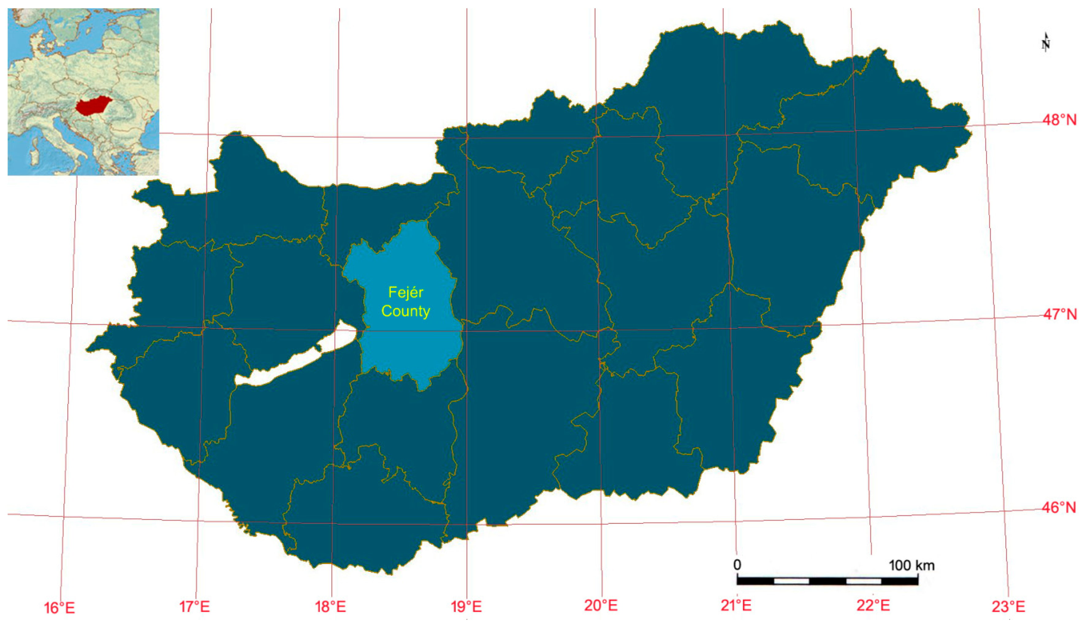
Figure 2.
The Hungarian Central Statistical Office (HCSO) yields of maize and sunflower between 2017–2024.
Figure 2.
The Hungarian Central Statistical Office (HCSO) yields of maize and sunflower between 2017–2024.
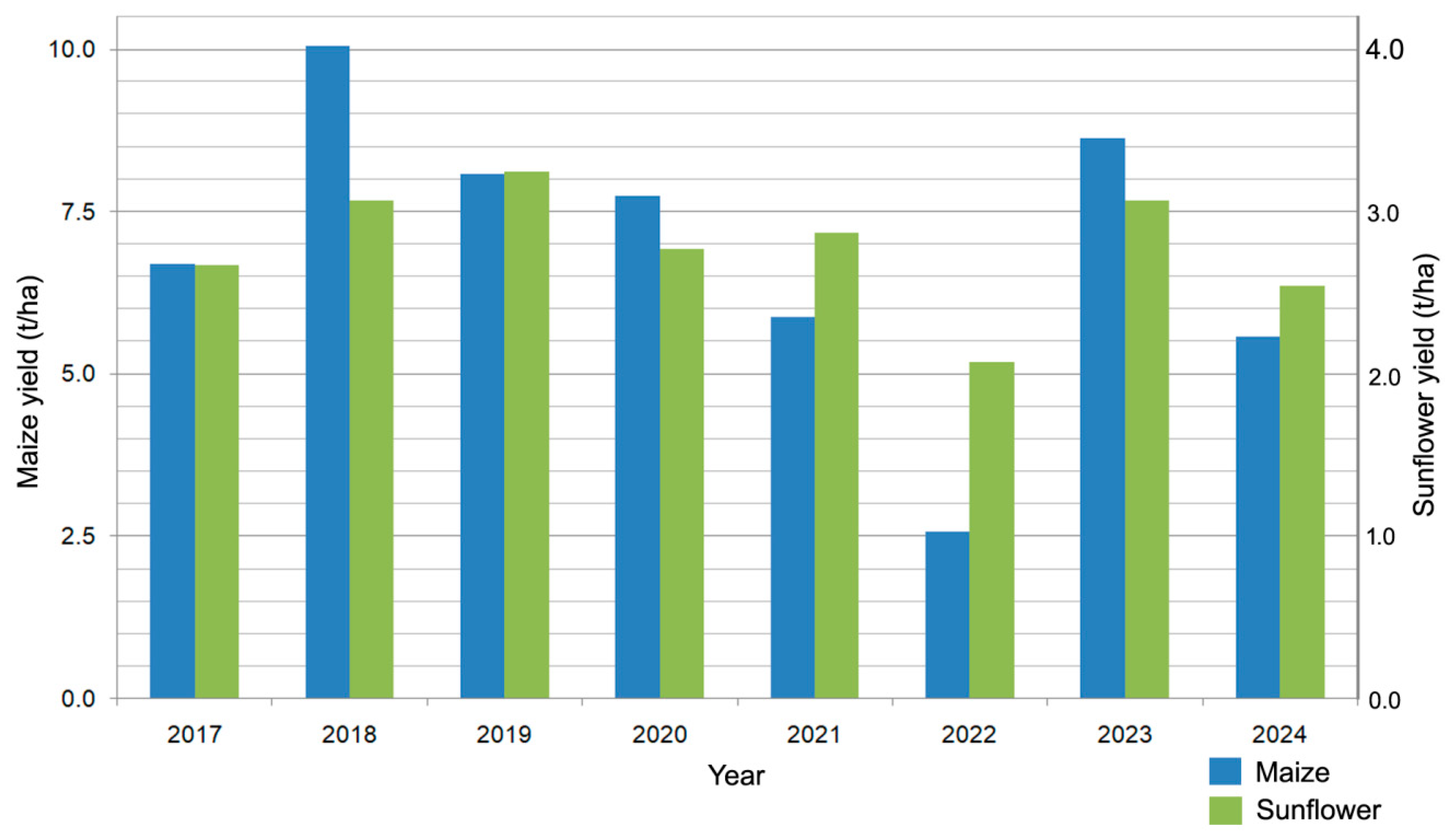
Figure 3.
The proportion of the sowing area of maize and sunflower in Fejér County, based on classification (cl.) results and HCSO data.
Figure 3.
The proportion of the sowing area of maize and sunflower in Fejér County, based on classification (cl.) results and HCSO data.
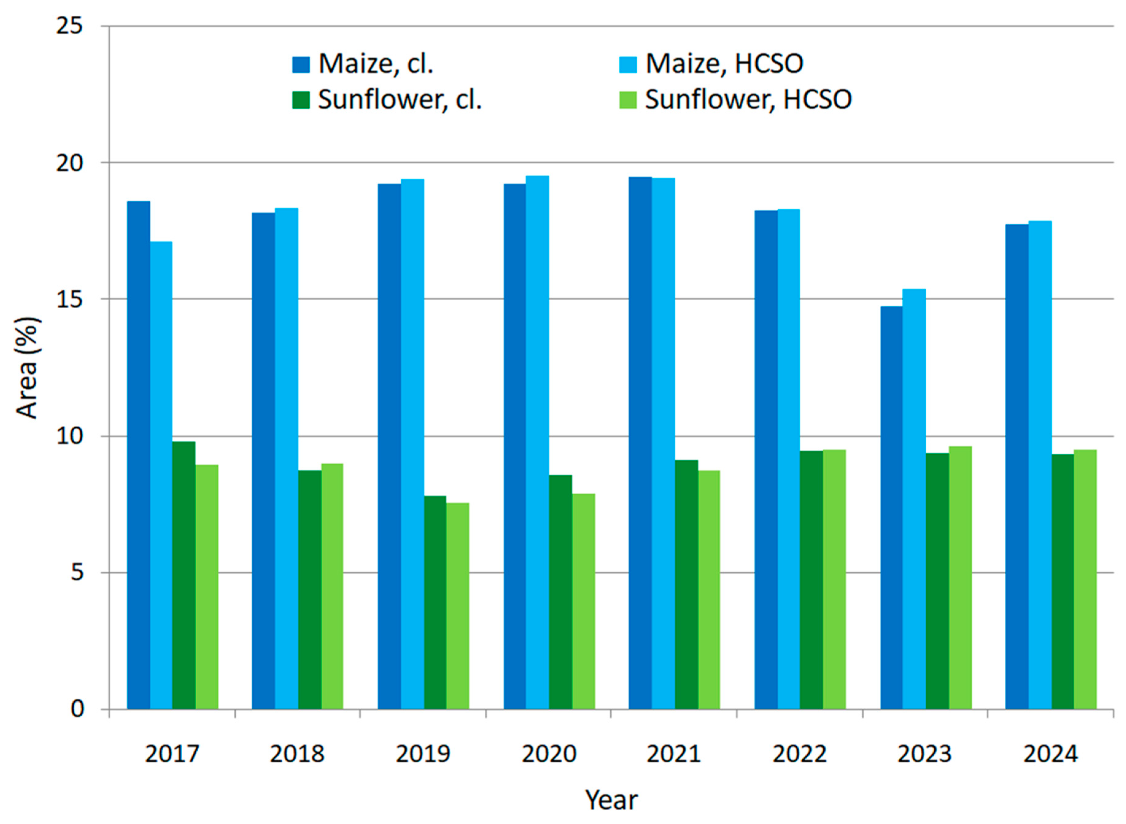
Figure 4.
Example Normalized Difference Vegetation Index (NDVI) time series in 2024.
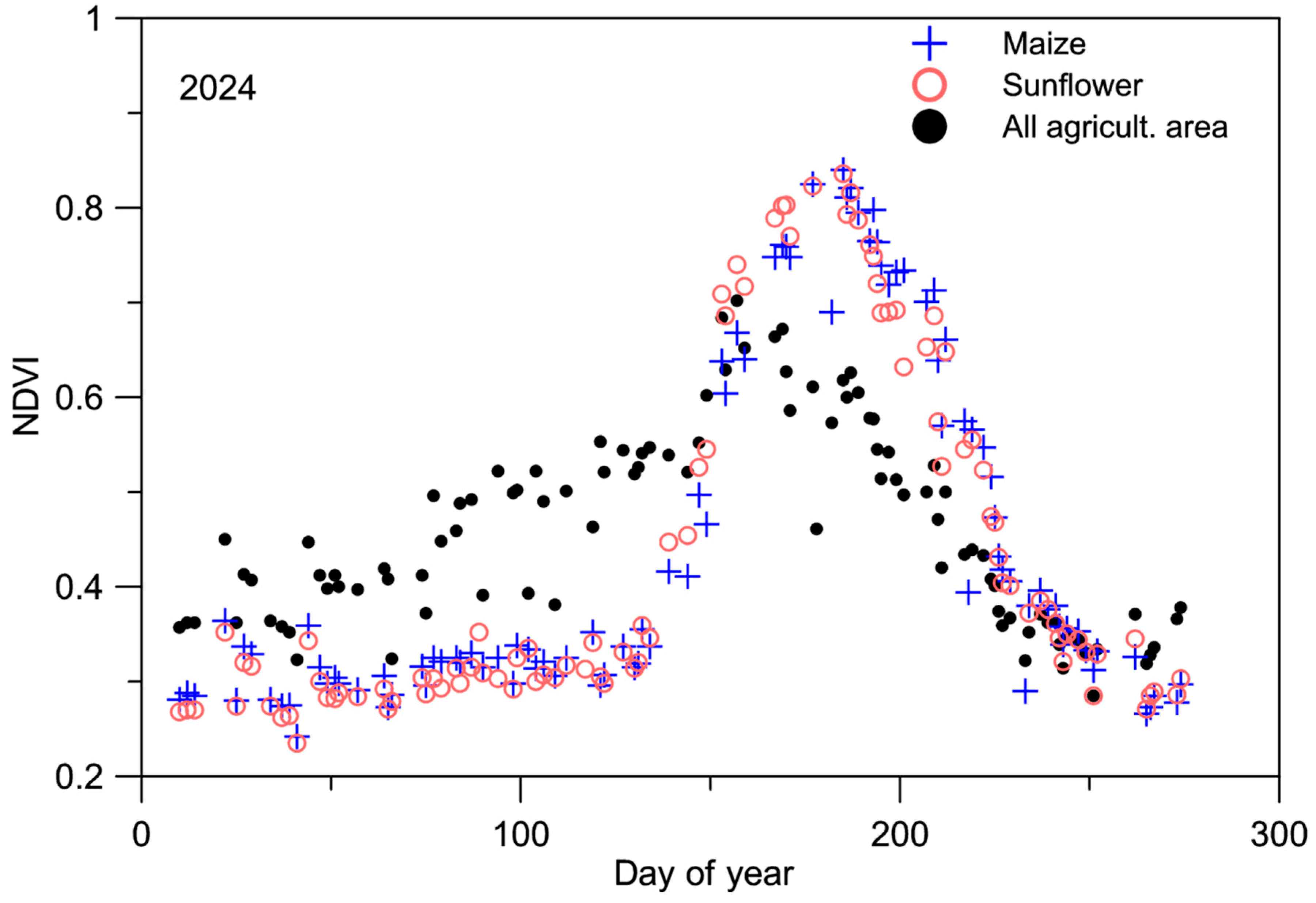
Figure 5.
The daily NDVI values of maize fields in 2017 (normal year) and 2022 (drought year).
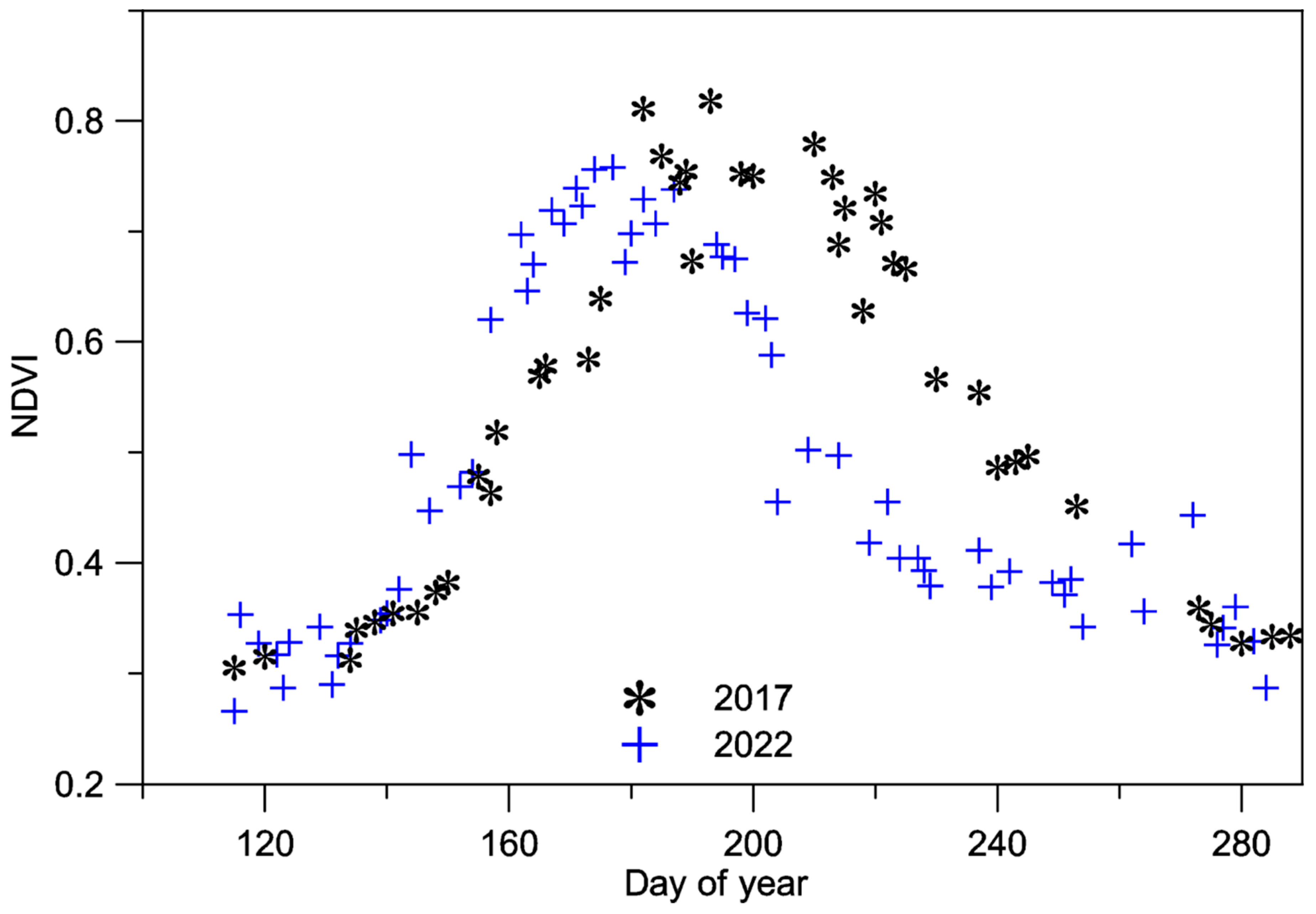
Figure 6.
The average NDVI data of maize fields and the whole agricultural area with the fitted double-Gaussian curves in 2021. The fainter points were not taken into account in the curve fitting.
Figure 6.
The average NDVI data of maize fields and the whole agricultural area with the fitted double-Gaussian curves in 2021. The fainter points were not taken into account in the curve fitting.
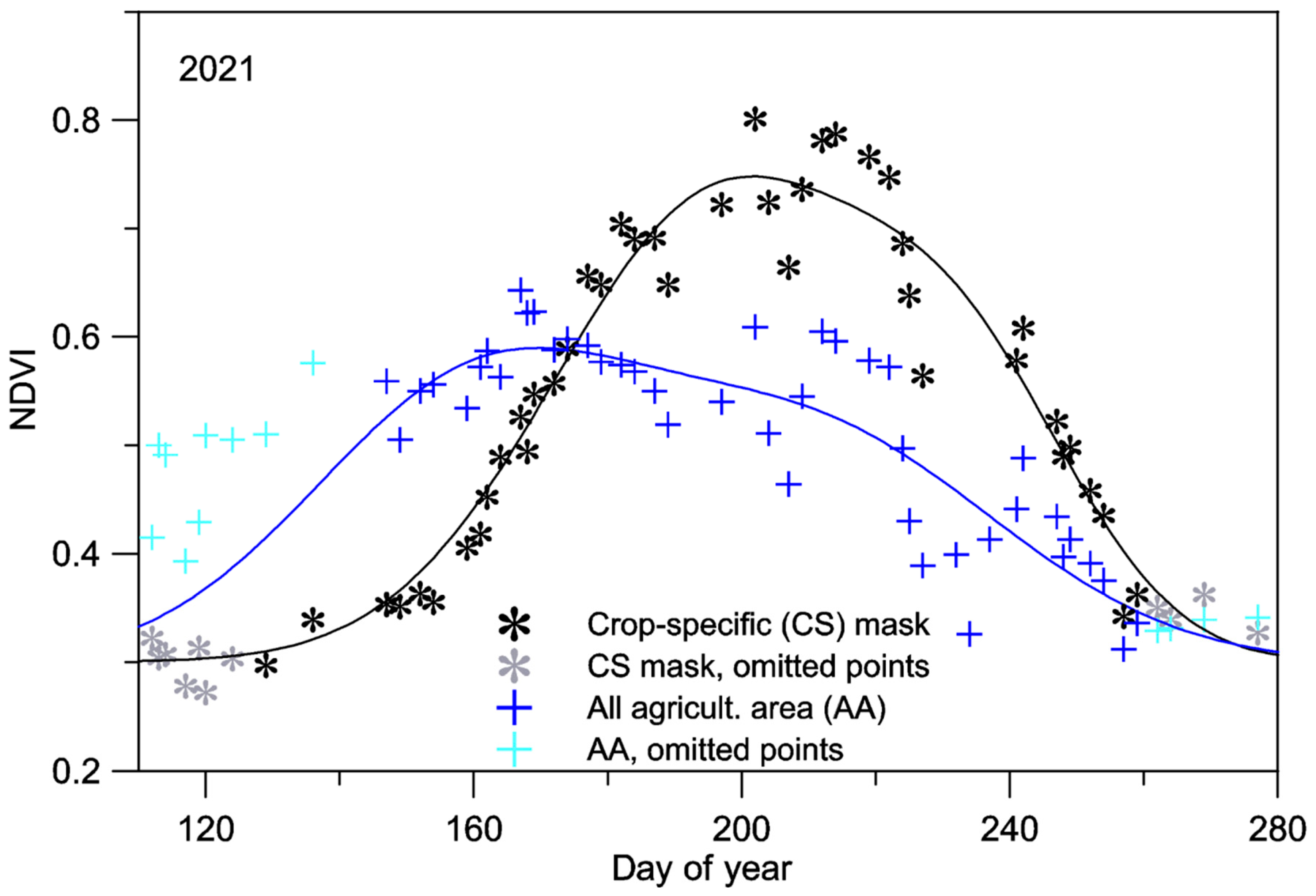
Figure 7.
GYURRI (General Yield Robust Reference Index) – yield (a) and GYURI (General Yield Reference Index) – yield (b) data with the lines fitted by the least square method. (R-D: robust diagnostic; CS-D: crop-specific diagnostic.).
Figure 7.
GYURRI (General Yield Robust Reference Index) – yield (a) and GYURI (General Yield Reference Index) – yield (b) data with the lines fitted by the least square method. (R-D: robust diagnostic; CS-D: crop-specific diagnostic.).
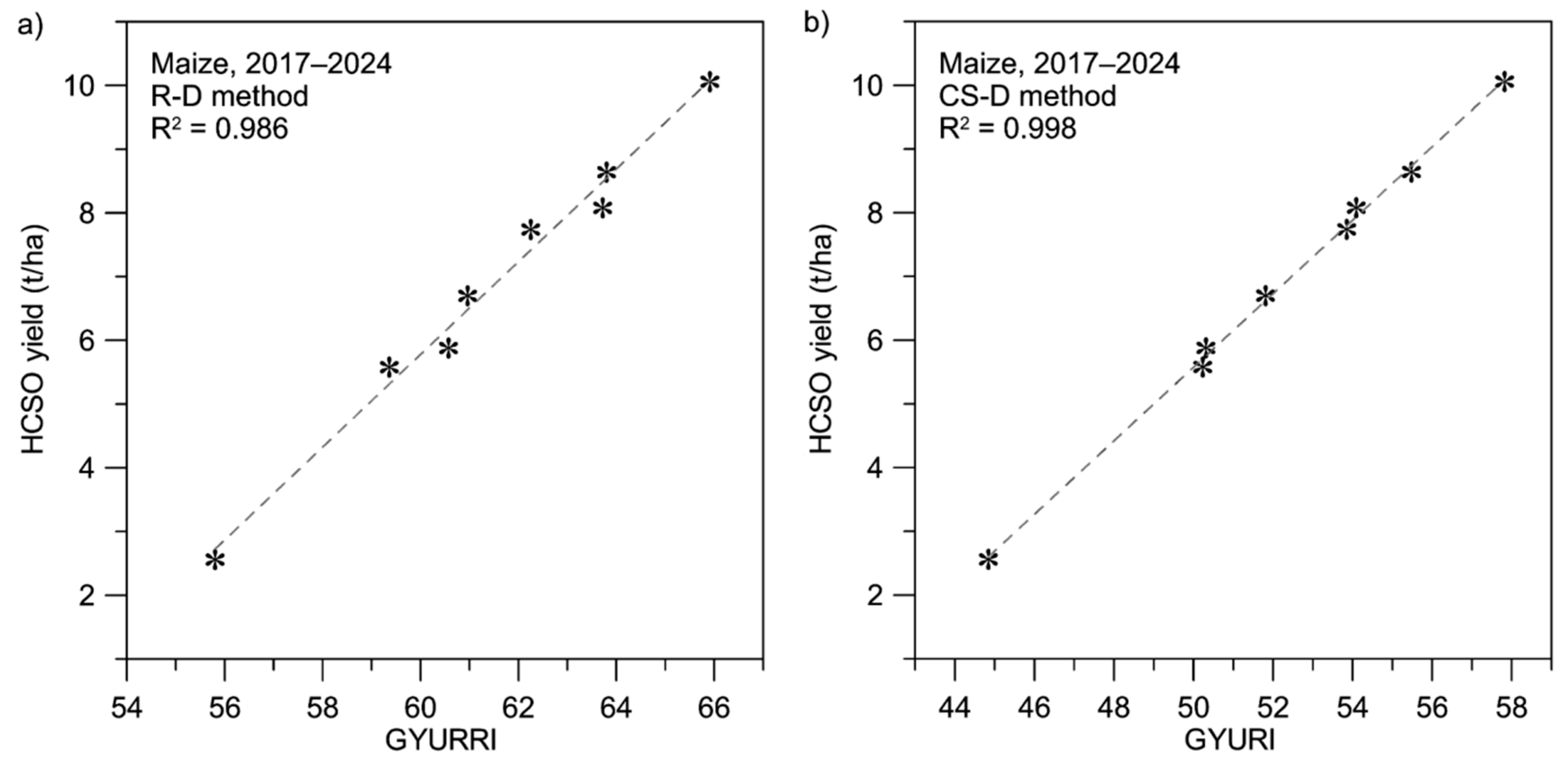
Figure 8.
The estimated yield data obtained from the R-P (robust predictive) and CS-P (crop-specific predictive) models.
Figure 8.
The estimated yield data obtained from the R-P (robust predictive) and CS-P (crop-specific predictive) models.
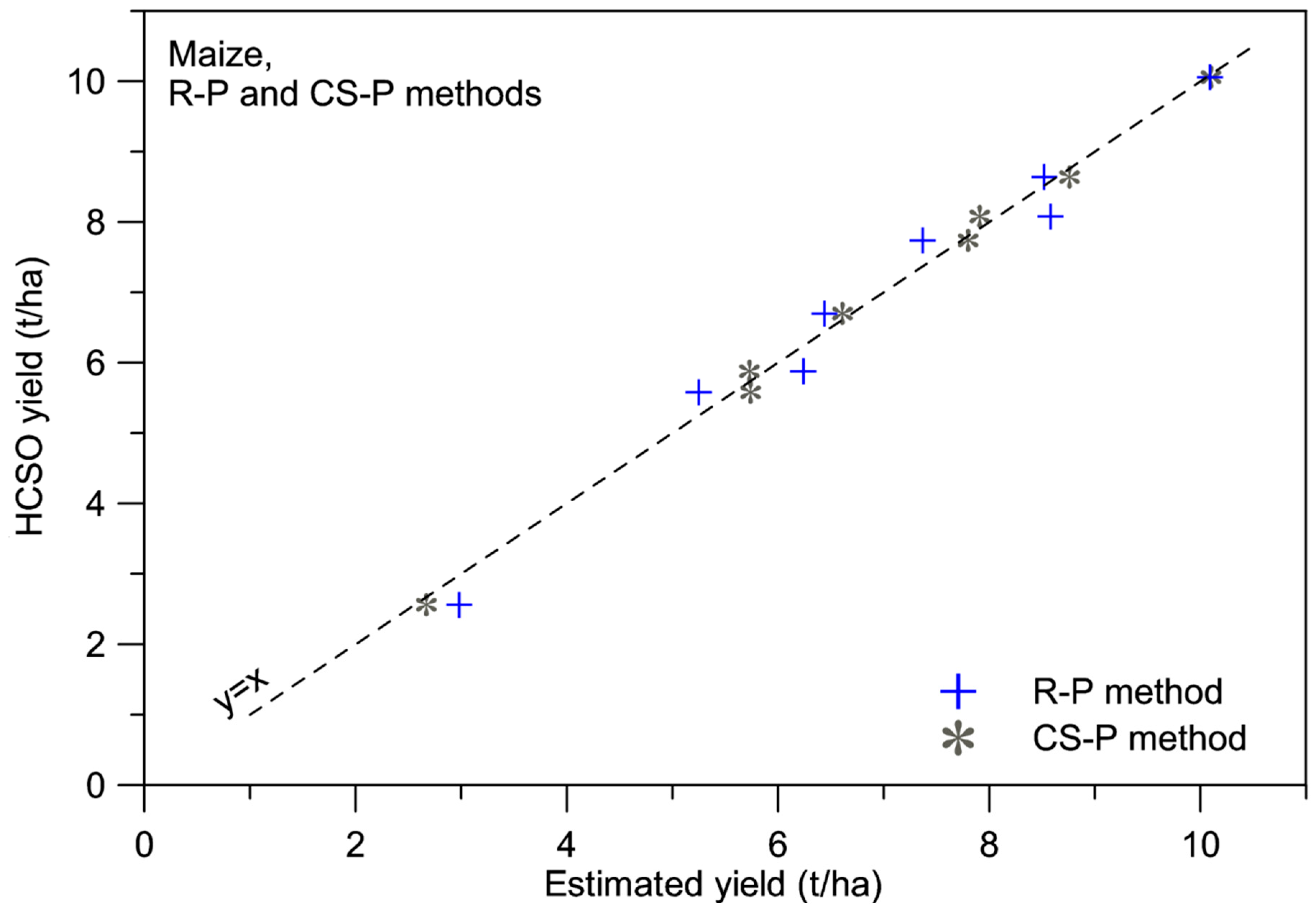
Figure 9.
HCSO official yield data and estimated yields of the four models for maize.
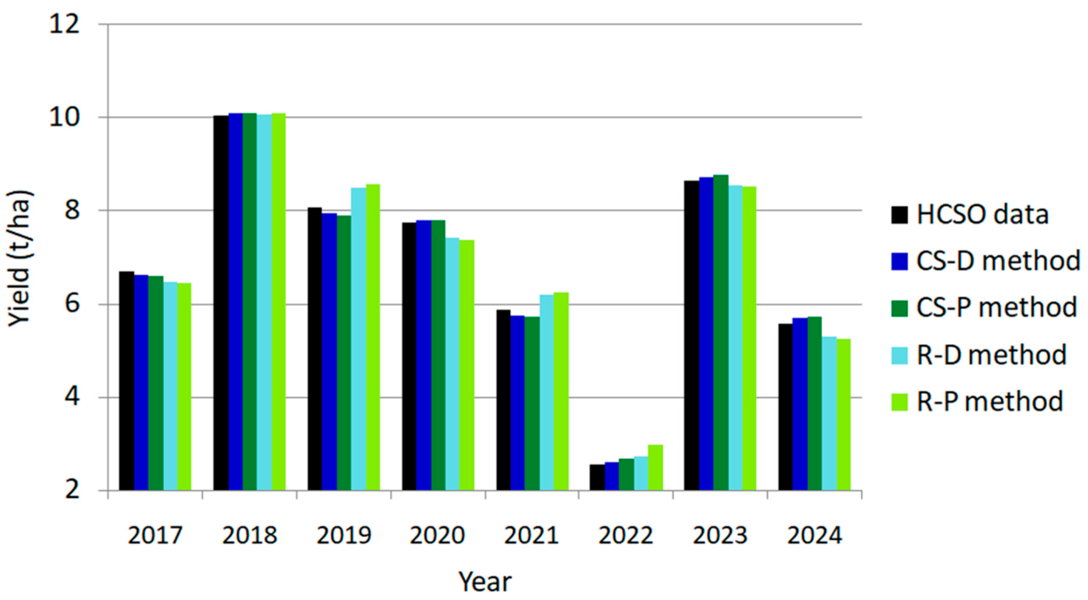
Figure 10.
Estimation results of the quasi-operative procedure (based on years 2017–2021) and the CS-P model (based on 2017–2021, 2023 and 2024) for 2022.
Figure 10.
Estimation results of the quasi-operative procedure (based on years 2017–2021) and the CS-P model (based on 2017–2021, 2023 and 2024) for 2022.
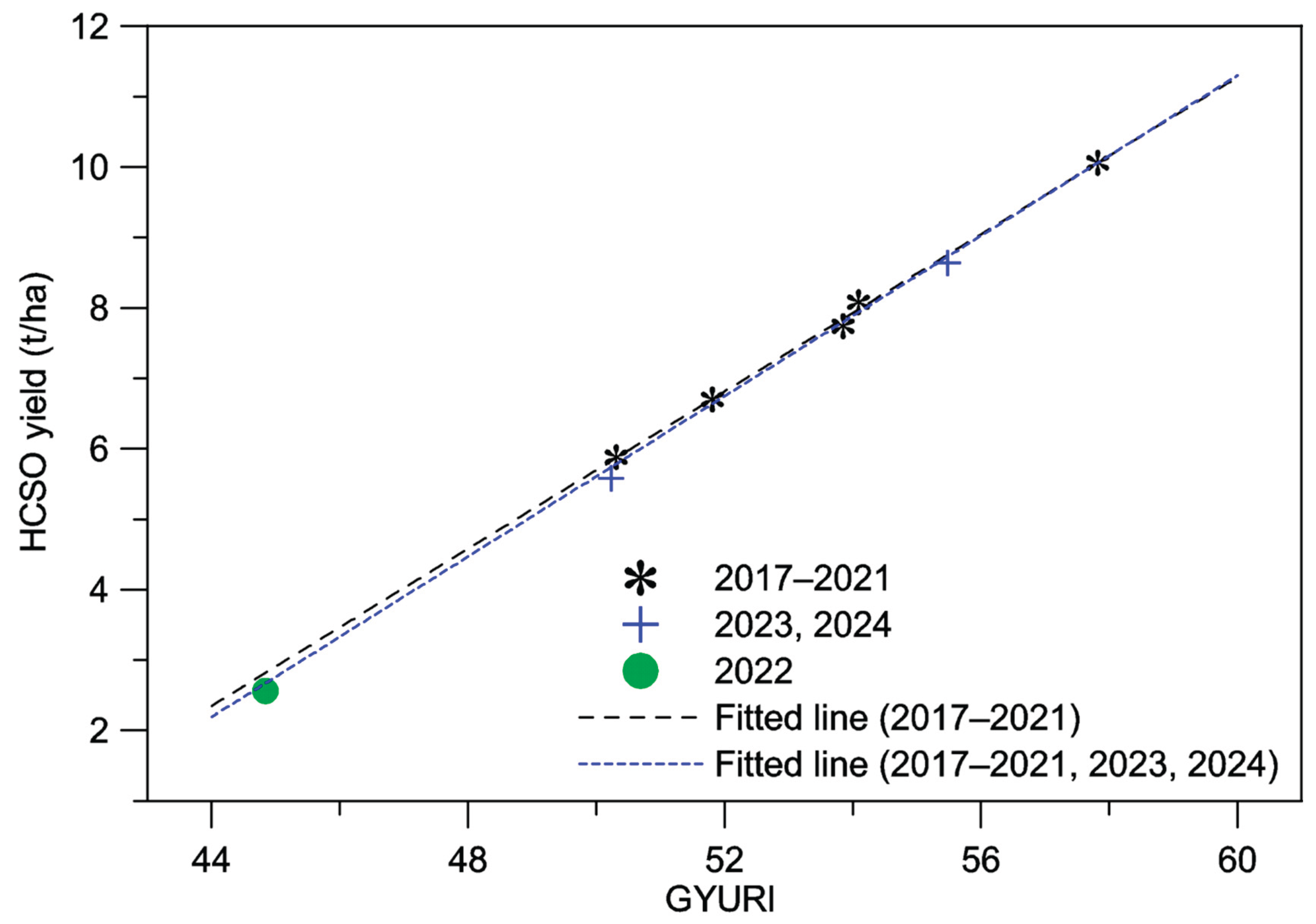
Figure 11.
Correlation coefficients in the CS-D model for maize using different te values.
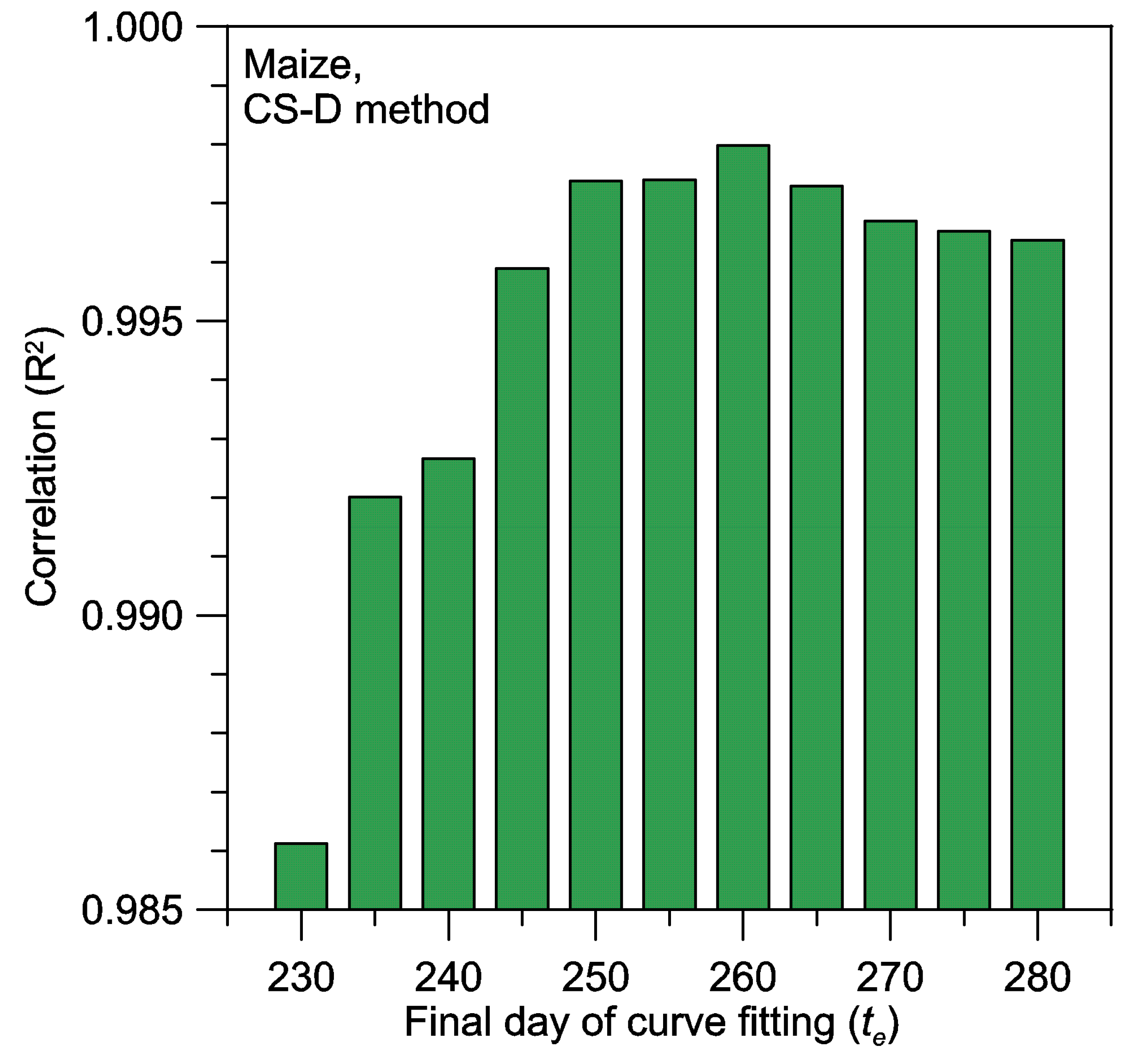
Figure 12.
The obtained MAPE (Mean Absolute Percentage Error) values using the R-P and CS-P models at different forecast dates.
Figure 12.
The obtained MAPE (Mean Absolute Percentage Error) values using the R-P and CS-P models at different forecast dates.
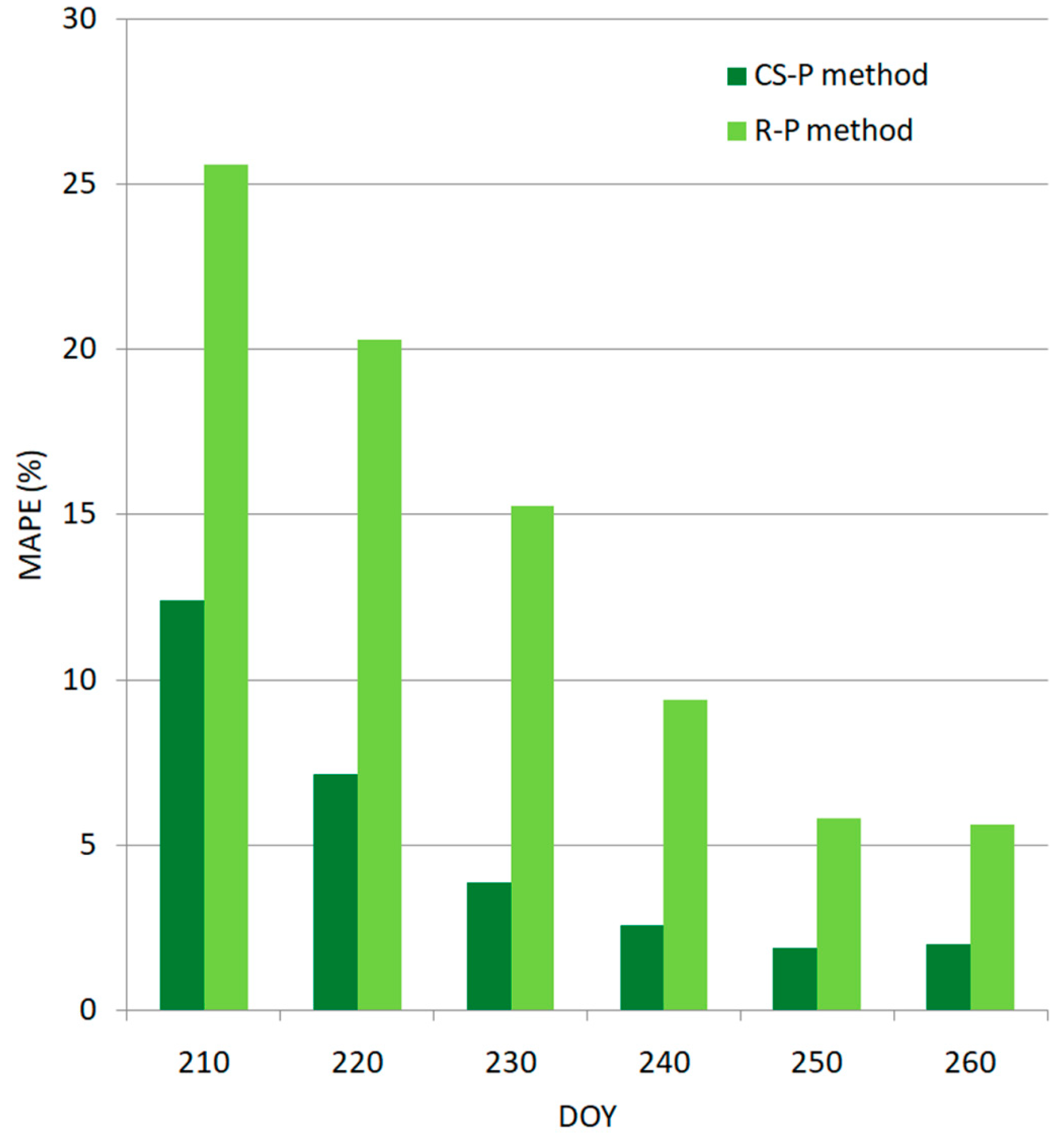
Figure 13.
The NDVI time-series for maize and sunflower fields in 2020.
Figure 14.
Correlation coefficients in the CS-D model for sunflower using different te values.
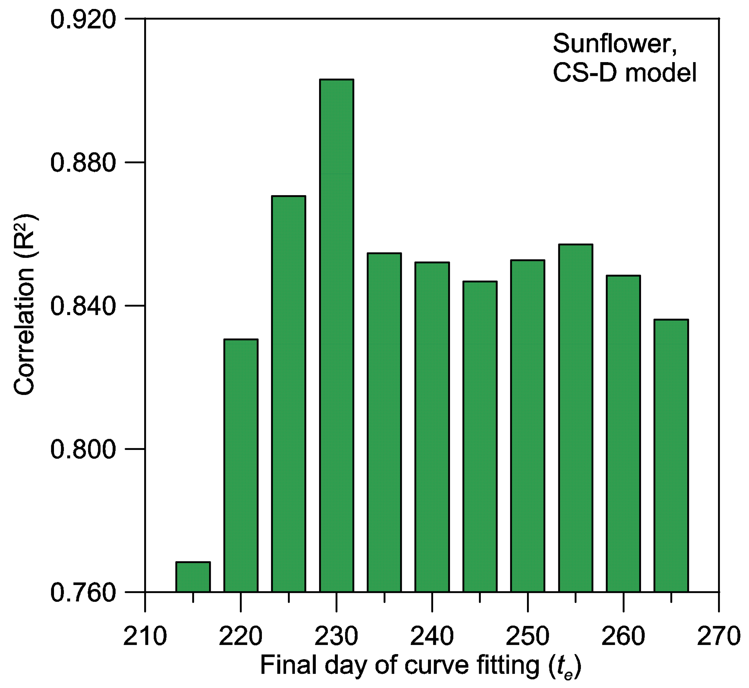
Figure 15.
Results of yield estimation models for sunflower.
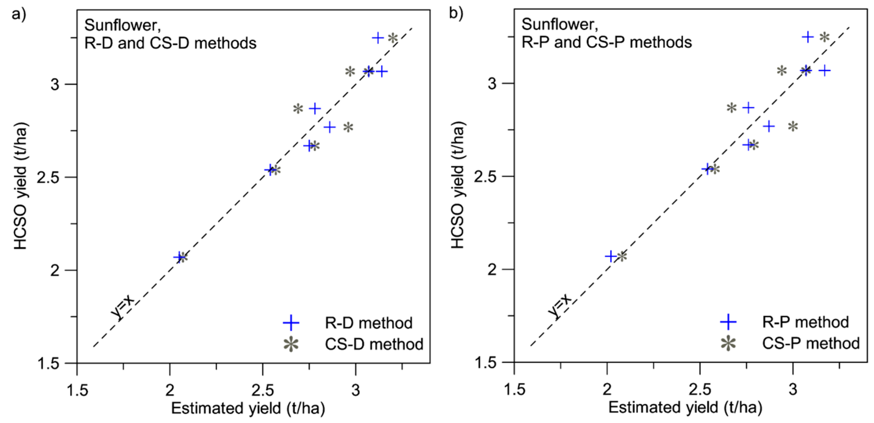
Figure 16.
HCSO official yield data and estimated yields of the four models for sunflower.
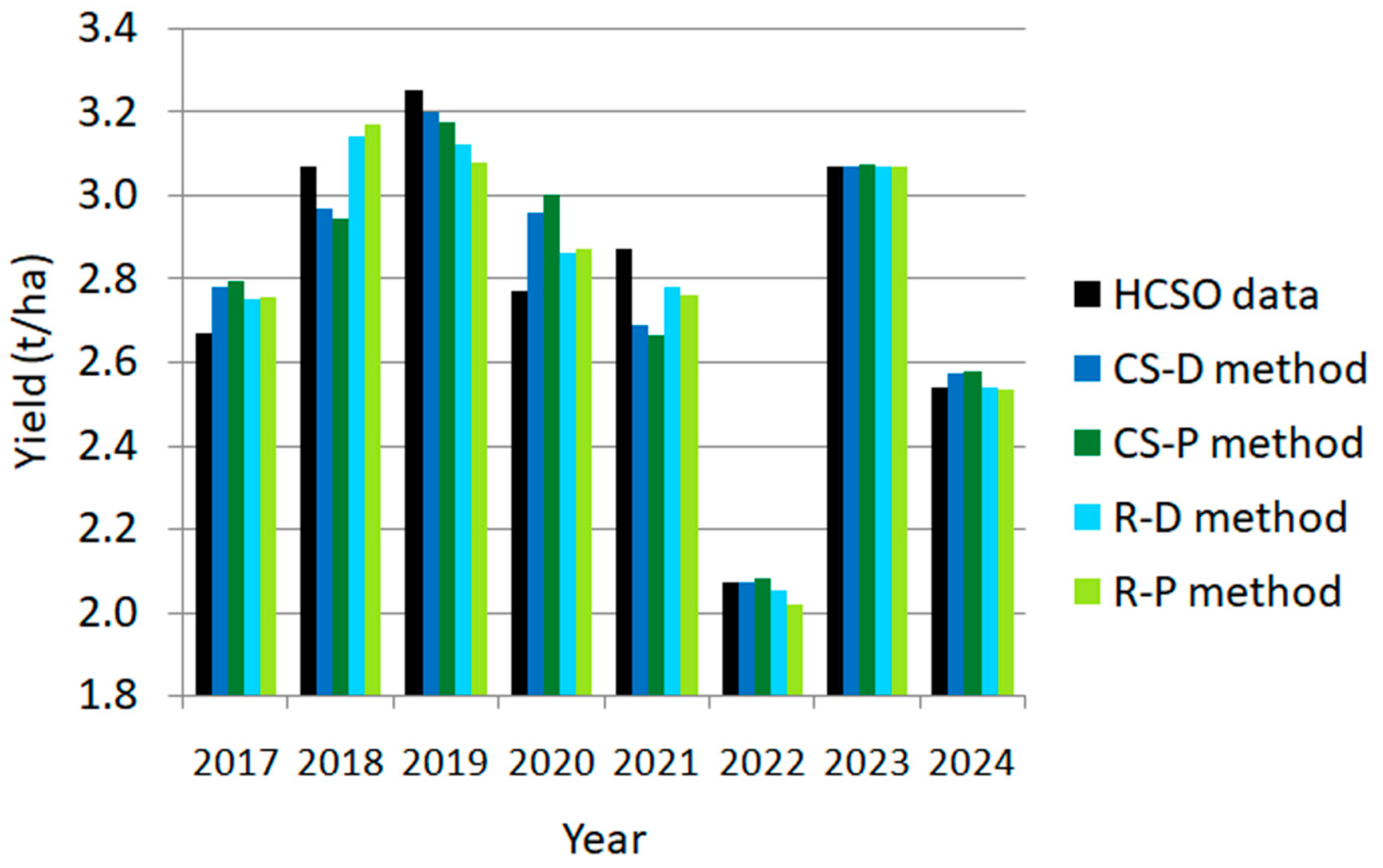

Table 1.
Differences between estimated and HCSO (Hungarian Central Statistical Office) yield data for maize using the R-D (robust diagnostic) and CS-D (crop-specific diagnostic) methods.
Table 1.
Differences between estimated and HCSO (Hungarian Central Statistical Office) yield data for maize using the R-D (robust diagnostic) and CS-D (crop-specific diagnostic) methods.
| Year |
Estimated yield (t/ha) |
HCSO yield (t/ha) |
Estimated - HCSO (t/ha) |
Estimated - HCSO (%) |
|||
| R-D | CS-D | R-D | CS-D | R-D | CS-D | ||
| 2017 | 6.48 | 6.62 | 6.70 | –0.22 | –0.08 | –3.28 | –1.19 |
| 2018 | 10.08 | 10.09 | 10.06 | 0.02 | 0.03 | 1.63 | 0.30 |
| 2019 | 8.49 | 7.94 | 8.08 | 0.41 | –0.14 | 5.07 | –1.73 |
| 2020 | 7.42 | 7.80 | 7.74 | –0.32 | 0.06 | –4.13 | 0.78 |
| 2021 | 6.19 | 5.76 | 5.88 | 0.31 | –0.12 | 5.27 | –2.04 |
| 2022 | 2.72 | 2.60 | 2.56 | 0.16 | 0.04 | 6.25 | 1.56 |
| 2023 | 8.54 | 8.73 | 8.64 | –0.10 | 0.09 | –1.16 | 1.04 |
| 2024 | 5.31 | 5.71 | 5.58 | –0.27 | 0.13 | –4.84 | 2.33 |
| Average absolute differences: | 0.23 | 0.09 | 3.78 | 1.37 | |||
Table 2.
Differences between estimated and HCSO yield data for maize using the R-P (robust predictive) and CS-P (crop-specific predictive) methods.
Table 2.
Differences between estimated and HCSO yield data for maize using the R-P (robust predictive) and CS-P (crop-specific predictive) methods.
| Year |
Estimated yield (t/ha) |
HCSO yield (t/ha) |
Estimated - HCSO (t/ha) |
Estimated - HCSO (%) |
|||
| R-P | CS-P | R-P | CS-P | R-P | CS-P | ||
| 2017 | 6.44 | 6.61 | 6.70 | –0.26 | –0.09 | –3.84 | –1.38 |
| 2018 | 10.09 | 10.10 | 10.06 | 0.03 | 0.04 | 0.31 | 0.44 |
| 2019 | 8.58 | 7.91 | 8.08 | 0.50 | –0.17 | 6.22 | –2.10 |
| 2020 | 7.37 | 7.80 | 7.74 | –0.37 | 0.06 | –4.79 | 0.83 |
| 2021 | 6.24 | 5.73 | 5.88 | 0.36 | –0.15 | 6.17 | –2.55 |
| 2022 | 2.98 | 2.67 | 2.56 | 0.42 | 0.11 | 16.35 | 4.42 |
| 2023 | 8.52 | 8.76 | 8.64 | –0.12 | 0.12 | –1.37 | 1.44 |
| 2024 | 5.58 | 5.74 | 5.58 | –0.33 | 0.16 | –5.93 | 2.81 |
| Average absolute differences: | 0.30 | 0.11 | 5.62 | 2.00 | |||
Table 3.
Result of the quasi-operative yield estimation method for maize using the CS-P model.
|
Year of estimation |
Years used to build the model |
Fitted parameters Yield=a*GYURI+b |
GYURI |
Estimated yield (t/ha) |
HCSO yield (t/ha) |
Estimated - HCSO | ||
| a | b | (t/ha) | (%) | |||||
| 2020 | 2017–19 | 0.5557 | –22.0479 | 53.85 | 7.88 | 7.74 | 0.14 | 1.76 |
| 2021 | 2017–20 | 0.5597 | –22.2977 | 50.31 | 5.87 | 5.88 | –0.02 | –0.33 |
| 2022 | 2017–21 | 0.5573 | –22.1678 | 44.84 | 2.82 | 2.56 | 0.26 | 10.22 |
| 2023 | 2017–22 | 0.5771 | –23.2426 | 55.48 | 8.78 | 8.64 | 0.13 | 1.56 |
| 2024 | 2017–23 | 0.5735 | –23.0699 | 50.23 | 5.74 | 5.58 | 0.16 | 2.81 |
GYURI: General Yield Reference Index.
Table 4.
Result of forecast for maize using the CS-P model.
| Year |
HCSO yield (t/ha) |
Forecast on DOY=250 |
Forecast on DOY=240 |
Forecast on DOY=230 |
|||
|
Yield (t/ha) |
Diff. (%) |
Yield (t/ha) |
Diff. (%) |
Yield (t/ha) |
Diff. (%) |
||
| 2017 | 6.70 | 6.60 | –1.55 | 6.57 | –1.90 | 6.58 | –1.73 |
| 2018 | 10.06 | 10.02 | –0.37 | 10.05 | –0.14 | 10.19 | 1.30 |
| 2019 | 8.08 | 8.05 | –0.33 | 8.32 | 3.01 | 8.58 | 6.20 |
| 2020 | 7.74 | 7.82 | 0.98 | 7.82 | 0.98 | 7.50 | –3.13 |
| 2021 | 5.88 | 5.66 | –3.83 | 5.48 | –6.78 | 5.48 | –6.78 |
| 2022 | 2.56 | 2.66 | 3.75 | 2.59 | 1.09 | 2.50 | –2.47 |
| 2023 | 8.64 | 8.75 | 1.24 | 8.98 | 3.93 | 9.05 | 4.80 |
| 2024 | 5.58 | 5.74 | 2.92 | 5.72 | 2.51 | 5.83 | 4.46 |
| Average absolute difference: | 1.87 | 2.54 | 3.86 | ||||
Diff.: Difference.
Table 5.
Differences between estimated and HCSO yield data for sunflower using the R-D and CS-D methods.
Table 5.
Differences between estimated and HCSO yield data for sunflower using the R-D and CS-D methods.
| Year |
Estimated yield (t/ha) |
HCSO yield (t/ha) |
Estimated - HCSO (t/ha) |
Estimated - HCSO (%) |
|||
| R-D | CS-D | R-D | CS-D | R-D | CS-D | ||
| 2017 | 2.75 | 2.78 | 2.67 | 0.08 | 0.11 | 3.00 | 4.12 |
| 2018 | 3.14 | 2.97 | 3.07 | 0.07 | –0.10 | 2.28 | –3.26 |
| 2019 | 3.12 | 3.20 | 3.25 | –0.13 | –0.05 | –4.00 | –1.54 |
| 2020 | 2.86 | 2.96 | 2.77 | 0.09 | 0.19 | 3.25 | 6.86 |
| 2021 | 2.78 | 2.69 | 2.87 | –0.09 | –0.18 | –3.14 | –6.27 |
| 2022 | 2.05 | 2.07 | 2.07 | –0.02 | 0.00 | –0.97 | 0.00 |
| 2023 | 3.07 | 3.07 | 3.07 | 0.00 | 0.00 | 0.00 | 0.00 |
| 2024 | 2.54 | 2.57 | 2.54 | 0.00 | 0.03 | 0.00 | 1.18 |
| Average absolute differences: | 0.06 | 0.08 | 2.08 | 2.90 | |||
Table 6.
Differences between estimated and HCSO yield data for sunflower using the R-P and CS-P methods.
Table 6.
Differences between estimated and HCSO yield data for sunflower using the R-P and CS-P methods.
| Year |
Estimated yield (t/ha) |
HCSO yield (t/ha) |
Estimated - HCSO (t/ha) |
Estimated - HCSO (%) |
|||
| R-P | CS-P | R-P | CS-P | R-P | CS-P | ||
| 2017 | 2.67 | 2.79 | 2.67 | 0.09 | 0.12 | 3.23 | 4.68 |
| 2018 | 3.17 | 2.94 | 3.07 | 0.10 | –0.13 | 3.26 | –4.09 |
| 2019 | 3.08 | 3.17 | 3.25 | –0.17 | –0.08 | –5.23 | –2.23 |
| 2020 | 2.87 | 3.00 | 2.77 | 0.10 | 0.23 | 3.63 | 8.27 |
| 2021 | 2.76 | 2.67 | 2.87 | –0.11 | –0.20 | –3.76 | –7.14 |
| 2022 | 2.02 | 2.08 | 2.07 | –0.05 | 0.01 | –2.52 | 0.50 |
| 2023 | 3.07 | 3.07 | 3.07 | –0.00 | 0.00 | –0.09 | 0.13 |
| 2024 | 2.54 | 2.58 | 2.54 | –0.00 | 0.04 | –0.16 | 1.52 |
| Average absolute differences: | 0.08 | 0.10 | 2.73 | 3.58 | |||
Table 7.
Result of quasi-operative yield estimation method for sunflower using the CS-P model.
|
Year of estimation |
Years used to build the model |
Fitted parameters Yield=a*GYURI+b |
GYURI |
Estimated yield (t/ha) |
HCSO yield (t/ha) |
Estimated - HCSO | ||
| a | b | (t/ha) | (%) | |||||
| 2020 | 2017-19 | 0.1366 | –3.2413 | 44.33 | 2.81 | 2.77 | 0.04 | 1.59 |
| 2021 | 2017-20 | 0.1413 | –3.4665 | 43.58 | 2.69 | 2.87 | –0.18 | –6.22 |
| 2022 | 2017-21 | 0.1209 | –2.5101 | 36.99 | 1.96 | 2.07 | –0.11 | –5.22 |
| 2023 | 2017-22 | 0.1097 | –2.0026 | 46.25 | 3.07 | 3.07 | 0.00 | 0.00 |
| 2024 | 2017-23 | 0.1097 | –2.0046 | 41.39 | 5.54 | 2.54 | 0.00 | 0.00 |
Table 8.
Statistical results of the four models.
| Model | Maize | Sunflower | |||||||||
| te | R2 | MAE (t/ha) |
RMSE (t/ha) |
MAPE (%) | te | R2 |
MAE (t/ha) |
RMSE (t/ha) |
MAPE (%) | ||
| R-D | 260 | 0.9857 | 0.226 | 0.256 | 3.78 | 230 | 0.9538 | 0.060 | 0.075 | 2.08 | |
| CS-D | 260 | 0.9981 | 0.086 | 0.095 | 1.37 | 230 | 0.9031 | 0.083 | 0.108 | 2.90 | |
| R-P | 260 | 0.9759 | 0.299 | 0.333 | 5.62 | 230 | 0.9276 | 0.078 | 0.094 | 2.73 | |
| CS-P | 260 | 0.9968 | 0.114 | 0.121 | 2.00 | 230 | 0.8637 | 0.102 | 0.129 | 3.58 | |
| R-P | 250 | 0.9778 | 0.296 | 0.320 | 5.82 | 220 | 0.6542 | 0.123 | 0.205 | 4.08 | |
| R-P | 240 | 0.9161 | 0.527 | 0.621 | 9.40 | 210 | 0.3192 | 0.293 | 0.364 | 9.90 | |
| R-P | 230 | 0.7308 | 0.951 | 1.112 | 15.26 | - | |||||
| CS-P | 250 | 0.9968 | 0.104 | 0.121 | 1.87 | 220 | 0.7939 | 0.128 | 0.158 | 4.40 | |
| CS-P | 240 | 0.9898 | 0.171 | 0.217 | 2.54 | 210 | 0.4074 | 0.215 | 0.268 | 7.22 | |
| CS-P | 230 | 0.9800 | 0.264 | 0.304 | 3.86 | - | |||||
| CS-P | 220 | 0.9231 | 0.500 | 0.595 | 7.14 | - | |||||
R2: Correlation coefficient; MAE: Mean Absolute Error; RMSE: Root Mean Square Error; MAPE: Mean Absolute Percentage Error; te : End day of curve-fitting.
Disclaimer/Publisher’s Note: The statements, opinions and data contained in all publications are solely those of the individual author(s) and contributor(s) and not of MDPI and/or the editor(s). MDPI and/or the editor(s) disclaim responsibility for any injury to people or property resulting from any ideas, methods, instructions or products referred to in the content. |
© 2025 by the authors. Licensee MDPI, Basel, Switzerland. This article is an open access article distributed under the terms and conditions of the Creative Commons Attribution (CC BY) license (http://creativecommons.org/licenses/by/4.0/).
Copyright: This open access article is published under a Creative Commons CC BY 4.0 license, which permit the free download, distribution, and reuse, provided that the author and preprint are cited in any reuse.


