
Submitted:
02 December 2025
Posted:
05 December 2025
You are already at the latest version
Abstract
Difficult access and a lack of in situ data limit monitoring of high-Andean wetlands, which are key components of water regulation in central Chile. This study analyzes the multitemporal dynamics of vegetation in three high Andean wetlands of the headwater (1HW), lateral (2LW), and confluence (3CW) types in the Los Nogales Nature Sanctuary between 2018 and 2025. We integrated Sentinel-2 Level 2A images, annual accumulated precipitation from the ERA5-Land product (lag-1 year), and high-resolution UAV-derived boundaries to characterize six spectral indices (NDVI, EVI, NDRE704, NDRE705, NDWI, and SAVI) and their relationship with water variability.
Annual precipitation ranged from ~420 to 780 mm during a regional megadrought. The headwater wetland showed the greatest climate sensitivity, with significant correlations between the previous year's precipitation and NDVI, NDRE705, EVI, SAVI, and NDWI (|R| ≥ 0.70; p < 0.05), while in the lateral and confluence wetlands, the relationships were moderate or weak. Multitemporal mosaics showed maximum vegetative vigor between 2018 and 2021, followed by a decline. Overall, the results confirm that integrating the Sentinel-2 series, climate reanalysis, and UAV delimitation is an effective tool for ecohydrological monitoring and management of high-Andean wetlands.
Keywords:
Sentinel-2
; ERA5-Land
; high-Andean wetlands
; UAV
1. Introduction
The sustained increase in greenhouse gas emissions has raised the global average temperature by 1.55 ± 0.13 °C above pre-industrial levels, intensifying the occurrence of extreme weather events and altering the dynamics of highly vulnerable ecosystems [1,2]. Among these, high-Andean wetlands stand out for their role in water regulation, carbon storage, and providing habitat for endemic and migratory species [3,4]. In Chile, these ecosystems are mainly distributed above 3000 meters above sea level, in mountainous environments in the north, center, and south of the country, taking various forms such as meadows, bogs, peat bogs, and salt flats [5].
These wetlands are highly hydroecologically sensitive due to their location in mountainous areas, where water availability depends heavily on winter precipitation and snowmelt [5]. This dependence makes them particularly susceptible to both climatic and anthropogenic disturbances. Added to this are pressures such as grazing, water extraction, and mining activities, which affect their hydrological and vegetational functioning [6,7]. Since 2010, the megadrought affecting central Chile has intensified this vulnerability, leading to sustained reductions in precipitation and altering the structure and productivity of vegetation [8,9].
Continuous monitoring of these ecosystems faces difficulties associated with their size, the complexity of access, and the scarcity of long-term hydrometeorological series [6,7]. In this context, satellite remote sensing has established itself as an efficient tool for characterizing vegetation dynamics using spectral indicators derived from multitemporal images [10]. Among the most widely used indices are EVI, NDRE704, NDRE705, NDVI, NDWI, and SAVI, which capture different dimensions of vegetation’s ecological response. EVI is sensitive to variations in biomass and vegetation cover structure; NDRE reflects changes in chlorophyll content and leaf stress; NDVI represents vegetation productivity and vigor; NDWI is related to foliage and surface soil moisture; and SAVI corrects for the effect of soil background in areas of low cover [11,12,13,14,15,16,17].
Several studies have shown that the magnitude and seasonality of precipitation directly influence vegetation cover, particularly in semi-arid and mountain environments [18,19,20]. Globally, research conducted in the Chilean-Bolivian highlands, the Salar de Huasco, and the Cordillera Blanca (Peru) has used remote sensing to characterize vegetation response to climate variability and environmental gradients [21,22,23,24,25]. However, in central Chile, studies that integrate multitemporal series of spectral indicators such as EVI, NDRE704, NDRE705, NDVI, NDWI, and SAVI remain scarce. In particular, wetlands located in the transition zones of the mountain range in the Metropolitan Region have limited research coverage and limited availability of systematic information, despite their relevance to regional water regulation [5]. This lack of specific studies underscores the need to evaluate their dynamics using spectral indicators derived from remote sensing.
Over the last decade, the use of extensive time series and machine learning techniques has improved the detection of vegetation changes and the spatial characterization of wetlands [26,27]. These methodologies, which integrate multiple spectral indicators, have proven effective for analyzing the dynamics and functioning of ecosystems with high climatic and spatial variability [26]. Their application in high-Andean wetlands provides a solid methodological basis for evaluating changes in vegetation cover and responses to variations in the water regime, which are essential for addressing the objective of this study [21,22,23,24,25].
In this context, the present study evaluates the multitemporal dynamics of vegetation in three high-Andean wetlands within the Los Nogales Nature Sanctuary, representative of the functional types of headwaters, laterals, and confluences, during the period 2018–2025. The analysis uses spectral indicators derived from Sentinel-2 images and supplements them with annual accumulated precipitation data from the ERA5-Land product. Multispectral drone flights delimited the wetlands.
The main objective is to identify which spectral indicator shows the most consistent relationship with the accumulated precipitation of the previous year, as well as to determine which functional type of wetland exhibits greater sensitivity to variations in the water regime.
2. Materials and Methods
2.1. Study Area
The Los Nogales Nature Sanctuary (SNLN) lies in the Metropolitan Region of Chile, between coordinates 33°19′46.441″ S; 70°26′52.526″ W and 33°6′19.015″ S; 70°20′52.037″ W (Figure 1).
In the northwestern sector of the sanctuary, a system of approximately eight high-Andean wetlands is distributed altitudinally from the highest part of the basin to the middle and lower areas, forming an ecohydrological gradient associated with variations in slope, humidity, and water supply.
Within this system, we identify three wetlands representative of the main functional types of the ecosystem: headwater wetland (1HW), lateral wetland (2LW), and confluence wetland (3CW). These three wetlands differ in their position on the altitudinal gradient and in their characteristic hydrological conditions.
The surfaces of each wetland are presented in Table 1, with values of 9.17 ha for the headwater wetland, 8.18 ha for the lateral wetland, and 2.14 ha for the confluence wetland, for a total of 19.49 ha. Figure 1 shows the location of the SNLN within the regional context and the spatial distribution of the three analyzed wetlands. The base map uses a satellite image from Maxar (2022), while flights conducted with a multispectral drone provided the precise delimitation of the wetlands.
2.2. Methodology
To evaluate the relationship between vegetation and precipitation in the three high-Andean wetlands of the SNLN, the methodological flow shown in Figure 2 was applied. This procedure integrated climate data, satellite imagery, and UAV-derived photogrammetric products.
We used three primary sources of information:
- (i)
- Climate data from the ERA5-Land product (2017–2025)
- (ii)
- Sentinel-2 Level 2A images (2018–2025).
- (iii)
- UAV flights for the precise delimitation of wetlands (carried out on 2 February 2025)
The ERA5-Land data, obtained from Google Earth Engine (GEE), have a spatial resolution of 0.1° (~9 km) and a monthly temporal resolution. Based on these data, we calculated the annual accumulated precipitation (lag-1 year), following methodologies applied in ecohydrological studies of semi-arid and high Andean areas [7,8,31].
The spectral indices EVI, NDRE704, NDRE705, NDVI, NDWI, and SAVI were generated in GEE using Sentinel-2 Level 2A images (10 m, 5-day revisit), selected under a cloud cover threshold of <10%. Masking was applied using the Scene Classification Layer (SCL) to remove pixels with clouds, shadows, and cirrus clouds [32]. For each wetland, we extracted the average value of each index within the polygon, yielding a monthly time series from 2018 to 2025.
We conducted the UAV flights on February 2, 2025, and processed the data in Site Scan for ArcGIS [35] to generate RGB orthomosaics with resolutions of 2–5 cm. We used these products to accurately delimit the wetlands.
Finally, we performed a Pearson correlation analysis between the cumulative annual precipitation of the previous year and the average summer (December–February) values of each spectral index. We selected this coefficient because studies evaluating linear relationships between climate variables and vegetation spectral responses have used it [38].
2.3. Climatic Data
We obtained climate data from the ERA5-Land reanalysis dataset, developed by the European Center for Medium-Range Weather Forecasts (ECMWF). This product provides high spatial and temporal resolution information, optimized for the analysis of land surface variables [31].
We extracted total precipitation (rain + snow) from the Total Precipitation (tp) band, initially expressed in meters per unit of time, and subsequently converted it to monthly millimeters. We used data from January 2017 to September 2025 to analyze the influence of the previous year’s accumulated precipitation (PPc) on vegetation development the following year.
The ERA5-Land Monthly Aggregated product has a spatial resolution of 0.1° (~9 km) and a monthly temporal resolution, enabling it to capture interannual climate variability in mountain ecohydrological studies accurately.
Scripts developed in Google Earth Engine (GEE) [32] generated the monthly and annual series using the ECMWF/ERA5_LAND/MONTHLY_AGGR collection. The data were then exported and processed in RStudio (v4.3.3) to calculate the PPc and organize the time series.
We used a 1-year time lag between precipitation and vegetation indices to evaluate the delayed response of vegetation to water availability, following methodologies applied in semi-arid and high-Andean ecosystems in Chile [7,8].
2.4. Vegetation Indices Derived of Sentinel-2 and UAV Data
We calculated six spectral indices derived from Sentinel-2 Level 2A images spanning January 2018 to September 2025 to characterize the seasonal and interannual variability of vegetation in high Andean wetlands. The indices included were NDVI, EVI, NDRE704, NDRE705, NDWI, and SAVI, selected for their established use in vegetation monitoring and for representing complementary dimensions related to vigor, chlorophyll content, vegetation cover moisture, and soil background effects [10,11,12,13,14,15,16,17].
Table 2 presents the equations, bands used, uses, and corresponding references for each index:
For each available date, we calculated the index values within the polygon of each wetland. When a wetland had multiple polygons or internal subdivisions, the final value used was the average index within each polygon or subdivision to obtain a representative time series for the wetland. This approach is standard in vegetation studies based on optical sensors when the objective is to characterize temporal trends at the patch or ecosystem scale [21,22,23]. We subsequently used these series to identify the maximum annual values and to calculate the summer averages used in the statistical analyses.
We calculated the Sentinel-2-derived indices using scripts in Google Earth Engine (GEE) [32], using only Level 2A images with cloud cover <10%. For preprocessing, we applied atmospheric masking based on the Scene Classification Layer (SCL), removing pixels classified as clouds, shadows, or cirrus clouds.
2.5. Statistical Analysis
Statistical analysis was performed in R (v4.3.2) using RStudio as the integrated development environment [36,37]. We used the dplyr, tidyr, lubridate, ggplot2, Metrics and purrr libraries for data processing and visualization.
The objective of the analysis was to quantify the linear relationship between the cumulative annual precipitation of the previous year (lag-1) and the average summer (December–February) values of the vegetation indices for each wetland and spectral indicator.
We imported the files derived from the EVI, NDRE704, NDRE705, NDVI, NDWI, and SAVI indices from specific directories for each wetland functional type (headwaters, lateral, and confluence). We standardized each file to contain the variables date, index, wetland, and value. We homogenized the dates using a robust parsing function to ensure compatibility between different formats.
For each year, we calculated summer averages by grouping the months of December, January, and February. The month of December was assigned to the following year, generating the temporal variable summer_year, which represents each summer season.
The cumulative annual precipitation (PPc), obtained from the ERA5-Land product, was calculated considering a time lag of one year (lag-1), comparing the PPc of year Y–1 with the vegetation response in the summer of year Y. This approach has been previously applied in studies analyzing delayed ecological reactions to variations in water availability in semi-arid and high-Andean systems [7,8].
We evaluated the relationship between precipitation and spectral indices using Pearson’s correlation coefficient (r), widely used in ecological and remote sensing studies to measure the strength and direction of linear relationships between biophysical indicators and climate variables [38]. For each wetland–index combination, the following statistical metrics were calculated [39,40,41]:
- R: Pearson correlation coefficient.
- R²: coefficient of determination.
- RMSE (Root Mean Square Error) and MAE (Mean Absolute Error): indicators of model fitting error.
- p-value: level of statistical significance.
Linear models (lm(y ~ x)) were fitted for each wetland case, generating scatter plots with regression lines and statistical results.
We present the equations and interpretations for each metric in Table 3.
2.6. UAV Photogrammetry
Before the flights, we conducted a terrain survey to verify access, topographic conditions, and the location of each wetland. On this basis, we conducted photogrammetric flights with a DJI Mavic 3 Multispectral UAV (DJI, Shenzhen, China), equipped with a multispectral camera (blue, green, red, red-edge, and NIR) and a high-resolution RGB sensor. The flights were planned in DJI Pilot 2, setting an altitude of 100 m and a longitudinal and lateral overlap of 80%, which ensured complete coverage and adequate spatial continuity for photogrammetric processing. The spatial resolution (GSD) of the resulting orthomosaics ranged from 2 to 5 cm per pixel, depending on the local topography.
Image processing was performed in Site Scan for ArcGIS [26], following an automated workflow consisting of:
- (i)
- image alignment using automatic matching points
- (ii)
- generation of dense point clouds
- (iii)
- construction of the digital surface model (DSM) and digital elevation model (DEM)
- (iv)
- production of RGB orthomosaics.
We used orthomosaics to delineate the final polygons for each wetland, which we then used to compute spectral indices from Sentinel-2 imagery.
3. Results
3.1. Climatic Description
The climate characterization was carried out for the entire Los Nogales Nature Sanctuary (SNLN), using the ERA5-Land time series for the period 2017–2025. Figure 3 shows cumulative annual precipitation, ranging from approximately 420 mm in 2019 (the driest year on record) to more than 780 mm in 2023 and 2024, both characterized by positive precipitation anomalies.
The annual average over the entire period was close to 610 mm, with a standard deviation of ±130 mm, indicating alternating cycles of water deficit and recovery.
Monthly rainfall patterns (Figure 4) show the typical seasonality of the Mediterranean mountain climate, with precipitation concentrated between May and September. Linear regression applied to the monthly series shows a slight positive trend (slope = 0.13 mm/month), suggesting a very modest increase in average precipitation intensity towards the end of the period, albeit within a context of high inter-monthly variability.
3.2. Temporal Dynamics of Spectral Vegetation Indices
The time series of spectral indices derived from Sentinel-2 showed distinct linear trends across the three functional types of wetlands for the period 2018–2025 (Figure 5, Figure 6 and Figure 7). The linear fit for each time series reports the slope as an annual rate of change (index units per year).
- (i)
- Headwater wetland (1HW): The NDVI, EVI, and SAVI indices showed positive slopes between 0.007 and 0.015 year⁻¹, indicating a gradual increase in their average values during 2018–2025.
The NDWI showed a negative slope of –0.009 year⁻¹, associated with a reduction in surface moisture index values.
The NDRE704 and NDRE705 indices showed positive trends of low magnitude (<0.002 year⁻¹) (Figure 5).
- (ii)
- Lateral wetland (2LW): Linear trends showed greater interannual variability than at the headwaters. NDVI and EVI showed slight increases between 0.001 and 0.012 year⁻¹, while SAVI did not show a marked trend.
NDWI showed a negative slope (–0.007 year⁻¹), indicating gradual decreases. NDRE704 and NDRE705 values were relatively stable, with increases of less than 0.001 year⁻¹ (Figure 6).
- (iii)
- Confluence wetland (3CW): The NDVI, EVI, and SAVI indices showed low positive slopes (0.001–0.007 year⁻¹).
The NDRE indices remained stable, with slopes close to zero.
The NDWI did not show any significant changes over the analyzed period (Figure 7).
3.7. Correlation Analysis
- (i)
-
Headwater wetland (1HW): In the headwater wetland, five spectral indices showed positive correlations with the previous year’s accumulated precipitation (Figure 8 and Table 4):
- NDVI: R = 0.79; R² = 0.63; p = 0.019
- NDRE705: R = 0.79; R² = 0.62; p = 0.020
- EVI: R = 0.72; R² = 0.52; p = 0.040
- SAVI: R = 0.70; R² = 0.50; p = 0.050
- NDRE704: R = 0.66; R² = 0.43; p = 0.080
Among them, NDVI, NDRE705, EVI, and SAVI presented significant values (p < 0.05). The NDWI index showed a negative correlation (R = –0.80; R² = 0.63; p = 0.018). The error metrics for these models ranged between:
RMSE: 0.026–0.043
MAE: 0.02–0.04
Indices with positive correlation
- EVI: R = 0.52; R² = 0.27; p = 0.18
- NDRE705: R = 0.60; R² = 0.36; p = 0.12
- NDVI: R = 0.59; R² = 0.35; p = 0.12
- SAVI: R = 0.43; R² = 0.19; p = 0.28
Indices with negative correlation
- NDRE704: R = –0.18; R² = 0.03; p = 0.67
- NDWI: R = –0.35; R² = 0.12; p = 0.40
In terms of significance, none of the indices evaluated presented significant values (p < 0.05). On the other hand, the values associated with the error metrics were in the following ranges:
- RMSE: 0.03–0.05
- MAE: 0.02–0.04
- (iii)
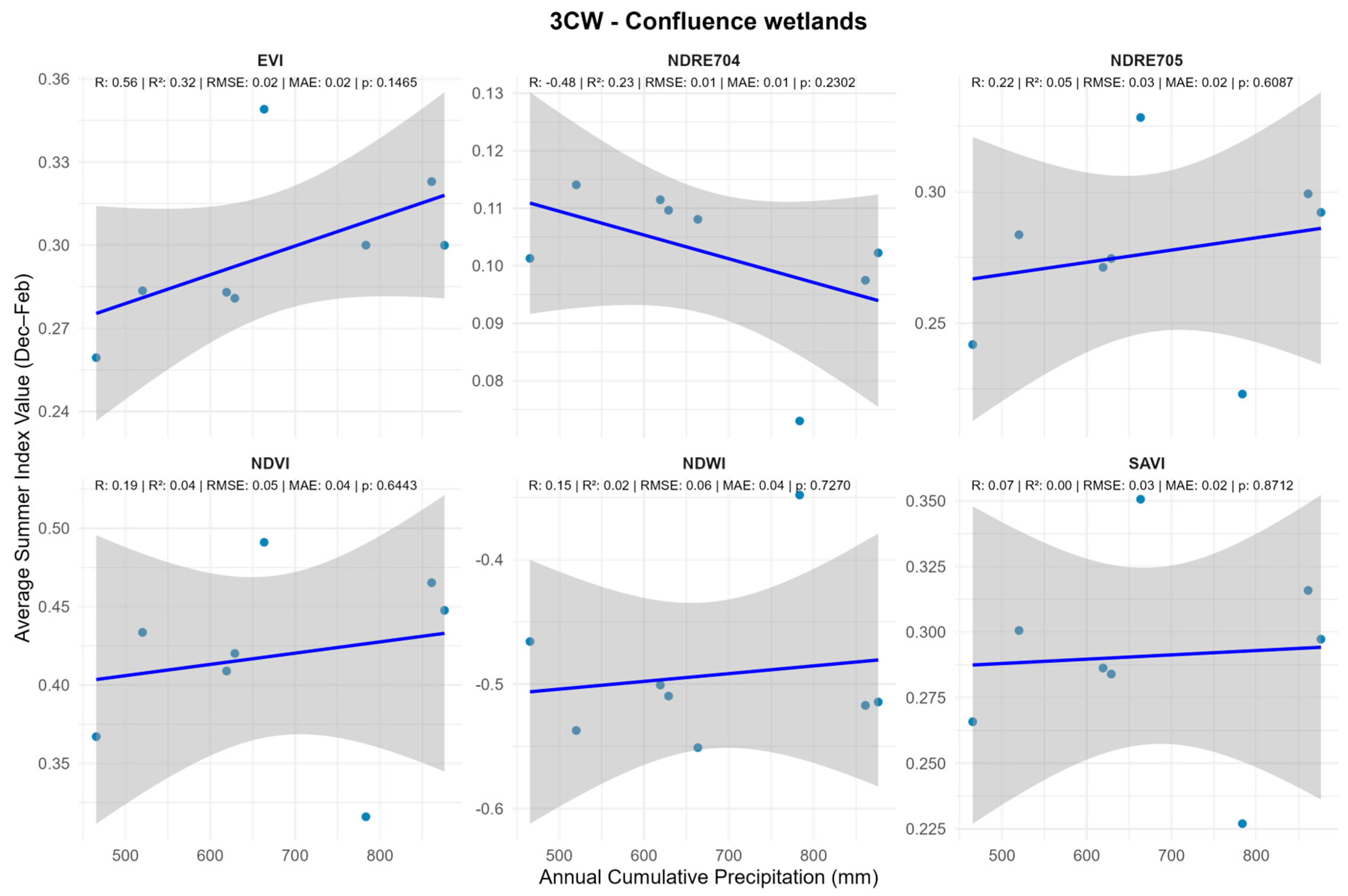
- Confluence wetland (3CW): In the confluence wetland, the correlations between the previous year’s cumulative annual precipitation and the spectral indices yielded the following values:
Indices with positive correlation
- EVI: R = 0.56; R² = 0.32; p = 0.15
- NDRE705: R = 0.22; R² = 0.05; p = 0.61
- NDVI: R = 0.19; R² = 0.04; p = 0.64
- NDWI: R = 0.06; R² = 0.02; p = 0.73
- SAVI: R = 0.07; R² = 0.00; p = 0.87
Indices with negative correlation
- NDRE704: R = –0.48; R² = 0.23; p = 0.23
In terms of statistical significance, none of the indices evaluated presented statistically significant values (p < 0.05). The values of the goodness-of-fit metrics presented the following error ranges:
- RMSE: 0.01–0.06
- MAE: 0.01–0.04
Figure 10.
Linear correlation between previous-year annual precipitation and summer vegetation indices for the confluence wetland (3CW).
Figure 10.
Linear correlation between previous-year annual precipitation and summer vegetation indices for the confluence wetland (3CW).
3.3. Multitemporal Color Composites
Multitemporal analysis using color mosaics was performed only for spectral indices that showed the best statistical performance in each wetland, as measured by linear correlation (R), coefficient of determination (R²), and significance (p-value). The maximum and minimum values were extracted directly from the monthly series for each available date (2018–2025), enabling quantitative characterization of interannual variation in vegetation vigor and the dominant spectral signal at each site.
- Header wetland (1HW)
The indices selected for this wetland were NDVI, NDRE705, and NDWI, which showed the highest and most significant correlations with the previous year’s precipitation.
- ➔
- NDVI
The NDVI in the headwater wetland ranged from 0.25 to 0.85. The period between 2018 and 2021 recorded the highest values, during which they mainly ranged from 0.60 to 0.80, indicating a consistent presence of dense vegetation. Starting in 2022, the index declined to intermediate levels (0.40–0.65) and, finally, in 2024–2025, the lowest greenness intensity was observed, with reduced ranges between 0.30 and 0.55, especially in the central and lower areas of the wetland (Figure 11).
- ➔
- NDRE705
The NDRE705 recorded values that fluctuated between 0.09 and 0.18 throughout the evaluation period. The period between 2019 and 2021 showed the highest values, when the index ranged from 0.15 to 0.18, suggesting a higher concentration of chlorophyll and greater photosynthetic activity. Since 2022, the index has decreased to intermediate values between 0.10 and 0.14, maintaining a more stable but lower signal (Figure 12).
- ➔
- NDWI
The NDWI ranged from –0.30 to 0.12, reflecting significant variations in surface moisture. The highest values for the period (between 0.00 and 0.12) were recorded between 2019 and 2021, while negative values between –0.30 and –0.05 predominated from 2022 onwards, consistent with drier conditions in the central and lower sectors of the wetland (Figure 13).
- Lateral Wetland (2LW)
The indices selected for this wetland were NDVI, NDRE705, and EVI, which showed the highest and most significant correlations with the previous year’s precipitation.
- ➔
- NDVI
The NDVI in the lateral wetland ranged from 0.20 to 0.78. The analysis observed the highest values between 2018 and 2021, with values predominantly between 0.60 and 0.75, especially along the central axis of the wetland. From 2022 onward, the NDVI decreased to intermediate values (0.40–0.60), and in 2024–2025, the lowest values were recorded, ranging from 0.30 to 0.50, indicating a reduction in vegetation vigor (Figure 14).
- ➔
- NDRE705
The NDRE705 ranged from 0.08 to 0.17. The years 2020–2021 had the highest values (0.14-0.17), associated with higher chlorophyll content. From 2022 onwards, the ranges decreased to intervals of 0.09–0.13, with greater spatial variability and lower intensity in the southern and central areas (Figure 15).
- ➔
- EVI
The EVI ranged from 0.15 to 0.55. Between 2018 and 2021, the highest values were recorded, with a typical range of 0.40 to 0.55. Subsequently, in 2022–2025, the index shifted toward lower values, ranging from 0.25 to 0.40, suggesting a downward trend in summer vegetation vigor (Figure 16).
- Confluence wetland (3CW)
The indices selected for this wetland were EVI and NDRE704, which showed the highest and most significant correlations with the previous year’s precipitation.
- ➔
- EVI
The EVI in the confluence wetland ranged from 0.10 to 0.48. We observed the highest values between 2018 and 2021 (0.32-0.48), reflecting more active vegetation in the central sectors. Since 2022, the index has shown a progressive decline, ranging from 0.20 to 0.35, while in 2024–2025, the lowest values on record (0.10-0.25) were observed (Figure 17).
- ➔
- NDRE704
The NDRE704 ranged between 0.06 and 0.13. The highest values were recorded between 2020 and 2021, with values ranging from 0.11 to 0.13 indicating higher chlorophyll levels. Since 2022, values have fallen to 0.07-0.10, maintaining a reduced, relatively homogeneous signal across most of the wetland (Figure 18).
4. Discussion
The high-Andean wetlands of the SNLN are located in a hydroclimatic context characterized by substantial interannual variability in precipitation and the megadrought affecting central Chile since 2010 [8,9]. Precipitation is the primary hydrological determinant of these ecosystems, regulating the availability of surface and groundwater, soil saturation, and summer plant productivity [6,7,18,19,20]. In this scenario, evaluating vegetation responses using spectral indicators derived from Sentinel-2 allows us to characterize structural and functional changes associated with the water regime.
4.1. State of Wetlands and Expected Response to the Climate Context
The results reflect contrasting behaviors among the three functional types of wetlands analyzed. The headwater wetland showed the greatest sensitivity to interannual climate variability, with sustained increases in NDVI, EVI, and SAVI between 2018 and 2025, along with a progressive decrease in NDWI. This pattern, consistent with previous studies in high Andean wetlands dependent on snowmelt recharge [6,19], suggests that years with higher antecedent precipitation favored greater vegetation vigor, but also higher summer water consumption.
The lateral wetland showed more pronounced fluctuations and less consistent trends, as expected in systems with intermediate hydrological connectivity, gentle slopes, and greater soil exposure, where local topographic factors modulate the spectral response [7,21,22]. In contrast, the confluence wetland showed overall stability in the indices evaluated, consistent with ecosystems that receive contributions from lateral and subsurface flow that buffer short-term climate variability [21,25].
4.2. Contributions from the Combined Use of Spectral Indices and Climate Data
The integrated analysis of multispectral indices and accumulated precipitation (lag-1) allowed us to identify ecohydrological relationships consistent with the expected dynamics for mountain wetlands. In the headwater wetland, NDVI and NDRE705 showed positive, significant correlations with previous precipitation (R = 0.79; p < 0.05), indicating a direct dependence on the water regime of the last cycle. This type of delayed response has been widely described in mountain ecosystems, where vegetation depends on winter storage rather than immediate precipitation [6,7,18].
In the lateral wetland, correlations were moderate and insignificant, evidencing the influence of local factors in addition to precipitation. The confluence wetland showed very low correlations, suggesting more stable functioning and less dependence on interannual rainfall variability [25].
Multitemporal mosaics supported these results, showing maximum vegetation vigor between 2018 and 2021, followed by a progressive decline toward 2024–2025, consistent with the transition from wet years to a drier period, as documented in recent studies in Andean wetlands of the Altiplano and the Cordillera Blanca [19,22,25].
4.3. Strengths and Limitations of the Applied Approach
The combined use of Sentinel-2 images, ERA5-Land data, and UAV flights exclusively dedicated to the precise delimitation of wetlands provided a solid basis for analyzing the ecohydrological dynamics of the SNLN. The multiscale approach enabled capturing both subtle changes in vegetation (NDRE, NDVI) and variations in surface moisture (NDWI) with a level of detail appropriate for small-scale ecosystems with high spatial heterogeneity [12,13,15,26]. However, the study has limitations:
- The spectral response may be saturated in areas of high biomass (NDVI, EVI) [11]
- NDWI is sensitive to spectral mixing between vegetation, water, and shade [15,16]
- Linear models may underestimate nonlinear behaviors or ecohydrological thresholds [26]
- The time series (2018–2025) coincides with a period of extreme weather, which may influence the interpretation of trends.
These challenges are consistent with recent recommendations promoting the integration of hyperspectral and thermal sensors and machine learning-based models to improve the characterization of complex wetlands [26,27].
4.5. Relevance for the Monitoring and Future Management of High Andean Wetlands
The results reinforce the fact that wetlands do not respond uniformly to climate variability. The headwater wetland emerges as an indicator site sensitive to regional hydrological conditions. In contrast, lateral and confluence wetlands require integrating geomorphological metrics, local hydrological information, and spatial modeling to understand their functioning fully [21,25].
The combination of satellite imagery and UAV delimitation provides a robust, replicable tool for adaptive monitoring of high-Andean wetlands under scenarios of prolonged drought and increased temperatures projected by the IPCC [1].
5. Conclusions
This study integrated Sentinel-2 imagery, ERA5-Land climate data, and UAV delineations to evaluate vegetation dynamics in three high-Andean wetlands within the Los Nogales Nature Sanctuary between 2018 and 2025. The results showed that the previous year’s cumulative annual precipitation is a determining factor in the summer spectral response, especially in the headwater wetland (1HW), where indices such as NDVI and NDRE705 showed significant correlations (R = 0.79; p < 0.05). This behavior confirms the dependence of these ecosystems on the processes of snow accumulation and deep infiltration described in high Andean wetlands and semi-arid areas [6,7,18].
Multitemporal mosaics revealed a period of greater vegetative vigor between 2018 and 2021, followed by a progressive decline toward 2024–2025, coinciding with rainfall deficits during the megadrought in central Chile [8,9] and with the global temperature increase observed [1,2]. The wetlands showed different responses: the headwaters were most sensitive to water variability, the lateral wetland exhibited intermediate fluctuations, and the confluence wetland showed relative stability, consistent with systems where surface and groundwater flows converge [19,21,25].
Methodologically, the combination of vegetation indices (NDVI, EVI, SAVI), red-edge bands (NDRE704–705), and NDWI allowed for a comprehensive characterization of the structure, vigor, and moisture content of the vegetation cover, confirming the value of multiscale approaches based on remote sensing for monitoring mountain wetlands [12,13,15,26]. High-resolution delimitation using UAVs improved the spatial accuracy of satellite analyses, although we did not use it as spectral input.
Taken together, the results show that high-Andean wetlands respond differently to climate variability, and that integrating multi-temporal remote sensing series is an effective tool for their monitoring and adaptive management. This approach provides a solid basis for strengthening the conservation of these vulnerable ecosystems and can guide applications to other high Andean systems with similar characteristics.
Author Contributions
Conceptualization, F.L.-B., L.D.-G. and W.P.-M.; methodology, J.G.-L. and L.D.-G.; software, J.G.-L. and B.C.-C.; validation, J.G.-L. and B.C.-C.; formal analysis, J.G.-L.; investigation, J.G.-L. and F.L.-B.; resources, W.P.-M.; data curation, J.G.-L. and B.C.-C.; writing—original draft preparation, F.L.-B.; writing—review and editing, L.D.-G., W.P.-M. and J.G.-L.; visualization, J.G.-L. and B.C.-C.; supervision, L.D.-G. and W.P.-M.; project administration, L.D.-G.; funding acquisition, W.P.-M. and L.D.-G. All authors have read and agreed to the published version of the manuscript.
Funding
This research was funded by Anglo American Chile, contract number 5.23.0022.1 “Servicio de Estudios de Conservación de Humedales Altoandinos Hijuela C en Santuario de la Naturaleza Los Nogales”.
Institutional Review Board Statement
Not applicable.
Informed Consent Statement
Not applicable.
Data Availability Statement
Restrictions apply to the availability of these data. The datasets were obtained from Anglo American Chile under a service contract and are therefore not publicly available. Data may be requested from the corresponding author with the permission of Anglo American Chile.
Conflicts of Interest
The authors declare no conflicts of interest.
References
- IPCC. Climate Change 2023: Synthesis Report. Contribution of Working Groups I, II and III to the Sixth Assessment Report of the Intergovernmental Panel on Climate Change; Core Writing Team, Lee, H., Romero, J., Eds.; IPCC: Geneva, Switzerland, 2023; pp. 1–34. [CrossRef]
- World Meteorological Organization (WMO). The World Meteorological Organization confirms that 2024 was the warmest year on record, exceeding pre-industrial levels by approximately 1.55 °C. Available online: https://wmo.int/es/news/media-centre/la-organizacion-meteorologica-mundial-confirma-que-2024-fue-el-ano-mas-calido-jamas-registrado-al (accessed on 18 February 2025).
- Ministerio del Medio Ambiente. Humedales y Turberas en Chile: Relevancia, Amenazas y Desafíos para su Conservación; Centro de Estudios de Medio Ambiente, Universidad Austral de Chile: Valdivia, Chile, 2017. Available online: https://obtienearchivo.bcn.cl/obtienearchivo?id=repositorio/10221/24257/2/Humedales_y_turberas_en_Chile_CMA_2017_FINAL.pdf (accessed on 15 January 2024).
- Alvis-Ccoropuna, T.; Villasante-Benavides, J.F.; Pauca-Tanco, G.A.; Quispe-Turpo, J.P.; Luque-Fernández, C.R. Cálculo y valoración del almacenamiento de carbono del humedal altoandino de Chalhuanca, Arequipa (Perú). Rev. Investig. Altoandinas 2021, 23, 139–148. [CrossRef]
- Sciolla, D.; Bustos, E. Monitoreo de los Humedales Altoandinos en la Cuenca del Río Maipo: Estudio Base sobre la Importancia de la Conservación de la Infraestructura Verde para la Seguridad Hídrica; Santiago, Chile, 2023.
- de la Fuente, A.; Meruane, C.; Suárez, F. Long-term spatiotemporal variability in high Andean wetlands in northern Chile. Sci. Total Environ. 2021, 754, 143830. [CrossRef]
- Duhalde, D.; Cortés, J.; Arumí, J.-L.; Boll, J.; Oyarzún, R. Exploring the behavior of the high-Andean wetlands in the semi-arid zone of Chile: The influence of precipitation and temperature variability on vegetation cover and water quality. Water 2024, 16, 3682. [CrossRef]
- Garreaud, R.D.; Alvarez-Garreton, C.; Barichivich, J.; Boisier, J.P.; Christie, D.; Galleguillos, M.; LeQuesne, C.; McPhee, J.; Zambrano-Bigiarini, M. The 2010–2015 megadrought in central Chile: Impacts on regional hydroclimate and vegetation. Hydrol. Earth Syst. Sci. 2017, 21, 6307–6327. [CrossRef]
- Garreaud, R.D.; Boisier, J.P.; Rondanelli, R.; Montecinos, A.; Sepúlveda, H.H.; Veloso-Aguila, D. The central Chile megadrought (2010–2018): A climate dynamics perspective. Int. J. Climatol. 2019, 40, 421–439. [CrossRef]
- Rouse, J.W.; Haas, R.H.; Schell, J.A.; Deering, D.W. Monitoring vegetation systems in the Great Plains with ERTS. In Proceedings of the Third Earth Resources Technology Satellite-1 Symposium; NASA: Washington, DC, USA, 1973; pp. 309–317.
- Huete, A. R., Didan, K., Miura, T., Rodriguez, E. P., Gao, X., & Ferreira, L. G. (2002). Overview of the radiometric and biophysical performance of the MODIS vegetation indices. Remote Sensing of Environment, 83(1–2), 195–213. [CrossRef]
- Barnes, E. M., Clarke, T. R., Richards, S. E., Colaizzi, P. D., Haberland, J., Kostrzewski, M., … Lascano, R. J. (2000, July). Coincident detection of crop water stress, nitrogen status and canopy density using ground-based multispectral data. Proceedings of the Fifth International Conference on Precision Agriculture (pp. 1–15). https://www.tucson.ars.ag.gov/unit/publications/PDFfiles/1356.pdf.
- Clevers, J. G. P. W., & Gitelson, A. A. (2013). Remote estimation of crop and grass chlorophyll and nitrogen content using red-edge bands on Sentinel-2 and -3. International Journal of Applied Earth Observation and Geoinformation, 23, 344–351. [CrossRef]
- Rouse, J. W., Jr., Haas, R. H., Schell, J. A., & Deering, D. W. (1974). Monitoring vegetation systems in the Great Plains with ERTS. En S. C. Freden, E. P. Mercanti, & M. A. Becker (Eds.), Third Earth Resources Technology Satellite-1 Symposium (NASA SP-351), Vol. 1: Technical Presentations (pp. 309–317). NASA. https://ntrs.nasa.gov/citations/19740022614.
- Gao, B.-C. (1996). NDWI—A normalized difference water index for remote sensing of vegetation liquid water from space. Remote Sensing of Environment, 58(3), 257–266.
- McFeeters, S. K. (1996). The use of the normalized difference water index (NDWI) in the delineation of open water features. International Journal of Remote Sensing, 17(7), 1425–1432. [CrossRef]
- Huete, A. R. (1988). A soil-adjusted vegetation index (SAVI). Remote Sensing of Environment, 25(3), 295–309. [CrossRef]
- He, Y. The effect of precipitation on vegetation cover over three landscape units in a protected semi-arid grassland: Temporal dynamics and suitable climatic index. J. Arid Environ. 2014, 109, 74–82. [CrossRef]
- Chimner, R.A.; Bourgeau-Chavez, L.; Grelik, S.; Hribljan, J.A.; Clarke, A.M.P.; Polk, M.H.; Lilleskov, E.A.; Fuentealba, B. Mapping mountain peatlands and wet meadows using multi-date, multi-sensor remote sensing in the Cordillera Blanca, Peru. Wetlands 2019, 39, 1057–1067. [CrossRef]
- Ali, S.; Basit, A.; Umair, M.; Makanda, T.A.; Khan, F.U.; Shi, S.; Ni, J. Spatio-temporal variations in trends of vegetation and drought changes in relation to climate variability from 1982 to 2019 based on remote sensing data from East Asia. J. Integr. Agric. 2023, 22, 3193–3208. [CrossRef]
- Otto, M., Scherer, D., & Richters, J. (2011). Hydrological differentiation and spatial distribution of high altitude wetlands in a semi-arid Andean region derived from satellite data. Hydrology and Earth System Sciences, 15(5), 1713–1727. [CrossRef]
- Castillo, D., Russell, A., Caquilpan, V., & Elgueta, S. (2020). Identification of affected high-altitude wetlands in north Chile using large Landsat time series. ISPRS Archives, XLII-3/W12, 13–18. [CrossRef]
- Duhalde, D., Cortés, J., Arumí, J.-L., Boll, J., & Oyarzún, R. (2024). Exploring the behavior of high-Andean wetlands in the semi-arid zone of Chile: The influence of precipitation and temperature variability on vegetation cover and water quality. Water, 16(24), 3682. [CrossRef]
- Paquis, P., Hengst, M. B., Florez, J. Z., Tapia, J., Molina, V., Pérez, V., & Pardo-Esté, C. (2023). Short-term characterisation of climatic-environmental variables and microbial community diversity in a high-altitude Andean wetland (Salar de Huasco, Chile). Science of The Total Environment, 859(Pt 2), 160291. [CrossRef]
- Huaraca, L., Lopera, A., Villacreses, A., & Aguilar, E. (2025). Multitemporal monitoring of Ecuadorian Andean high-altitude wetlands. Water, 17(11), 1637. [CrossRef]
- Jafarzadeh, H.; Mahdianpari, M.; Gill, E.W.; Brisco, B.; Mohammadimanesh, F. Remote sensing and machine learning tools to support wetland monitoring: A meta-analysis of three decades of research. Remote Sens. 2022, 14, 6104. [CrossRef]
- Zhao, A.; Cheng, X.; Cao, R.; Huang, L.; Hou, Z. Continuous monitoring of forests in wetland ecosystems with remote sensing and probability sampling. Remote Sens. 2024, 16, 3508. [CrossRef]
- Gitelson, A. A., Kaufman, Y. J., Stark, R., & Rundquist, D. (2002). Novel algorithms for remote estimation of vegetation fraction. Remote Sensing of Environment, 80(1), 76–87. [CrossRef]
- Meyer, G. E., & Neto, J. C. (2008). Verification of color vegetation indices for automated crop imaging applications. Computers and Electronics in Agriculture, 63(2), 282–293. [CrossRef]
- Hunt, E. R., Daughtry, C. S. T., Eitel, J. U. H., & Long, D. S. (2011). Remote sensing leaf chlorophyll content using a visible band index. Agronomy Journal, 103(4), 1090–1099. [CrossRef]
- Muñoz-Sabater, J.; Dutra, E.; Agustí-Panareda, A.; Albergel, C.; Arduini, G.; Balsamo, G.; et al. ERA5-Land: A State-of-the-Art Global Reanalysis Dataset for Land Applications. Earth Syst. Sci. Data 2021, 13(9), 4349–4383. [CrossRef]
- Gorelick, N.; Hancher, M.; Dixon, M.; Ilyushchenko, S.; Thau, D.; Moore, R. Google Earth Engine: Planetary-Scale Geospatial Analysis for Everyone. Remote Sens. Environ. 2017, 202, 18–27. [CrossRef]
- European Space Agency (ESA). Copernicus Browser: Access to Sentinel Satellite Data. ESA Copernicus Open Access Hub, 2024. Available online: https://browser.dataspace.copernicus.eu (accessed on 26 September 2025).
- López, M.; García, L.; Rivas, R.; Aguilar, C. Evaluation of NDVI Thresholds for Vegetation Condition Monitoring in Semi-Arid Regions. J. Arid Environ. 2015, 120, 23–32. [CrossRef]
- Esri. Site Scan for ArcGIS: Drone Mapping & Analytics Software. Esri, Redlands, CA, USA, 2024. Available online: https://www.esri.com/en-us/arcgis/products/arcgis-reality/products/site-scan-for-arcgis (accessed on 26 September 2025).
- R Core Team. R: A Language and Environment for Statistical Computing; R Foundation for Statistical Computing: Vienna, Austria, 2023. Available online: https://www.R-project.org/ (accessed on 26 September 2025).
- RStudio Team. RStudio: Integrated Development Environment for R; RStudio, PBC: Boston, MA, USA, 2023. Available online: https://posit.co/products/open-source/rstudio/ (accessed on 26 September 2025).
- Pearson, K. (1895). Note on Regression and Inheritance in the Case of Two Parents. Proceedings of the Royal Society of London, 58, 240–242. [CrossRef]
- Willmott, C. J., & Matsuura, K. (2005). Advantages of the Mean Absolute Error (MAE) over the Root Mean Square Error (RMSE) in Assessing Average Model Performance. Climate Research, 30(1), 79–82. [CrossRef]
- Draper, N. R., & Smith, H. (1998). Applied Regression Analysis (3rd ed.). Wiley Series in Probability and Statistics. John Wiley & Sons, Inc. [CrossRef]
- Steel, R.G.D., Torrie, J.H. and Dicky, D.A. (1997) Principles and Procedures of Statistics, A Biometrical Approach. 3rd Edition, McGraw Hill, Inc. Book Co., New York, 352-358.
Figure 1.
Study area.
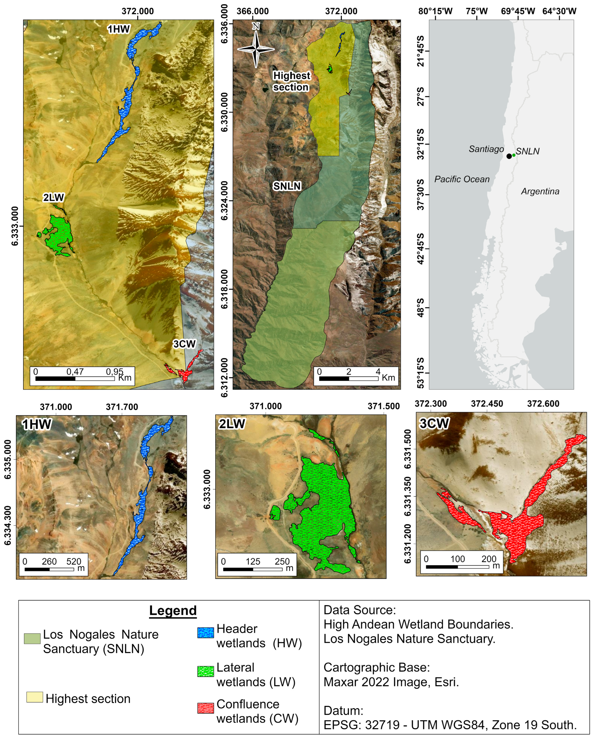
Figure 2.
Methodological workflow for the acquisition, processing, and analysis of remote sensing data used to evaluate vegetation–climate relationships in high-Andean wetlands (2018–2025).
Figure 2.
Methodological workflow for the acquisition, processing, and analysis of remote sensing data used to evaluate vegetation–climate relationships in high-Andean wetlands (2018–2025).
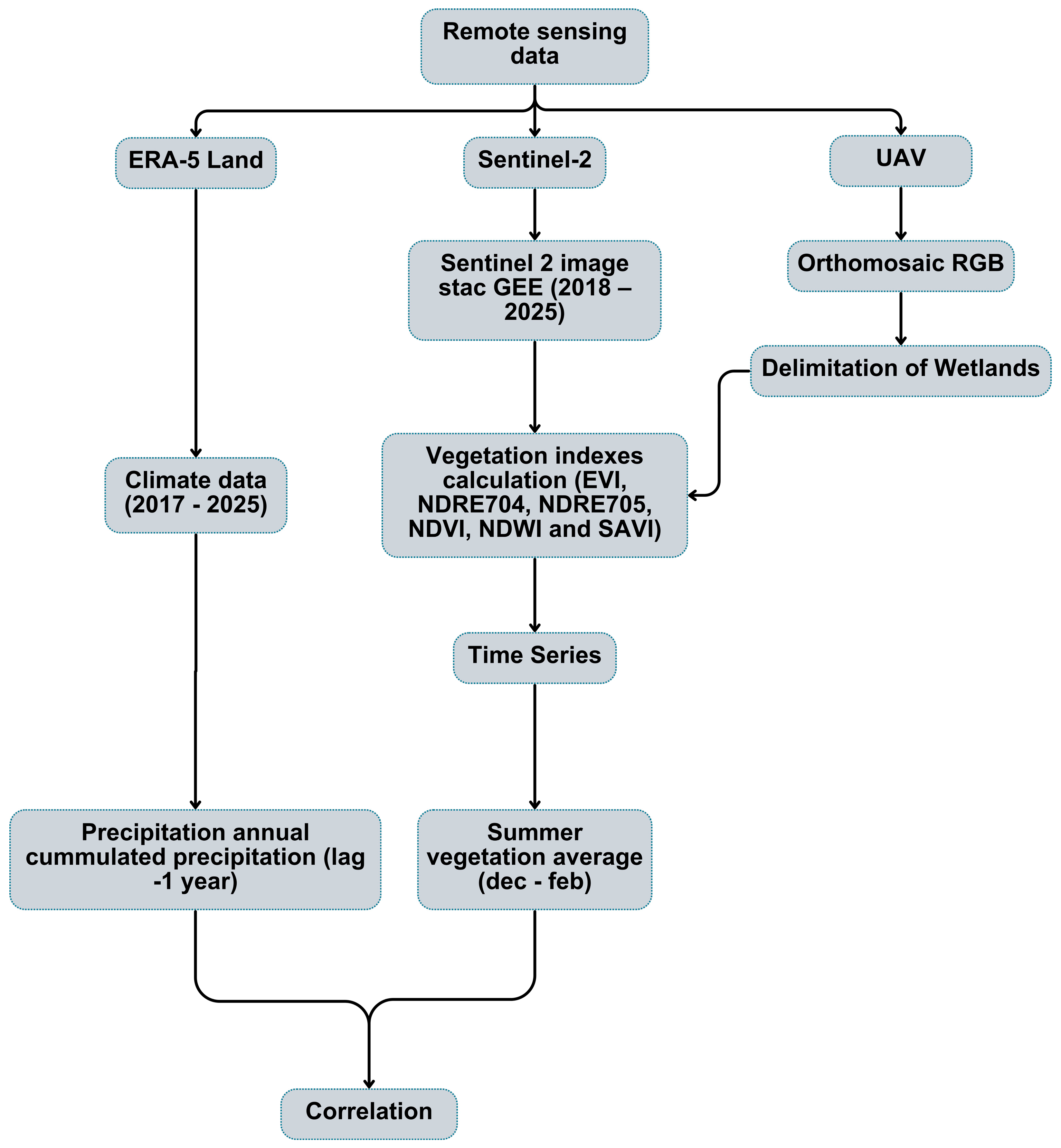
Figure 3.
Annual cumulative precipitation (mm) for the period 2017–2025 derived from ERA5-Land.
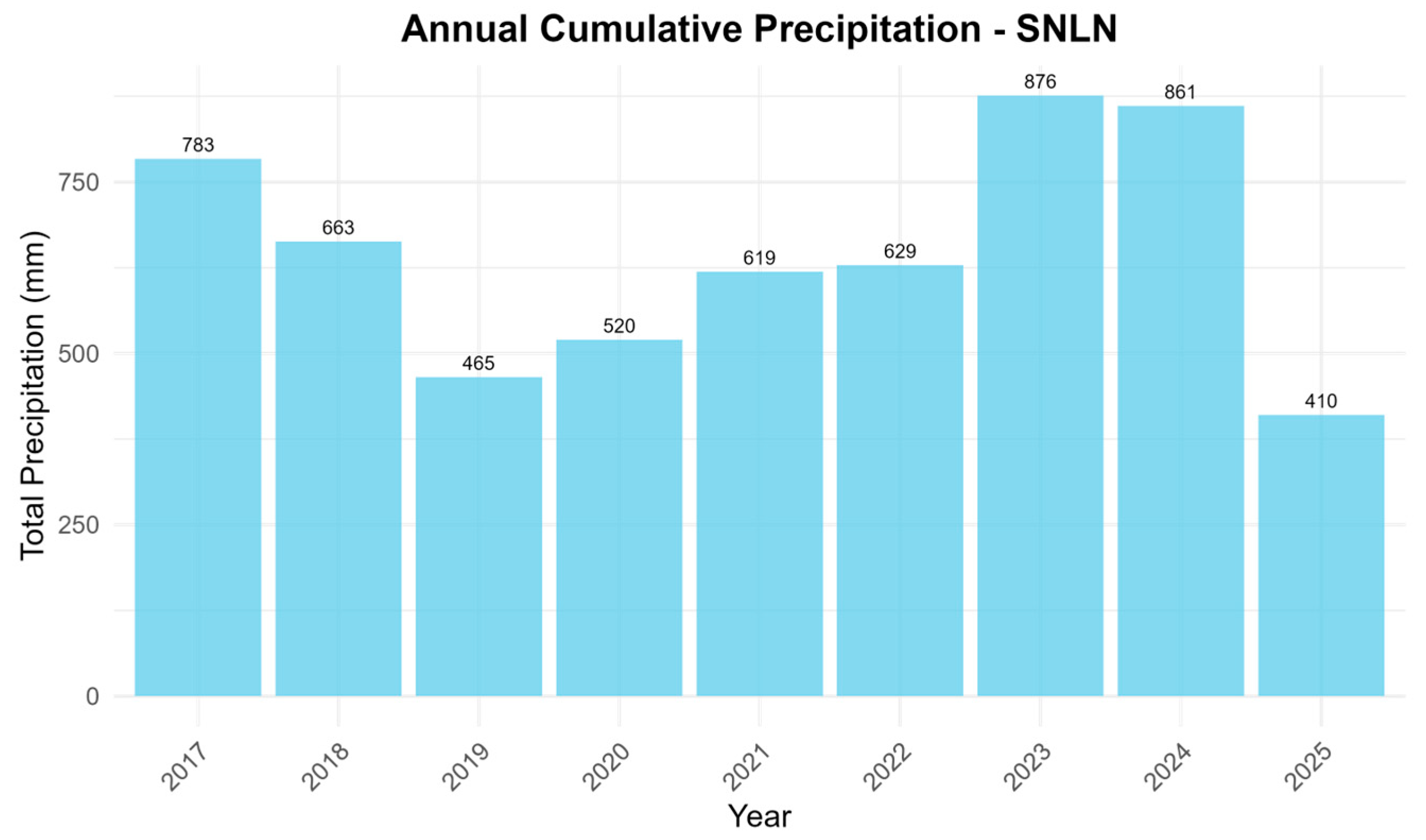
Figure 4.
Monthly precipitation (mm) and linear trend derived from ERA5-Land for the period 2017–2025.
Figure 4.
Monthly precipitation (mm) and linear trend derived from ERA5-Land for the period 2017–2025.
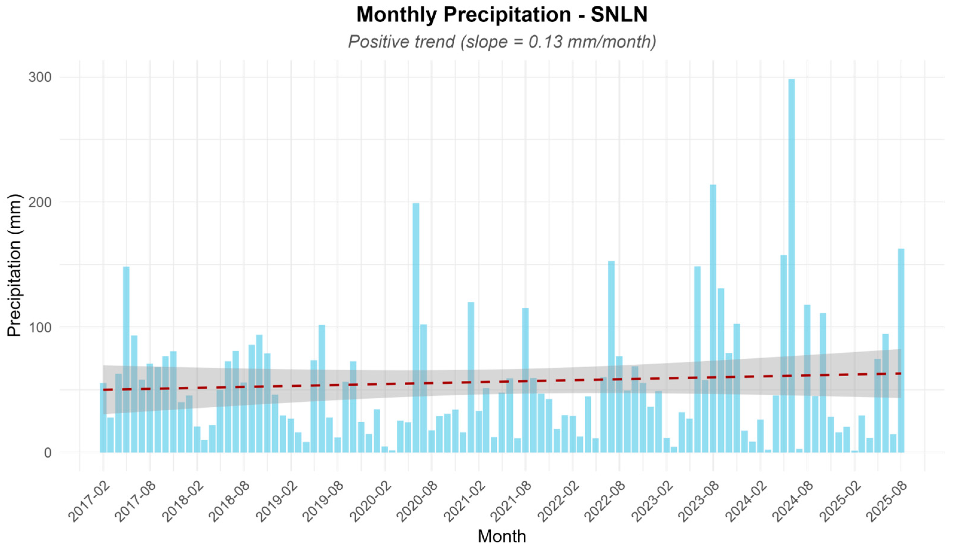
Figure 5.
Temporal trends of vegetation and water indices in headwater wetlands (2018–2025).
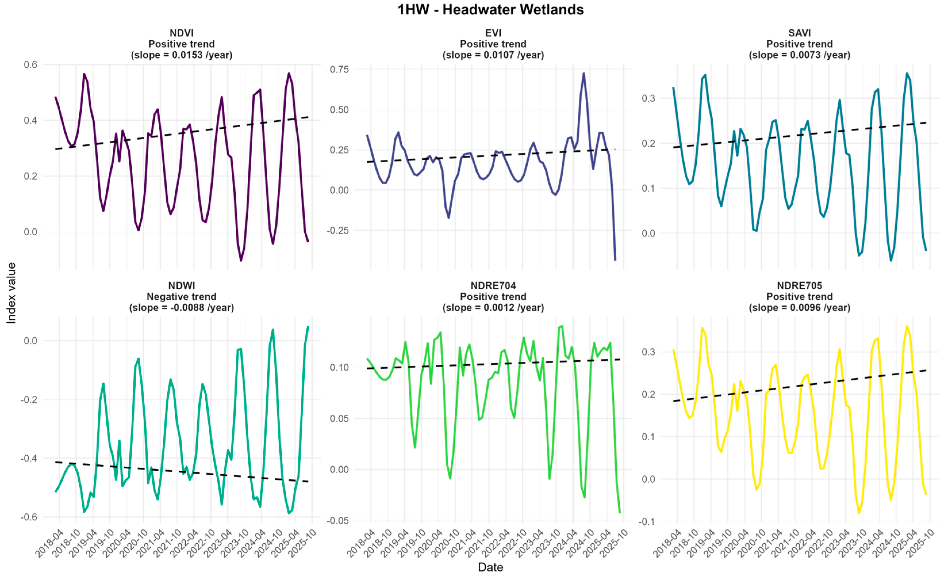
Figure 6.
Temporal trends of vegetation and water indices in lateral wetlands (2018–2025).
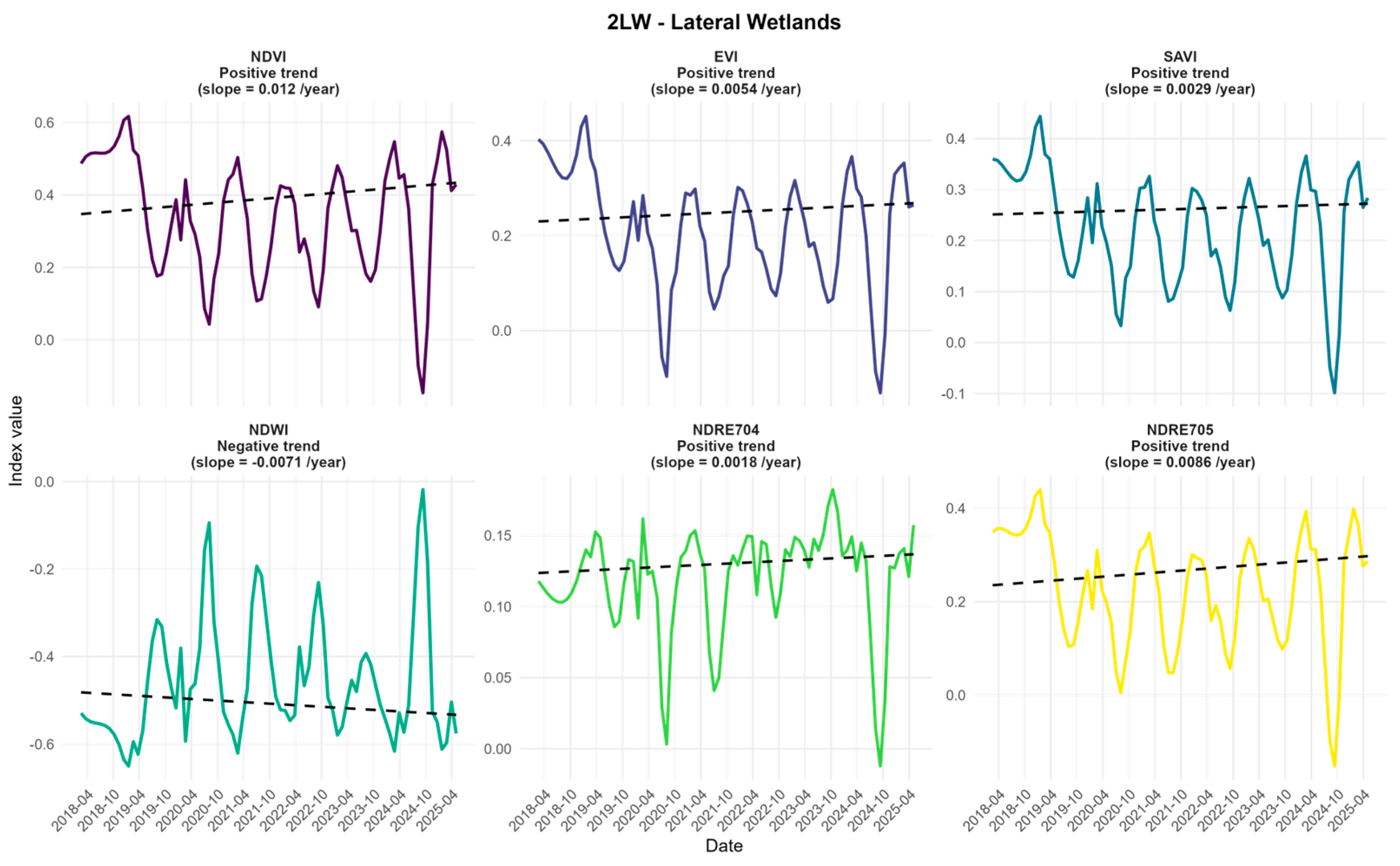
Figure 7.
Temporal trends of vegetation and water indices in confluence wetlands (2018–2025).
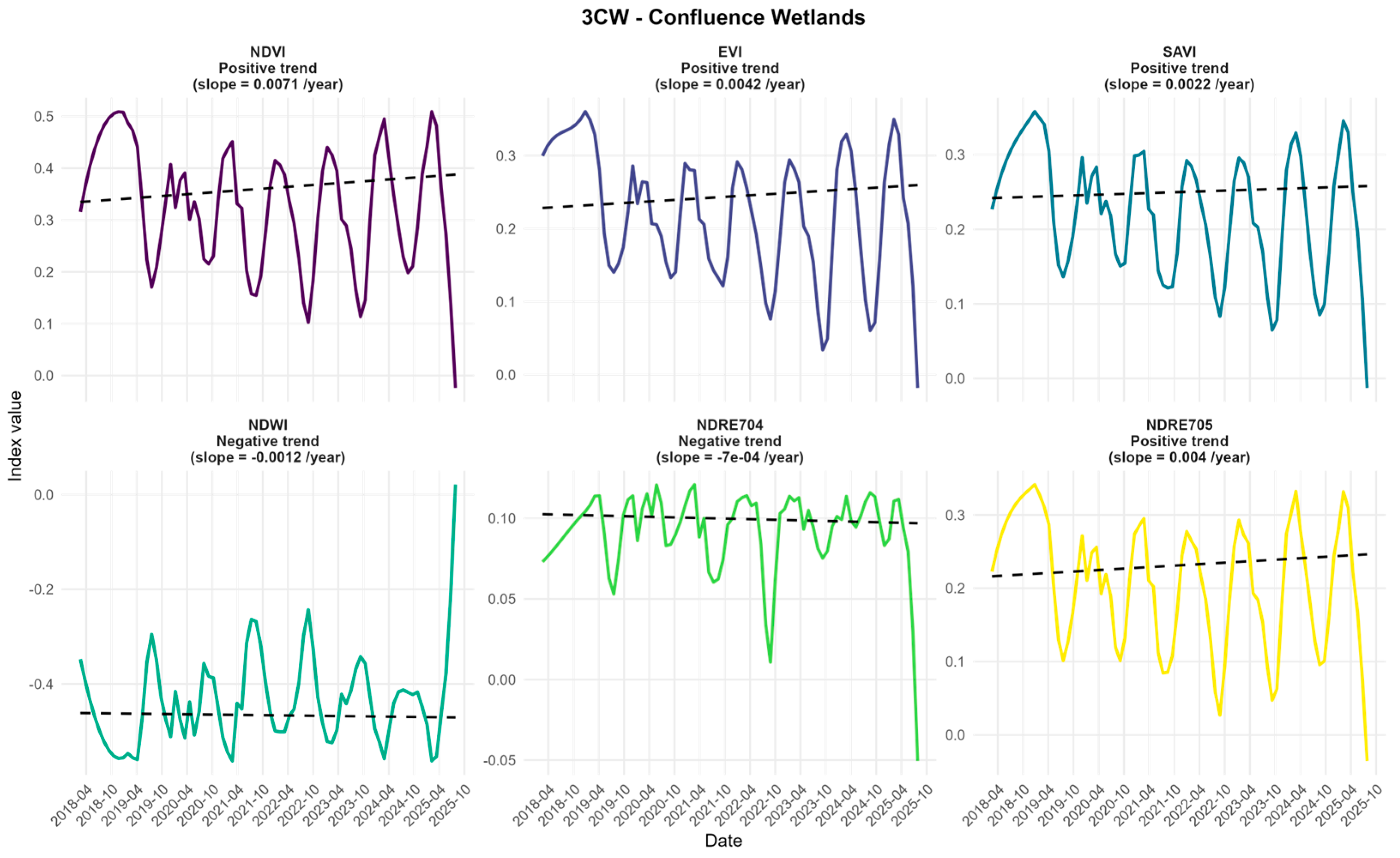
Figure 8.
Linear correlation between previous-year annual precipitation and summer vegetation indices for the headwater wetland (1HW).
Figure 8.
Linear correlation between previous-year annual precipitation and summer vegetation indices for the headwater wetland (1HW).
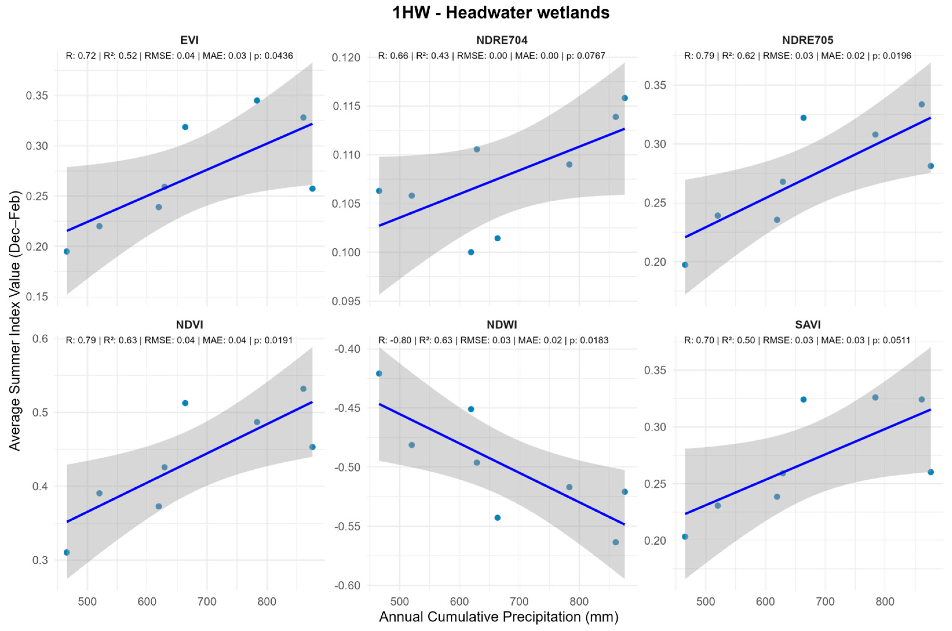
Figure 9.
Linear correlation between previous-year annual precipitation and summer vegetation indices for the lateral wetland (2LW).
Figure 9.
Linear correlation between previous-year annual precipitation and summer vegetation indices for the lateral wetland (2LW).
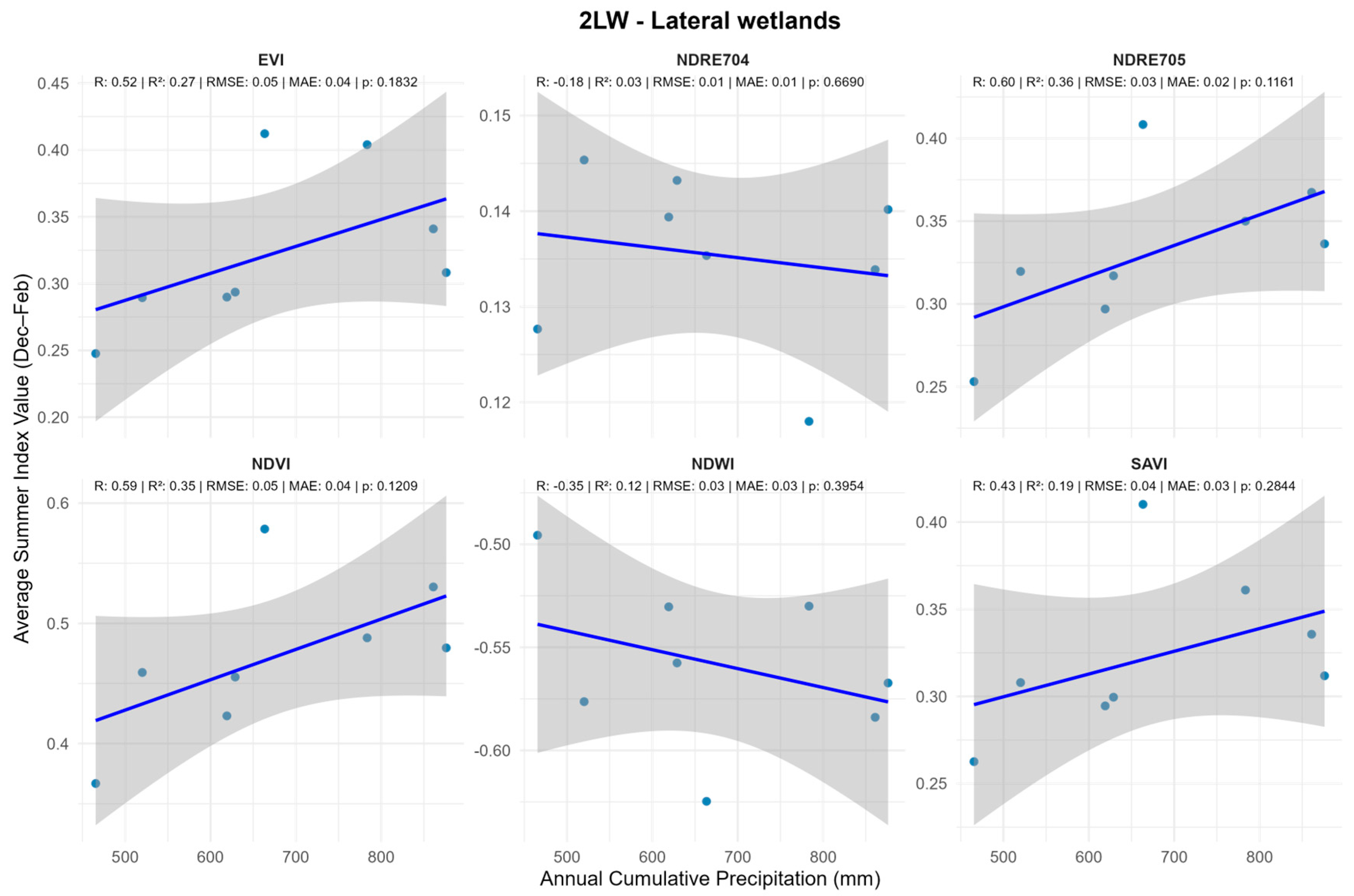
Figure 11.
Multitemporal NDVI color composite for the Headwater wetland (2018–2025) derived from Sentinel-2 imagery during the summer season.
Figure 11.
Multitemporal NDVI color composite for the Headwater wetland (2018–2025) derived from Sentinel-2 imagery during the summer season.
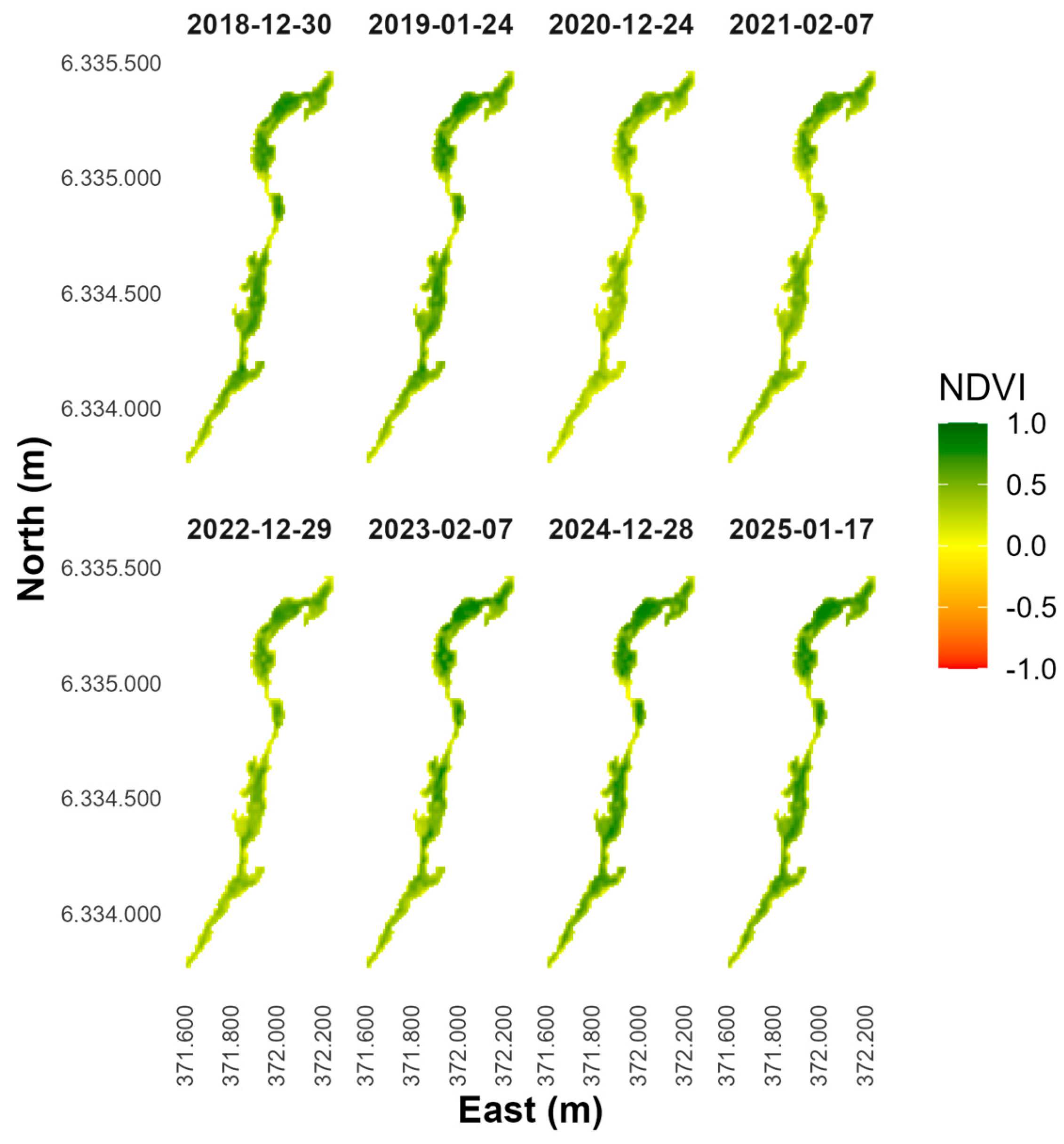
Figure 12.
Multitemporal NDRE705 color composite for the Headwater wetland (2018–2025) showing subtle changes in photosynthetic activity and vegetation density.
Figure 12.
Multitemporal NDRE705 color composite for the Headwater wetland (2018–2025) showing subtle changes in photosynthetic activity and vegetation density.
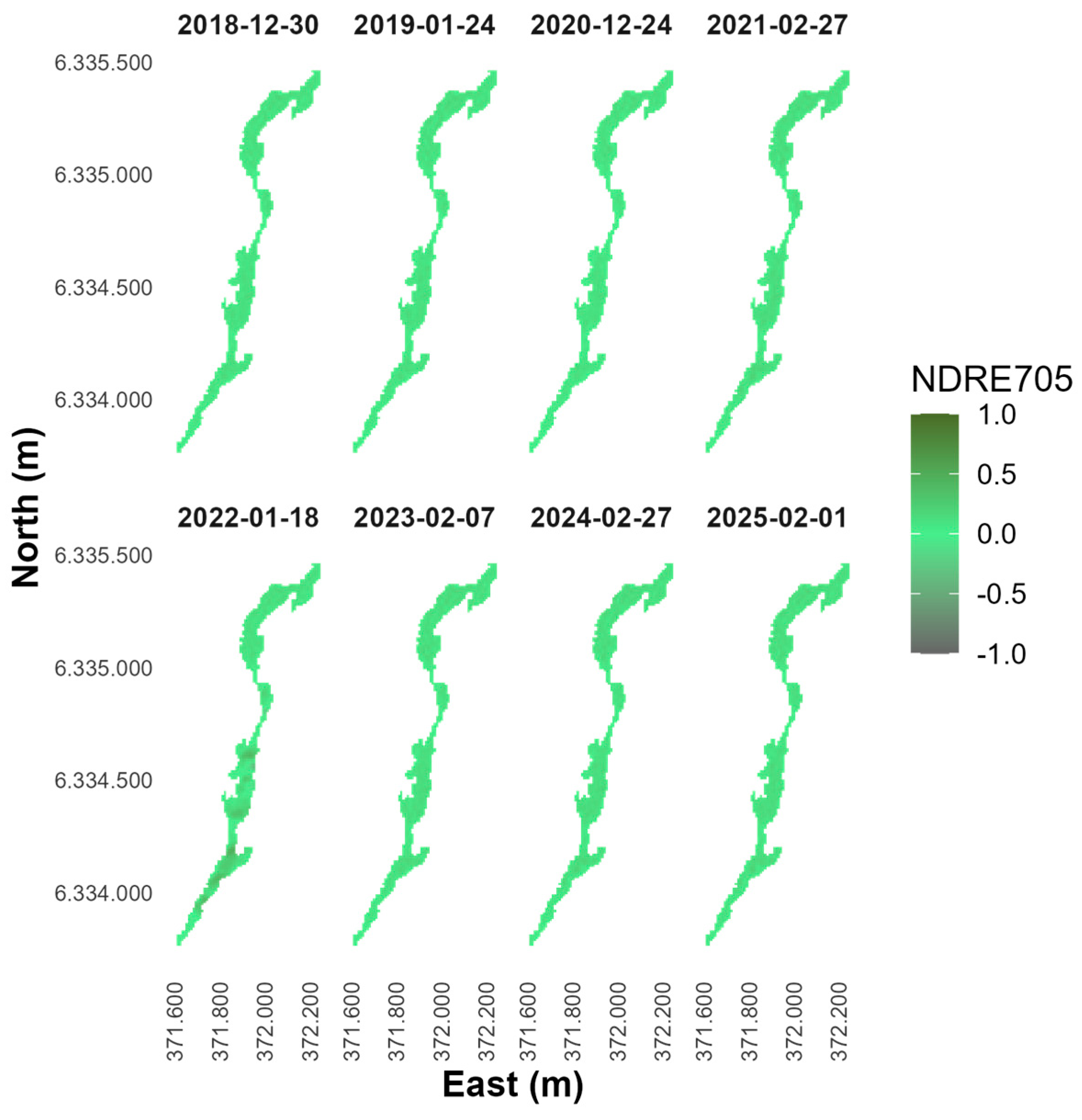
Figure 13.
Multitemporal NDWI color composite for the Headwater wetland (2018–2025) indicating temporal variations in surface water content.
Figure 13.
Multitemporal NDWI color composite for the Headwater wetland (2018–2025) indicating temporal variations in surface water content.
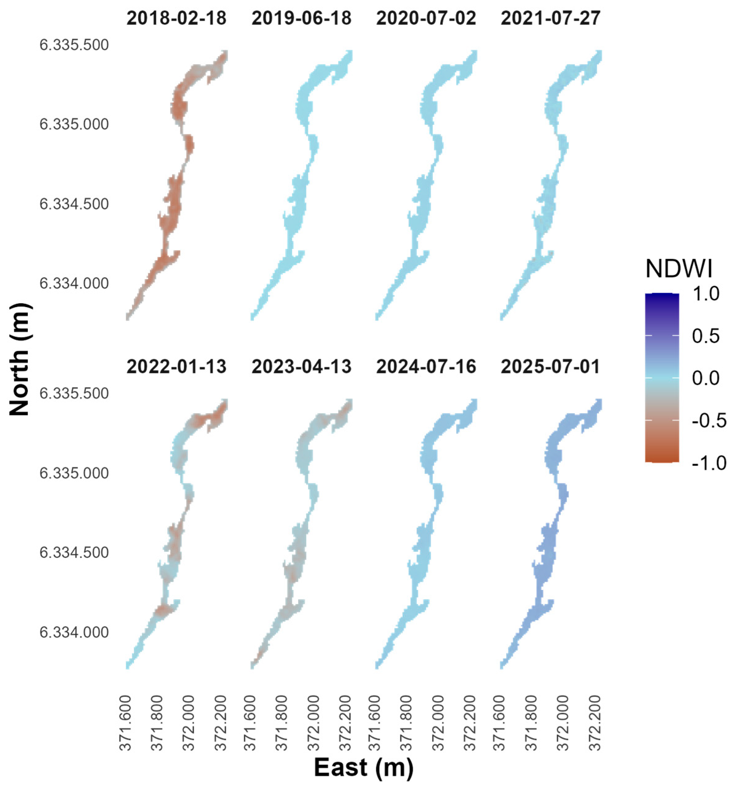
Figure 14.
Multitemporal NDVI color composite for the Lateral wetland (2018–2025), derived from Sentinel-2 imagery acquired during the summer season.
Figure 14.
Multitemporal NDVI color composite for the Lateral wetland (2018–2025), derived from Sentinel-2 imagery acquired during the summer season.
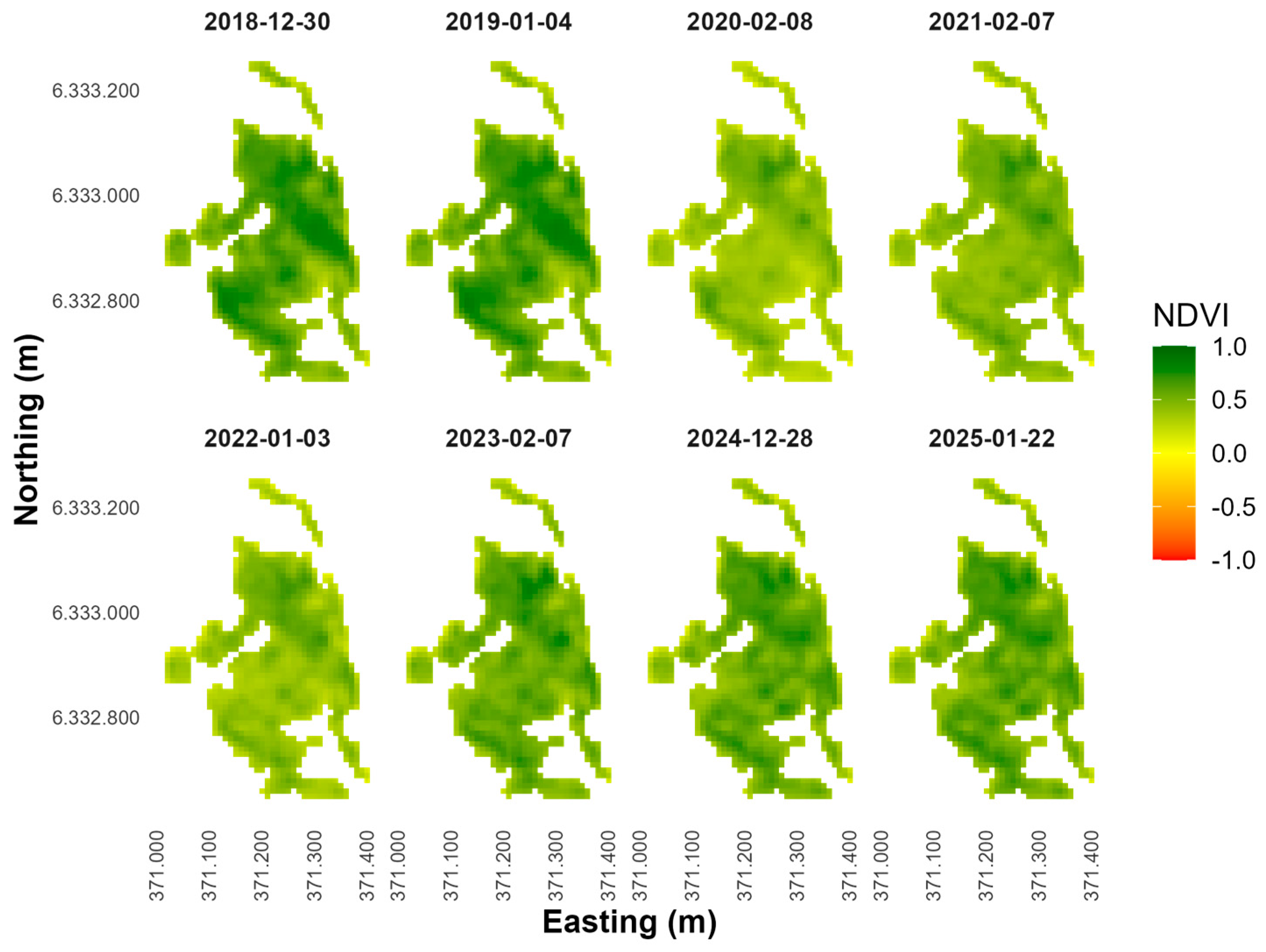
Figure 15.
Multitemporal NDRE705 color composite for the Lateral wetland (2018–2025), showing changes in canopy structure and photosynthetic activity.
Figure 15.
Multitemporal NDRE705 color composite for the Lateral wetland (2018–2025), showing changes in canopy structure and photosynthetic activity.
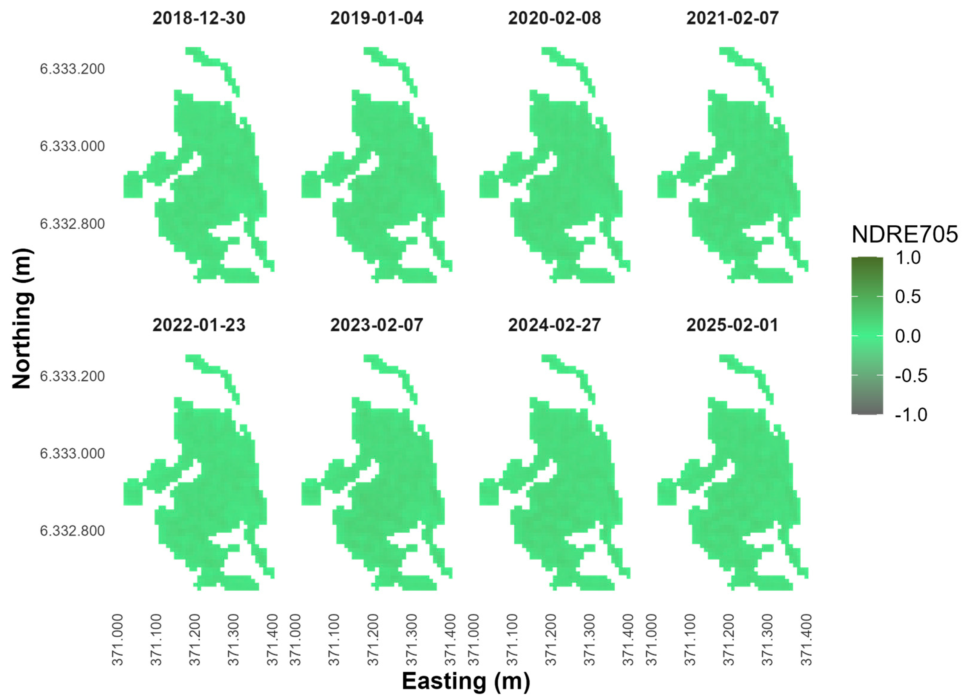
Figure 16.
Multi-temporal EVI mosaic for the Lateral wetland (2018–2025), showing annual variations in vegetation vigor.
Figure 16.
Multi-temporal EVI mosaic for the Lateral wetland (2018–2025), showing annual variations in vegetation vigor.
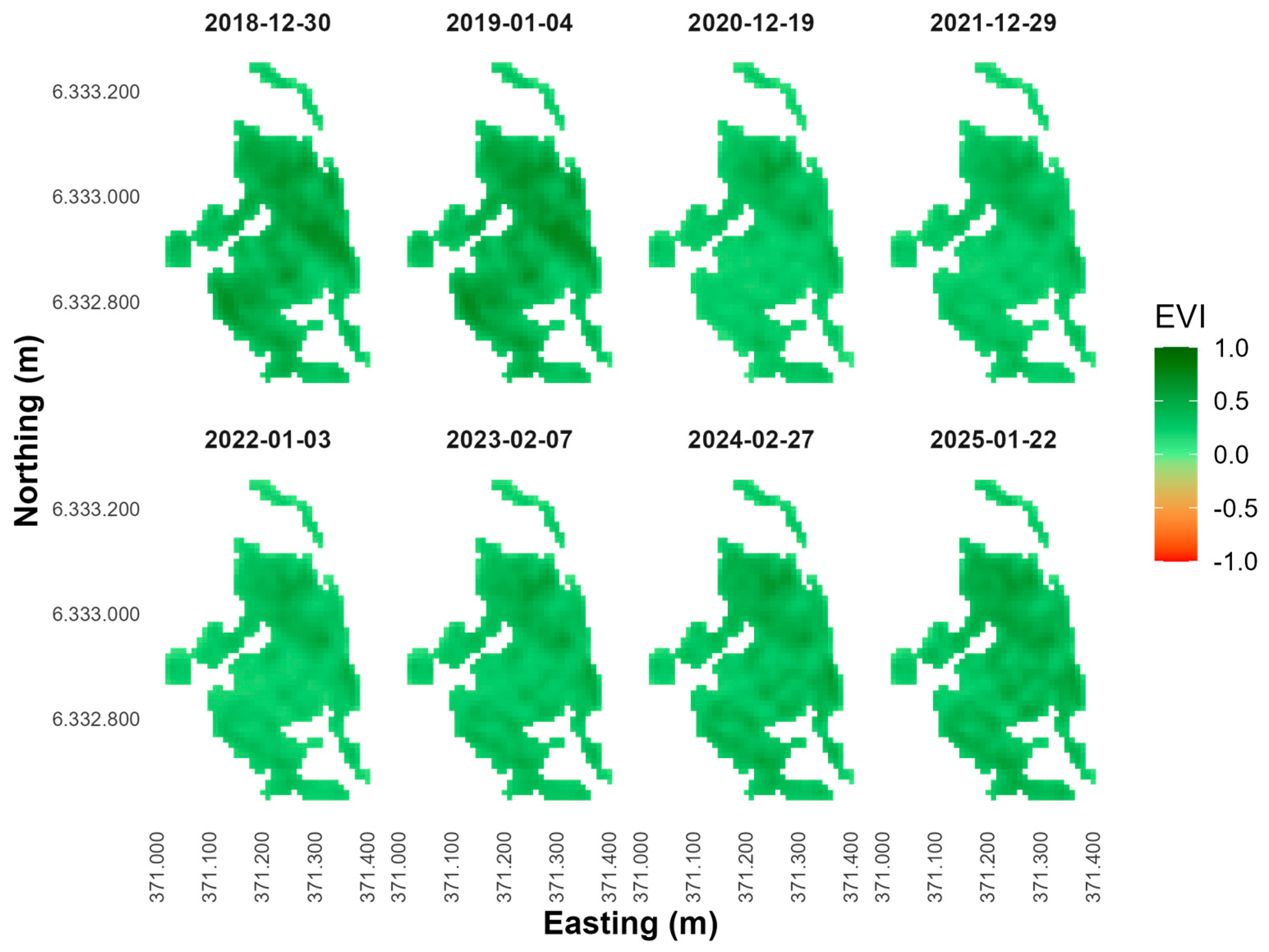
Figure 17.
Multitemporal EVI color composite for the Confluence wetland (2018–2025), showing annual variations in vegetation vigor.
Figure 17.
Multitemporal EVI color composite for the Confluence wetland (2018–2025), showing annual variations in vegetation vigor.
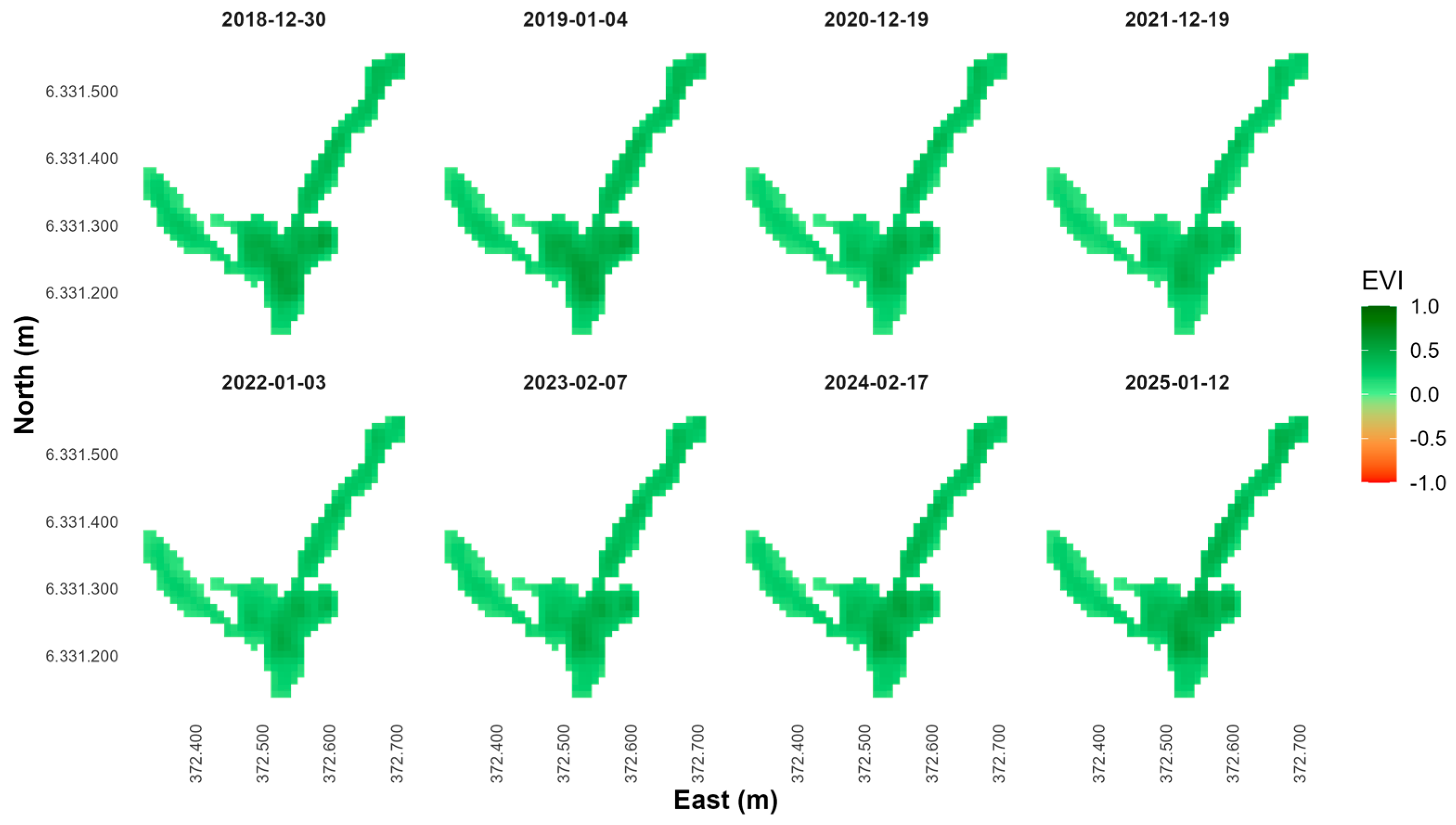
Figure 18.
Multitemporal NDRE704 color composite for the Confluence wetland (2018–2025), representing spatial and temporal variations in chlorophyll concentration.
Figure 18.
Multitemporal NDRE704 color composite for the Confluence wetland (2018–2025), representing spatial and temporal variations in chlorophyll concentration.
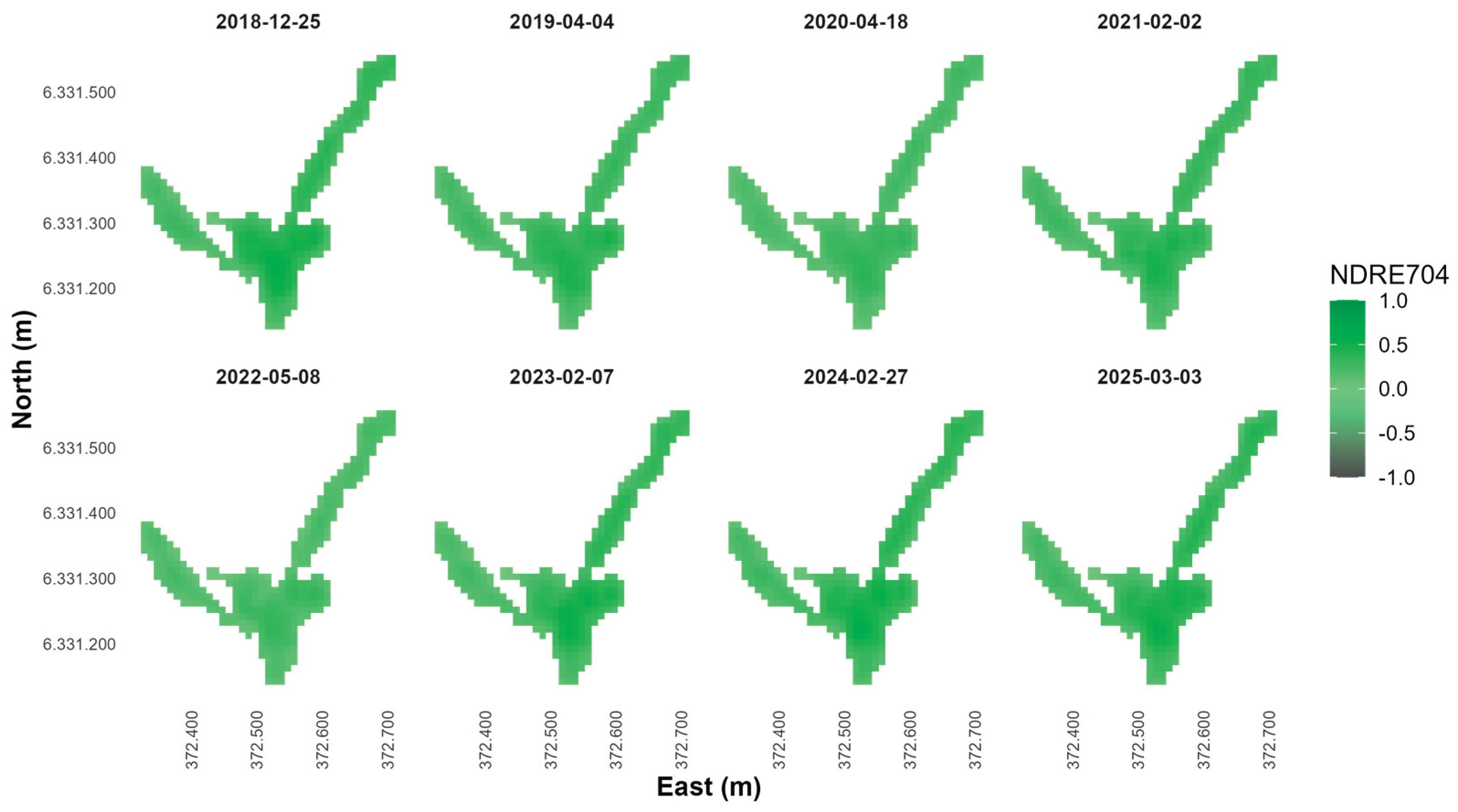

Table 1.
Area of Andean wetland analyzed.
| Wetlands Surface (ha) | |||
|---|---|---|---|
| 1HW | 2LW | 3CW | Total Surface |
| 9.17 | 8.18 | 2.14 | 19.49 |
Table 2.
Spectral indices used in the study, Sentinel-2 and UAV bands, and references.
| Index | Equation | Sentinel-2 Bands | Main purpose | Reference |
|---|---|---|---|---|
| NDVI | (B8 – B4) / (B8 + B4) | B8 (NIR – 842 nm), B4 (Red – 665 nm) | Evaluates vegetation vigor and productivity. | [10] |
| EVI | 2.5 × (B8 – B4) / (B8 + 6×B4 – 7.5×B2 + 1) | B8 (NIR– 842 nm), B4 (Red – 665 nm), B2 (Blue – 490 nm) | Enhances sensitivity in high biomass areas and reduces atmospheric effects. | [11] |
| NDRE704 | (B8 – B5) / (B8 + B5) | B8 (NIR– 842 nm), B5 (Red Edge 1 – 704 nm) | Detects variations in chlorophyll content and foliar stress. | [12] |
| NDRE705 | (B8 – B6) / (B8 + B6) | B8 (NIR– 842 nm), B6 (Red Edge 2 – 705 nm) | Evaluates early physiological conditions of the canopy. | [13] |
| NDWI | (B8 – B11) / (B8 + B11) | B8 (NIR– 842 nm), B11 (SWIR – 1610 nm) | Estimates canopy and surface soil moisture. | [15] |
| SAVI | (1.5 × (B8 – B4)) / (B8 + B4 + 0.5) | B8 (NIR– 842 nm), B4 (Red – 665 nm) | Corrects soil background effects in areas with low vegetation cover. | [17] |
Table 3.
Statistical metrics used in the correlation analysis.
| Metric | Equation | Description and Interpretation | Reference |
|---|---|---|---|
| Pearson correlation coefficient (R) | R = Σ[(xᵢ − x̄)(yᵢ − ȳ)] / √[Σ(xᵢ − x̄)² × Σ(yᵢ − ȳ)²] | Measures the strength and direction of the linear relationship between the previous-year precipitation (x) and the average summer vegetation index (y). Values near 1 or −1 indicate a strong correlation. | [38] |
| Coefficient of determination (R²) | R² = 1 − [Σ(yᵢ − ŷᵢ)² / Σ(yᵢ − ȳ)²] | Indicates the proportion of variance in y explained by x under a linear model. Values close to 1 indicate high explanatory power. | [40] |
| Root Mean Square Error (RMSE) | RMSE = √[(1/n) × Σ(yᵢ − ŷᵢ)²] | Quantifies the average magnitude of residuals (in the same units as y). Lower RMSE indicates better model performance. | [39] |
| Mean Absolute Error (MAE) | MAE = (1 / n) × Σ | yi − ŷi | | The Mean Absolute Error (MAE) represents the average of the absolute differences between observed (yi) and predicted (ŷi) values. It reflects the mean magnitude of prediction errors, regardless of their direction (overestimation or underestimation). | [36] |
| p-value | t = [R × √(n − 2)] / √(1 − R²), t ~ t(n−2) | Tests the null hypothesis H₀: β₁ = 0 in the model y = β₀ + β₁x + ε. A p < 0.05 indicates a statistically significant correlation. | [41] |
Table 4.
Linear regression metrics between previous-year annual precipitation and summer vegetation indices for each wetland. Statistically significant values (p < 0.05) are marked with an asterisk (*).
Table 4.
Linear regression metrics between previous-year annual precipitation and summer vegetation indices for each wetland. Statistically significant values (p < 0.05) are marked with an asterisk (*).
| Wetland | Vegetation index | Slope | R | R2 | RMSE | MAE | p-value |
|---|---|---|---|---|---|---|---|
| Headwater wetland (1HW) | EVI | 0.00026 | 0.72 | 0.52 | 0.04 | 0.03 | 0.04* |
| NDRE704 | 0.00002 | 0.66 | 0.43 | 0.00 | 0.00 | 0.08 | |
| NDRE705 | 0.00025 | 0.79 | 0.62 | 0.03 | 0.02 | 0.02* | |
| NDVI | 0.00040 | 0.79 | 0.63 | 0.04 | 0.04 | 0.02* | |
| NDWI | -0.00025 | -0.80 | 0.63 | 0.03 | 0.02 | 0.02* | |
| SAVI | 0.00022 | 0.70 | 0.50 | 0.03 | 0.03 | 0.05* | |
| Lateral wetland (2LW) | EVI | 0.00020 | 0.52 | 0.27 | 0.05 | 0.04 | 0.18 |
| NDRE704 | -0.00001 | -0.18 | 0.03 | 0.01 | 0.01 | 0.67 | |
| NDRE705 | 0.00019 | 0.60 | 0.36 | 0.03 | 0.02 | 0.12 | |
| NDVI | 0.00025 | 0.59 | 0.35 | 0.05 | 0.04 | 0.12 | |
| NDWI | -0.00009 | -0.35 | 0.12 | 0.03 | 0.03 | 0.40 | |
| SAVI | 0.00013 | 0.43 | 0.19 | 0.04 | 0.03 | 0.28 | |
| Confluence wetland (3CW) | EVI | 0.00010 | 0.56 | 0.32 | 0.02 | 0.02 | 0.15 |
| NDRE704 | -0.00004 | -0.48 | 0.23 | 0.01 | 0.01 | 0.23 | |
| NDRE705 | 0.00005 | 0.22 | 0.05 | 0.03 | 0.02 | 0.61 | |
| NDVI | 0.00007 | 0.19 | 0.04 | 0.05 | 0.04 | 0.64 | |
| NDWI | 0.00006 | 0.15 | 0.02 | 0.06 | 0.04 | 0.73 | |
| SAVI | 0.00002 | 0.07 | 0.00 | 0.03 | 0.02 | 0.87 |
Disclaimer/Publisher’s Note: The statements, opinions and data contained in all publications are solely those of the individual author(s) and contributor(s) and not of MDPI and/or the editor(s). MDPI and/or the editor(s) disclaim responsibility for any injury to people or property resulting from any ideas, methods, instructions or products referred to in the content. |
© 2025 by the authors. Licensee MDPI, Basel, Switzerland. This article is an open access article distributed under the terms and conditions of the Creative Commons Attribution (CC BY) license (http://creativecommons.org/licenses/by/4.0/).
Copyright: This open access article is published under a Creative Commons CC BY 4.0 license, which permit the free download, distribution, and reuse, provided that the author and preprint are cited in any reuse.


