
Submitted:
01 December 2025
Posted:
02 December 2025
You are already at the latest version
Abstract
Deer–vehicle collisions (DVCs) are a persistent safety and economic concern in Pennsylvania, yet quantitative tools for identifying high-risk locations at the road-segment scale remain limited. This study develops a Bayesian spatiotemporal modeling framework for DVCs on state-maintained roads, using PennDOT Public Crash Data linked to the State Road Segment (RMSSEG) inventory. Police- and driver-reported crashes from 2018–2024 were geocoded and matched to homogeneous state road segments, then aggregated to segment–quarter counts. Segment-level covariates included total paved width, lane count, an ordinal urban–rural classification, and annual average daily traffic (AADT), which entered the model as an exposure offset. Exploratory analysis showed that DVCs are rare and highly zero-inflated at the segment–quarter level, exhibit a stable seasonal pattern with peaks in the fourth quarter, and increase monotonically with traffic volume. We modeled DVC counts using negative binomial (NB) mixed-effects models with a shared log-linear predictor incorporating BYM2 spatial random components, a first-order temporal random walk, and an optional quarterly seasonal component. Model estimation utilized INLA, with performance assessed through DIC, WAIC, mean absolute deviance, and mean squared prediction error metrics. The NB specification including quarterly seasonality significantly outperformed an equivalent model lacking seasonal terms, while coefficient estimates for fixed effects showed consistency across models. The NB size parameter indicated strong overdispersion, and the BYM2 mixing parameter suggested that roughly 90% of residual spatial variance is structured along the segment adjacency graph. Comparison of empirical and model-based zero proportions showed that the NB model with spatiotemporal random effects adequately reproduced the extreme sparsity, making a zero-inflated NB specification unnecessary. Out-of-sample validation for 2024 demonstrated low bias and good predictive performance, and risk stratification revealed that a small fraction of highway corridors accounts for a disproportionate share of observed DVCs. The proposed framework provides a practical tool for generating seasonal DVC risk maps and prioritizing corridor-level mitigation measures such as wildlife fencing, crossing structures, and targeted speed management.
Keywords:
deer–vehicle collisions
; negative binomial regression
; BYM2 spatial model
; integrated Nested Laplace Approximation (INLA)
; roadway segment risk
Bayesian Spatial-Temporal Modeling of Deer–Vehicle Collisions on State Roads: A Segment-Level Analysis in Pennsylvania
Deer–vehicle collisions (DVCs) represent a persistent public safety and environmental concern across the United States. A DVC refers to any motor vehicle crash involving a deer, either through a direct impact (vehicle strikes a deer) or indirect involvement (a vehicle swerves to avoid a deer and hits another object or vehicle). These incidents form a major subset of wildlife–vehicle collisions (WVCs) and often result in substantial human injury, property damage, and ecological disruption.
Pennsylvania, with its extensive rural road network and high deer population density, consistently ranks among the states with the highest number of deer-related crashes. In 2023, the Pennsylvania Department of Transportation (PennDOT) reported 6,315 deer-related crashes, resulting in 1,223 injuries and 23 fatalities (Pennsylvania Department of Transportation, n.d.). The Northwest region alone recorded 545 DVCs, including four fatalities, underscoring the need for targeted mitigation. Nationally, more than one million large-animal collisions occur annually, with an estimated cost of $8.4 billion in damages, injuries, and cleanup (Huijser et al., 2007).
DVCs exhibit pronounced temporal and spatial patterns that are closely tied to deer behavior and environmental context. A strong seasonal peak typically occurs in autumn, particularly October and November, corresponding to the deer breeding season and associated increases in movement and dispersal (Seiler, 2004). Time of day is also critical: most animal–vehicle collisions occur at dawn and dusk when deer are most active and driver visibility is reduced (Sullivan, 2009). Recent work using Bayesian space–time interaction models in Minnesota has shown that incorporating temporal dynamics can substantially improve the identification of evolving DVC hotspots (Ashraf & Dey, 2022).
A large body of research has documented how environmental and roadway factors influence DVC risk. Forested areas, agricultural fields, wetlands, and transitional “edge” habitats are positively associated with collision frequency, particularly where roads traverse these landscapes in rural settings (Gunson et al., 2011). Road design characteristics such as number of lanes, horizontal and vertical alignment, grade-separated intersections, and highway corridors have been shown to affect deer movement and collision likelihood (Bhattarai, 2024; Acharya, 2022). Traffic volume is a strong predictor of DVCs, but its effect often interacts with land cover and road type, complicating simple linear interpretations (Hedlund et al., 2004; Knapp, 2005). These findings motivate the inclusion of both road design and spatial layout as key covariates in predictive models.
Mitigation strategies range from infrastructure-based to behavioral interventions. Active measures such as fencing and wildlife overpasses are highly effective but expensive, whereas passive measures like static warning signs are cheaper but tend to lose effectiveness over time (Putman, Langbein, & Staines, 2004). More recent studies suggest that dynamic warning systems—such as motion-activated or seasonal signage—can improve driver awareness and reduce collisions (Khalilikhah & Heaslip, 2017). Driver perception is also critical: Riley and Marcoux (2006) found that many motorists lack basic knowledge about deer behavior and crash risk, highlighting the importance of public education.
Taken together, prior research indicates that DVCs arise from interacting temporal, environmental, and roadway factors. Building on these insights, the present study focuses on temporal patterns and spatial variation across roadway segments in Pennsylvania, using detailed crash and roadway data to develop a segment-level prediction model for deer-related vehicle crashes that can support targeted, corridor-level risk mitigation.
Literature Review
Modeling Approaches
Accurate crash prediction at the roadway segment level is essential for transportation safety planning, allowing agencies to proactively target high-risk areas for intervention. Research in this area has evolved from traditional generalized linear models (GLMs) to more flexible approaches that account for the complex and heterogeneous nature of crash data.
Classical Statistical Model
Early studies frequently employed Poisson regression, which assumes crash counts follow a Poisson distribution with equal mean and variance. Ma (2006) modeled traffic crash counts simultaneously at different severity levels for a given roadway segment using multivariate Poisson–lognormal (MVPLN) models, thereby highlighting the central role of the Poisson framework in crash count modeling. However, overdispersion, where the variance exceeds the mean, which is common in crash data, leading to the adoption of Negative Binomial (NB) models (Lord & Mannering, 2010). NB models have become the standard for segment-level crash modeling due to their ability to handle overdispersal data. However, NB models assume homogeneous effects and are not well-suited for data with excess zeros, which is common in rural deer-related crashes, limiting their effectiveness in capturing spatial and behavioral heterogeneity across segments. To address the prevalence of zero-crash segments, researchers have employed zero-inflated and hurdle models, such as the Zero-Inflated Negative Binomial (ZINB) and Hurdle NB. For example, Shiyuka (2018) found that hurdle models were suitable for overdispersed and zero-heavy crash counts in Namibia. However, ZINB and Hurdle models still struggle to capture unobserved heterogeneity and fail to fully account for spatial and temporal variation.
Random Effects and Mixed Models
Segment-level crash data often exhibit unobserved heterogeneity, arising from differences in traffic conditions, driver behavior, or local environmental factors. To account for this, random-effects and mixed-effects NB models have been used.
Ma et al. (2017) demonstrated that random-effects models enhance crash prediction accuracy on expressways by accounting for unobserved heterogeneity at the segment level. Tang et al. (2021) applied ZINB models with random parameters to tunnel segments, capturing both excess zeros and unobserved heterogeneity. Stapleton et al. (2019) employed mixed-effects negative binomial models to analyze deer–vehicle collisions, highlighting the significance of roadway geometry, land cover, and traffic flow as predictive covariates. However, their modeling framework did not analyze at segment level, limiting its ability to capture space-dependent variation in crash risk.
Spatial and Spatiotemporal Models
Building on these aspatial count models, researchers have increasingly incorporated spatial structure to account for the geographic nature of crash occurrence. Miaou et al. (2003) demonstrated that space–time modeling within a Bayesian hierarchical framework is a powerful approach for analyzing traffic crash data. Since deer-related crash occurrences are strongly location-dependent, spatial correlation must be addressed explicitly. Bayesian hierarchical models with spatial random effects and spatial autoregressive models have therefore been used to capture dependence across neighboring roadway segments or areas. For example, Aguero-Valverde and Jovanis (2008) applied full Bayesian Poisson–lognormal models with conditional autoregressive (CAR) spatial effects to rural two-lane segments in Pennsylvania and showed that accounting for spatial correlation substantially improved model fit and altered key covariate effects, particularly those associated with AADT. Zeng et al. (2017) further extended this line of work by proposing a Bayesian spatial Tobit model with random parameters that effectively captured both spatial correlation and zero inflation in crash counts.
Spatiotemporal models have also been developed to examine how crash risk evolves jointly over time and space. Wen et al. (2019), for instance, introduced a Bayesian spatiotemporal model based on a Poisson–lognormal framework with CAR priors for spatial random effects and temporal autoregressive components. Their model was used to assess the main and interaction effects of roadway geometry (e.g., slope) and adverse weather on crash risk, illustrating how spatiotemporal structures can disentangle persistent spatial patterns from temporal dynamics in crash occurrence. However, these models did not account for other geometric features such as lane width, number of lanes, or their interactions with weather conditions, which will be incorporated in the deer-related crash prediction model developed in the present study.
Machine Learning Approaches
Recent studies have leveraged machine learning (ML) for crash prediction, particularly when datasets contain nonlinear relationships and high-dimensional features. Algorithms such as Random Forests, Gradient Boosting (e.g., XGBoost), optimized radial basis function neural networks (RBFNNs), and Support Vector Machines have shown strong predictive performance in general crash modeling applications (Shanthi et al., 2011; Xie et al., 2007; Huang et al., 2016; Iranmanesh et al., 2022). However, these models are often criticized for limited interpretability, which can hinder their use in transportation policy and engineering practice where understanding covariate effects is as important as prediction accuracy.
To address this limitation, several authors have proposed hybrid or explainable ML frameworks. For example, Zeng et al. (2016) combined artificial neural networks with rule extraction techniques to recover decision rules underlying the trained network. Although promising, such approaches have not yet been widely applied to deer-specific crash prediction. In the context of wildlife–vehicle collisions, Bell et al. (2024) used SMOTE and ensemble ML methods to mitigate class imbalance and reported improved predictive performance for wildlife–vehicle collision risk. Their study illustrates the potential of ML for handling highly imbalanced data, but the models do not explicitly incorporate seasonal or regional random effects. As a result, it is difficult to disentangle whether improvements in accuracy stem from a better representation of temporal and spatial heterogeneity or from the flexible, potentially overfitting nature of ensemble algorithms.
Given these considerations, and our primary interest in quantifying the effects of roadway, traffic, and urban–rural context while explicitly modeling spatial and temporal dependence, the present study adopts an interpretable Bayesian spatiotemporal negative binomial framework rather than a purely machine-learning approach. ML-based models can be viewed as complementary tools for future work, particularly for exploring nonlinearities once the key structural relationships are established.
Data
The analysis focuses exclusively on deer-related vehicle collisions occurring on state-managed roads in Pennsylvania. The primary datasets include PennDOT's Public Crash Data and the State Road Segment dataset (RMSSEG). The dataset spans the years 2018 through 2024 will be used for analysis.
Crash Data
This study relies on publicly available crash data published by the Pennsylvania Department of Transportation (PennDOT) annually through its Public Crash Data portal. The crash records are compiled from three primary sources: Police-Reported Crash Reports, Driver-Reported Crash Reports (Form AA-600) and Calculated and Derived Fields from CDART. Most crash data come from standardized crash reports submitted to PennDOT by law enforcement agencies across the state. Police officers investigating a crash complete detailed records using the state-standard reporting protocol. These reports capture comprehensive information, including crash location, vehicle movements, environmental conditions, and observed contributing factors such as speeding or deer presence. For minor crashes not investigated by police, Pennsylvania drivers can submit self-reported crash information using Form AA-600, also known as the Driver’s Accident Report form. These entries supplement police reports but are less detailed and not used when police documentation is already available. PennDOT maintains a centralized database known as the Crash Data Analysis and Retrieval Tool (CDART). This system aggregates raw reports from police and drivers, applies data validation rules, and computes additional derived variables. These derived fields may include time-of-day categorization, severity classifications, and spatial attributes (e.g., county and district codes), ensuring consistency across the dataset. Only non-sensitive variables are included in the Public Crash Data Files, which are structured into eight normalized CSV tables. For this study, three key tables were utilized: CRASH, FLAG, and ROADWAY. These are linked using the Crash Record Number (CRN), a unique identifier assigned to each crash event.
Segment Data
State Roads Segment Data (RMSSEG) provides the official segmentation of Pennsylvania's state-maintained roadway network, derived from PennDOT’s Roadway Management System (RMS), which divided roadways into homogeneous segments. Begin/end mile points for each segment are based on a change in one or more primary characteristics, including pavement surface, annual average daily traffic, major junction, jurisdictional boundary, and numerous other features, and provided the roadway segmentation basis for data collected during this study. The shapefile was used to provide the spatial basis for collection of the necessary roadway and traffic related attributes. The file represents a digital base map for the state, consisting of all public road segments, in addition to census boundaries and other relevant geographic boundaries and other spatial characteristics across PA.
Each line segment includes route details, segment identifiers, and attributes such as: County, District, Route Number, Segment & Offset, Functional Class, Number of Lanes, Speed Limit, Urban/Rural designation, Median Type, Annual Average Daily Traffic values and Spatial geometry for mapping in GIS. Each segment is associated with an engineering length. A unique segment can be identified by concatenated country code, street route number and segment number.
Explanatory Variables
We analyzed police-reported deer–vehicle collisions (DVCs) on state-maintained roads. We obtained a road inventory containing segment-level characteristics, including Segment ID (unique identifier combining county, route, and segment); Total paved width (sum of lane and shoulder widths); Number of lanes; Urban–rural classification (1 = Rural Area (Non-CDP, Non-City), 2=Census Designated Place (CDP), 3=Incorporated Village / Borough,4=Incorporated City); AADT (Annual average daily traffic). Additional variables such as speed limit, segment length or roughness index were considered during preliminary analysis but are not included in the final comparative model set to streamline interpretation and reduce dimensionality.
Spatiotemporal Aggregation
Using latitude and longitude, which are numerical variables representing the exact crash coordinates and are essential for GIS mapping and spatial joins, crash records were linked to a segmented road inventory based on the nearest location. Records without valid segment references or with missing coordinates that could not be confidently matched were excluded from the analysis to avoid misallocation. For each unique road segment and calendar quarter, we computed the total number of DVCs and merged this with segment-level roadway attributes. To capture temporal patterns, crashes were aggregated to segment–quarter units. For each segment and quarter , we computed the count of deer-related crashes, . Quarters were indexed from 1 to 4 within a year and extended across years via a continuous index. Segment-level covariates (total width, lane count, urban–rural status) were treated as time-invariant over the study period. AADT was assumed constant within year and used as an exposure measure via an offset term.
Continuous covariates were standardized (mean 0, SD 1) to aid interpretation and numerical stability. The final dataset consisted of all segments–quarter combinations over the analysis period, including segment–quarter units with zero observed DVCs, ensuring that zeros were explicitly modeled rather than excluded.
Exploratory Data Analysis
Exploratory data analysis (EDA) indicated that deer–vehicle collisions (DVCs) are rare events at the roadway segment–quarter level. Over the six-year period from 2018 to 2023, only a small fraction of segments experienced any DVC: 90,227 segments had no recorded DVC during the entire study period, whereas 22,150 segments experienced at least one collision (Figure 1). This extreme sparsity at the segment level is consistent with a highly zero-inflated outcome distribution and motivates the use of overdispersed count models with segment-level random effects. In subsequent analyses, we therefore place particular emphasis on segments with repeated DVCs over the study period, as these locations represent persistent high-risk sites.
Despite the low absolute frequency of events, the quarterly occurrence probability exhibited a highly regular temporal pattern. The proportion of segment–quarters with at least one DVC ranged from approximately 0.6% to 2.5%, but followed a consistent seasonal cycle: minima occurred in the first quarter and maxima in the fourth quarter of every year between 2018 and 2023 (Figure 2). This stability suggests a strong and persistent seasonal component in DVC risk rather than random inter-annual variation.
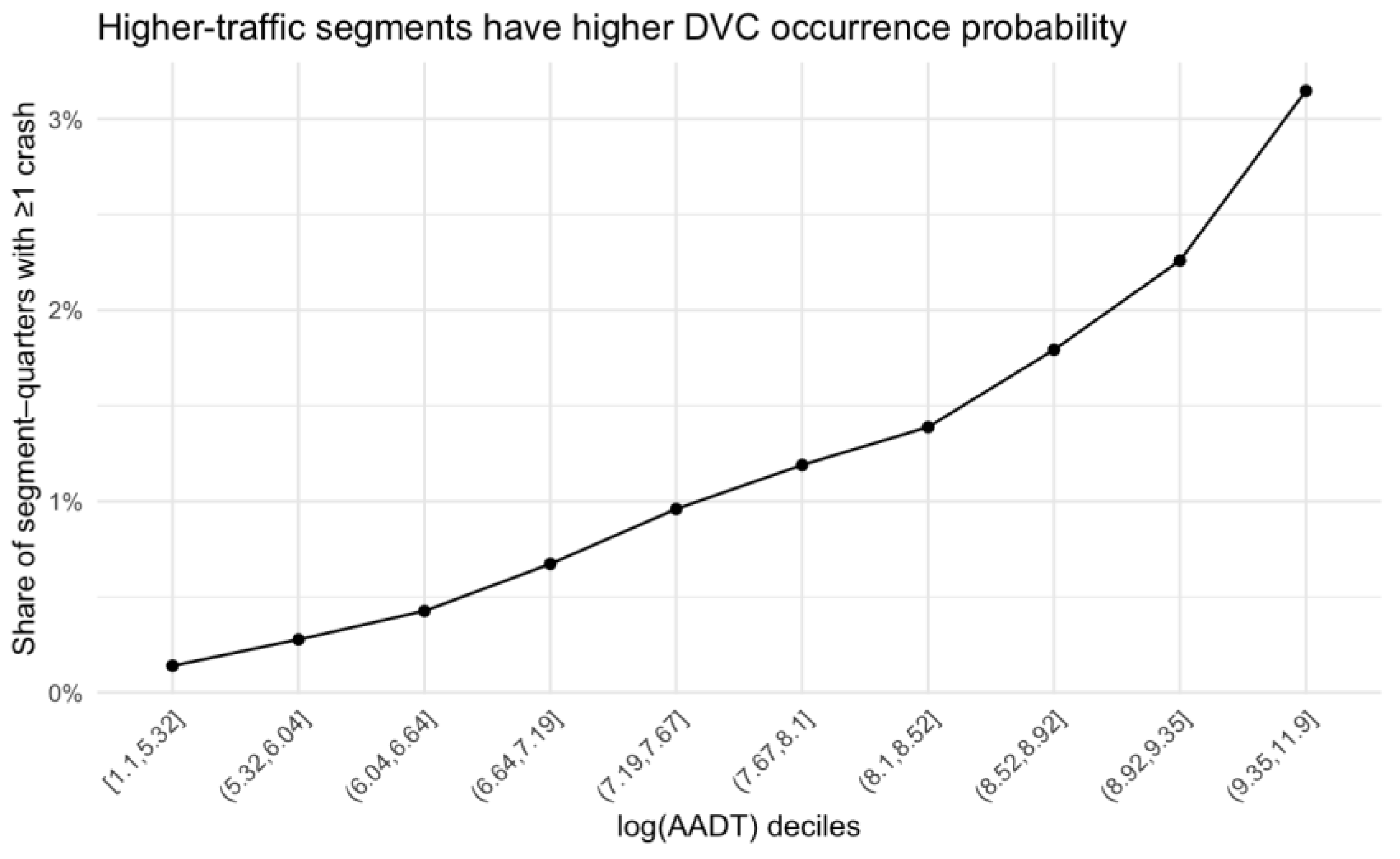
Crash occurrence was also strongly associated with traffic exposure. When segment–quarters were grouped into deciles of log(AADT), the probability of observing at least one DVC increased approximately monotonically with traffic volume (Figure 2b). Segments in the lowest traffic deciles had probabilities below 0.5%, whereas those in the highest decile exceeded 3%. Together, these patterns indicate that DVCs are rare but systematically structured in time and space, with risk concentrated on higher-volume segments and during the late-year (Q4) period.
Figure 3.
Crash occurrence vs traffic volume (log_AADT).
Methods
Models Structure
We modeled the count of deer-related crashes on segment in quarter using negative binomial, or zero-inflated negative binomial if necessary. All models shared the same linear predictor and random-effects structure.
Let denote the crash count and the mean crash rate. The general predictor was:
Random Effects
Seasonal Random Effect
was modeled with a seasonal structure of period 4:
Spatial Random Effects
Road segments that are close to each other may share similar unobserved conditions, such as lighting, pavement condition, roadside vegetation, and other environmental factors—that affect deer–vehicle collision (DVC) risk. If this spatial correlation is ignored, regression coefficients can be biased and uncertainty underestimated (Zeng and Huang, 2014). To account for this, was modeled using a BYM2 (Besag–York–Mollié 2) specification based on a segment adjacency graph.
Let represent the combined spatial random effect for segment . In the BYM2 parameterization,
are i.i.d. unstructured random effects.
follow an intrinsic conditional autoregressive (ICAR) model based on the road-segment adjacency graph.
is a precision parameter controlling overall spatial variability.
is a mixing parameter indicating the proportion of spatial variance attributed to the structured (ICAR) component.
The adjacency structure for the ICAR model is derived from the state road network: two segments are treated as neighbors if they share a common endpoint. When is close to 1, most of the spatial variability is structured according to this adjacency graph (strong spatial clustering); when is close to 0, the spatial variability is dominated by unstructured noise. This BYM2 formulation separates the total spatial variance (controlled by ) from the fraction that is spatially structured (controlled by ), improving both identifiability and interpretability of the spatial random effects.
Long-Term Temporal Trend
was modeled as a first-order random walk (RW1) over ordered quarters,
Penalized complexity (PC) priors were assigned to the precision parameters of these random effects and to the BYM2 mixing parameter. Lag-1 implies that the temporal effect on a specific segment in current period is affected by its counterpart in the previous one (quarter in current study).
Distributional Assumptions
There are two general modeling approaches for quartile DVC counts per segment.
Negative binomial (NB) mixed-effects model
Zero-inflated negative binomial (ZINB) mixed-effects model
The same fixed and random effects entered the linear predictor for across all families.
Assessment of Zero Inflation
Prior studies have noted that apparent zero inflation in crash data often diminishes once spatial and other random effects are included, because latent heterogeneity and clustering can generate a large number of zeros without requiring a separate zero-inflation component. To evaluate whether a zero-inflated model was necessary in our setting, we used a post–model-checking approach based on the negative binomial (NB) mixed-effects model.
For the NB model, the theoretical probability of observing zero crashes for a given segment–quarter, conditional on the predicted mean and dispersion parameter (size), is
Goodness-of-Fit Measures
We employed five categories of fit criteria to assess and compare the Bayesian spatial models: (i) information criteria (DIC), (ii) within-sample deviance measures (MAD), and (iii) out-of-sample prediction metrics (MSPE). All models were fitted using Integrated Nested Laplace Approximation (INLA), which directly calculates the deviance information criterion without requiring computationally intensive MCMC sampling, thus eliminating the need for convergence diagnostics.
Deviance Information Criterion (DIC) Following Spiegelhalter et al. (2002), DIC combines posterior mean deviance (measuring model fit) with the effective number of parameters (measuring complexity). Lower DIC values are preferred. DIC differences of 5-10 are considered substantial, while differences exceeding 10 indicate clearly superior performance of the lower-DIC model (Spiegelhalter et al., 2005).
Mean Absolute Deviance (MAD)
To evaluate how closely predicted crash frequencies match the observed values across all spatial-temporal units, the mean absolute deviance is computed as
Mean Squared Prediction Error (MSPE)
For out-of-sample validation, the model’s predictions for each quarter in 2024 were compared against the observed crash counts for the same period. The MSPE is defined as
Lower MAD and MSPE values reflect superior predictive accuracy. The combination of DIC, MAD, and MSPE enables comprehensive assessment of (i) within-sample fit quality, (ii) model complexity and parsimony, and (iii) real-world predictive capability.
Results
Comparison of Negative Binomial Models with and Without Seasonal Effects
We first compared the negative binomial model without seasonal quarter effects and the corresponding model that incorporates a quarterly random effect. As shown in Table 1, the model with quarter effects achieves lower DIC (315,651.70 vs. 315,790.64) and WAIC (315,422.49 vs. 315,494.47), together with a slightly smaller effective number of parameters (11,935.86 vs. 12,040.89). The marginal log-likelihood is also improved (−203,746.27 vs. −203,788.20). These differences, especially the DIC reduction of approximately 139, indicate that the NB model with quarter effects provides a substantially better fit than the NB model that ignores seasonality.
This finding is consistent with the expectation that DVC risk exhibits strong within-year variation, and that explicitly modeling quarter-to-quarter variation can mitigate model misspecification and improve overall fit. Notably, the estimated fixed effects remain very similar across the two models (same sign and comparable posterior means), suggesting that the improvement is primarily due to capturing residual seasonal structure rather than changing the estimated associations between roadway characteristics and DVC frequency.
The inclusion of the seasonal term also alters the temporal random effect. In the model without quarter, the RW1 precision for TIME_KEY_Q is relatively low (mean 1.56; 95% CrI: 1.02–2.32), implying more pronounced long-term fluctuations. After adding the quarter effect, the RW1 precision increases dramatically (mean 669.50; 95% CrI: 307.78–1463.09), indicating that once seasonality is accounted for, the remaining long-term trend is very smooth. In contrast, the spatial BYM2 precision (0.45; 95% CrI: 0.43–0.48) and mixing parameter (Φ ≈ 0.91; 95% CrI: 0.90–0.93) are essentially unchanged between the two models, suggesting that the strength and structure of spatial correlation are robust to the inclusion of seasonal effects. Based on these results, the NB model with quarter effects was selected as the preferred specification for subsequent inference and prediction.
Interpretation of Fixed Effects
Posterior summaries for the fixed effects in the selected NB model with quarter effect reveal strong and interpretable associations between roadway characteristics, urban–rural context, and DVC frequency.
Total Paved Width
The coefficient for standardized total width is negative and statistically significant, with posterior mean
On the rate scale, this corresponds to , indicating that a one-standard-deviation increase in total paved width is associated with an approximate 27% reduction in the expected number of deer-related crashes per segment–quarter, holding other variables and random effects constant. This result suggests that wider cross-sections may provide better lateral clearance, improved sight distance, and more recovery space for drivers, thereby reducing the likelihood of collisions with deer.
Lane Count
In contrast, the coefficient for standardized lane count is positive:
Urban–Rural Status
The urban–rural classification was coded on a four-level ordinal scale (1 = Rural Area [Non-CDP, Non-City], 2 = Census Designated Place [CDP], 3 = Incorporated Village / Borough, 4 = Incorporated City), and then standardized before modeling. The estimated coefficient for this standardized index is
Intercept
The intercept (−12.95; 95% CrI: −13.18, −12.73) reflects the log collision rate for a segment with average covariate values (after standardization), average quarter, and baseline random effects, at the reference level of AADT. Its large negative value highlights the extremely low baseline probability of a DVC per segment–quarter in the absence of risk-enhancing conditions
Overdispersion and Random Effect’s Structure
The negative binomial size parameter in the chosen model is
The spatial BYM2 component exhibits strong structured residual variation, with precision of 0.45 (95% CrI: 0.43–0.48) and mixing parameter
These estimates imply that approximately 90% of the residual spatial variance is accounted for by the structured component defined over the road-segment adjacency graph. In other words, neighboring segments tend to share similar unexplained risk levels even after controlling for traffic exposure, roadway geometry, and urban–rural status. Such spatial clustering is likely driven by unmeasured or imperfectly measured factors (e.g., local deer habitat, roadside vegetation, micro-topography, and lighting conditions) that vary systematically along the network.
The seasonal quarter effect has a precision of 3.47 (95% CrI: 1.41–8.68), confirming the presence of notable within-year variability in DVC risk. Meanwhile, the very high precision of the RW1 temporal effect once the seasonal term is included suggests that the remaining long-term trend is smooth and of relatively small magnitude compared with the seasonal and spatial components.
Assessment of Zero Inflation
Finally, we assessed whether an explicit zero-inflated negative binomial (ZINB) specification was required. The empirical proportion of segment–quarter observations with zero DVCs is 0.98637. Using the fitted NB model with quarter effects, the theoretical zero probability for each segment–quarter was computed as
The near equality between the empirical and model-based zero proportions (0.98637 vs. 0.98660) demonstrates that the negative binomial model, combined with spatial and temporal random effects and seasonal quarter effects, already reproduces the extreme sparsity of the data. In light of this close agreement and given the additional complexity and numerical instability associated with the ZINB specification, an explicit zero-inflation component is not warranted. Therefore, the NB model with quarter effects is adopted as the final model for inference and scenario analysis.
Predictive Performance and Risk Stratification
Quarter-specific predictive diagnostics indicate that the NB model with quarter effect achieves accurate out-of-sample predictions with essentially no systematic bias. For quarters Q1–Q4, the mean prediction bias is close to zero (on the order of ), while mean squared prediction error (MSPE) remains modest, with somewhat larger error in Q4 reflecting higher seasonal variability:
Q1: MAD = 0.00035, MSPE = 0.00773
Q2: MAD = 0.00035, MSPE = 0.00773
Q3: MAD = 0.00031, MSPE = 0.00970
Q4: MAD = 0.00002, MSPE = 0.02920
To examine how well the model captures high-risk segments, we grouped RMSSEG segments into five risk classes based on the posterior mean predicted crash count for Q4 2024: 0–0.2, 0.2–0.4, 0.4–0.6, 0.6–0.9, and ≥0.9 crashes per segment–quarter (Table 2). Mean observed crash frequency and the proportion of segments experiencing at least one crash generally increase with predicted risk. For example, segments in the lowest class (0–0.2) have a mean observed rate of 0.0249 crashes and 2.37% non-zero outcomes, whereas segments in the highest class (≥0.9) have a mean observed rate of 1.12 crashes and 75% non-zero outcomes. This monotonic pattern, despite some instability in the upper classes due to small sample sizes, indicates that the model effectively concentrates observed high-risk outcomes into relatively few segments with elevated predicted risk.
Discussion
Figure 4 displays the posterior mean predicted DVC rate for each RMSSEG segment, classified into five risk categories (0–0.2, 0.2–0.4, 0.4–0.6, 0.6–0.9, and >0.9 crashes per segment–quarter). Because most segments fall into the lowest class (0–0.2), segments in this class are not plotted in Figure 4 to improve visual contrast. The figure therefore shows only segments with predicted means ≥0.2, colored as dark green (0.2–0.4), purple (0.4–0.6), black (0.6–0.9), and red (>0.9). Even after omitting the lowest-risk class, high predicted risks (0.6–0.9 and >0.9) remain concentrated along a limited number of continuous corridors, primarily high-speed facilities that connect major urban areas and traverse rural or forested landscapes. This corridor-like pattern is consistent with the strong structured spatial effect estimated by the BYM2 component and supports the interpretation that unobserved risk factors are spatially clustered along certain inter-urban routes rather than randomly distributed across the network.
Figure Y presents a zoomed-in view of the corridor between Harrisburg and Philadelphia, overlaying observed Q4 2024 DVC locations on the same risk map used in Figure X. Most observed crashes fall on segments classified as moderate or high risk (dark green, purple, black, and red), particularly along the inter-city highway corridors, whereas segments in the lowest risk class (0–0.2, not shown) exhibit only sparse events. This spatial pattern corroborates the numerical results in Table 2, where both mean observed crash counts and the proportion of segments with at least one crash increase monotonically with predicted risk class. Together, Figure 4 and Figure 5 indicate that the spatiotemporal negative binomial model not only fits the aggregate data well but also effectively concentrates observed DVC risk into a relatively small subset of the network, making it suitable as a screening tool for prioritizing mitigation.
From a management perspective, these maps highlight that DVC risk is organized into distinct high-risk corridors rather than being uniformly spread across the network. Consequently, countermeasures can be targeted to the black and red segments and, where resources allow, adjacent purple segments—to achieve substantial safety gains with limited investment. In particular, inter-urban highways passing through extensive forest or agricultural areas emerge as natural candidates for wildlife fencing and crossing structures, right-of-way vegetation and habitat management, enhanced nighttime signing and delineation, and seasonal interventions such as temporary speed management, enforcement, and traveler information campaigns during the highest-risk quarters. By explicitly incorporating exposure (AADT), roadway geometry, and urban–rural context, the model also helps distinguish segments where high crash counts primarily reflect heavy traffic from those where local environmental or geometric conditions drive elevated risk, thereby providing a quantitative basis for more targeted and cost-effective DVC mitigation strategies.
Conclusion
This study developed a Bayesian spatiotemporal negative binomial modeling framework to examine deer–vehicle collisions (DVCs) on state-maintained road segments in Pennsylvania. Using segment–quarter crash counts from 2018–2024, we compared alternative count distributions and random-effects structures and evaluated their ability to capture overdispersion, spatial and temporal correlation, and the extreme sparsity of the data. Among the candidate specifications, the negative binomial model with a quarterly seasonal random effect and BYM2 spatial structure provided the best overall fit and predictive performance, while a zero-inflated formulation was not warranted.
The preferred model revealed several consistent and interpretable relationships between roadway characteristics, urban–rural context, and DVC risk. After standardization, total paved width exhibited a strong protective effect: a one–standard deviation increase in width was associated with an approximate 27% reduction in expected DVC counts per segment–quarter. In contrast, a one–standard deviation increases in lane county corresponded to roughly a 28% increase in expected crashes, conditional on width and traffic exposure. The urban–rural index showed a clear negative gradient, with more urbanized segments experiencing substantially lower DVC rates than rural segments. These patterns are plausible given higher deer densities, more suitable habitat, and often higher nighttime speeds in rural environments, and they underscore the importance of focusing mitigation efforts on rural and peri-urban transition zones.
The random effects structure further highlighted the importance of spatial and temporal dependence in DVC data. The negative binomial size parameter confirmed substantial overdispersion relative to the Poisson model. The BYM2 mixing parameter suggested that approximately 90% of residual spatial variance is structured according to the road-segment adjacency graph, indicating that neighboring segments tend to share similar unobserved risk factors, such as deer habitat, roadside vegetation, or lighting. The introduction of a quarter-specific seasonal effect substantially improved model fit and yielded a very smooth long-term temporal trend, consistent with strong within-year seasonality in DVC risk.
Out-of-sample validation using Q4 2024 demonstrated that the model predicts segment-level crash frequencies with negligible bias and modest mean squared prediction error. When segments were grouped into risk classes based on predicted DVC rates, observed crash frequencies and the proportion of non-zero outcomes increased monotonically across classes. High-risk segments represented only a small fraction of the network but accounted for a disproportionate share of observed crashes, suggesting that the model can effectively concentrate mitigation resources on a relatively small subset of road segments with elevated risk.
These findings have several practical implications for DVC management. The proposed modeling framework can be used to generate spatially explicit, seasonally varying risk maps that support the prioritization of countermeasures such as warning signage, vegetation management, fencing, or targeted enforcement. By explicitly accounting for exposure (AADT), roadway geometry, and urban–rural context, the model also helps distinguish sites where high crash counts primarily reflect high traffic volumes from sites where elevated risk arises from local geometric or environmental conditions.
This study has limitations that suggest avenues for future work. First, our covariates are limited to traffic exposure, basic cross-sectional geometry, and a coarse urban–rural classification; we lack direct measures of deer abundance, detailed land cover, lighting, and driver behavior, all of which likely contribute to DVC risk. Second, we approximated urbanization using a four-level ordinal index, which may not fully capture heterogeneity within and across urban and rural areas. Third, although the negative binomial model with seasonal and spatial components performed well, we did not explore more flexible nonlinear or interaction terms, nor did we formally compare the Bayesian framework with machine-learning approaches.
Future research could extend this work by incorporating wildlife and habitat data, high-resolution environmental covariates, and dynamic traffic information, and by integrating the spatiotemporal risk model into cost–benefit analyses of alternative mitigation strategies. Nevertheless, the present study demonstrates that a Bayesian spatiotemporal negative binomial model with seasonal and spatial random effects can successfully characterize DVC risk at the road-segment scale, identify high-risk locations, and provide a quantitative foundation for more targeted and efficient DVC mitigation on state highway networks.
References
- Pennsylvania Department of Transportation. State Roads Segment Data (RMSSEG) [Dataset]. PennShare Open Data Portal. n.d. Available online: https://data.pennshare.opendata.arcgis.com/datasets/d9a2a5df74cf4726980e5e276d51fe8d_0.
- Huijser, M. P.; McGowen, P. T.; Fuller, J.; Hardy, A.; Kociolek, A. Wildlife-vehicle collision reduction study: report to congress (No. FHWA-HRT-08-034). 2007. [Google Scholar]
- Seiler, A. Trends and spatial patterns in ungulate-vehicle collisions in Sweden. Wildlife Biology 2004, 10(4), 301–313. [Google Scholar] [CrossRef]
- Sullivan, J. M. Relationships between lighting and animal-vehicle collisions; University of Michigan, Ann Arbor, Transportation Research Institute, 2009. [Google Scholar]
- Ashraf, M. T.; Dey, K. Application of Bayesian Space-Time interaction models for Deer-Vehicle crash hotspot identification. Accident Analysis & Prevention 2022, 171, 106646. [Google Scholar]
- Gunson, K. E.; Mountrakis, G.; Quackenbush, L. J. Spatial wildlife-vehicle collision models: A review of current work and its application to transportation mitigation projects. Journal of environmental management 2011, 92(4), 1074–1082. [Google Scholar] [CrossRef] [PubMed]
- Bhattarai, S. Factors Influencing Deer-Vehicle Crashes at Grade Separated Intersections: A Case Study of Ohio's Appalachian Region. Master's thesis, Ohio University, 2024. [Google Scholar]
- Acharya, S. Corridors and Deer-Vehicle Collisions Along Missouri Interstate Highways. Master’s thesis, University of Missouri-Columbia, 2022. [Google Scholar]
- Hedlund, J. H.; Curtis, P. D.; Curtis, G.; Williams, A. F. Methods to reduce traffic crashes involving deer: what works and what does not. Traffic injury prevention 2004, 5(2), 122–131, Risk Prediction Mapping of Deer-related Crash in PA. [Google Scholar] [CrossRef]
- Knapp, K. K. Deer-vehicle crash countermeasure toolbox: a decision and choice resource. In Midwest Regional University Transportation Center, Deer-Vehicle Crash Information Clearinghouse; University of Wisconsin-Madison, 2004. [Google Scholar]
- Putman, R.; Langbein, J.; Staines, B. W. Deer and Road Traffic Accidents, a Review of Mitigation Measures: Costs and Cost-effectiveness; Inverness, UK; Scottish Natural Heritage, 2004. [Google Scholar]
- Khalilikhah, M.; Heaslip, K. Improvement of the performance of animal crossing warning signs. Journal of Safety Research 2017, 62, 1–12. [Google Scholar] [CrossRef]
- Riley, S. J.; Marcoux, A. Deer-vehicle collisions: an understanding of accident characteristics and drivers' attitudes, awareness and involvement (No. RC-1475); Michigan. Dept. of Transportation. Construction and Technology Division, 2006. [Google Scholar]
- Ma, J. Bayesian multivariate Poisson-Lognormal regression for crash prediction on rural two-lane highways, 2006.
- Lord, D.; Washington, S. P.; Ivan, J. N. Poisson, Poisson-gamma and zero-inflated regression models of motor vehicle crashes: balancing statistical fit and theory. Accident Analysis & Prevention 2005, 37(1), 35–46. [Google Scholar]
- Shiyuka, N. Hurdle negative binomial model for motor vehicle crash injuries in Namibia. Doctoral dissertation, University of Namibia, 2018. [Google Scholar]
- Ma, X.; Kockelman, K. M.; Damien, P. A multivariate hierarchical Bayesian crash frequency model: Addressing spatial correlation and heterogeneity. Transportation Research Part A: Policy and Practice 2017, 103, 118–129, Risk Prediction Mapping of Deer-related Crash in PA. [Google Scholar]
- Tang, F.; Fu, X.; Cai, M.; Lu, Y.; Zhong, S. Investigation of the factors influencing the crash frequency in expressway tunnels: Considering excess zero observations and unobserved heterogeneity. Ieee Access 2021, 9, 58549–58565. [Google Scholar] [CrossRef]
- Stapleton, S. Y.; Ingle, A.; Gates, T. J. Factors contributing to deer–vehicle crashes on rural two-lane roadways in Michigan. Transportation research record 2019, 2673(10), 214–224. [Google Scholar] [CrossRef]
- Miaou, S. P.; Song, J. J.; Mallick, B. K. Roadway traffic crash mapping: a space-time modeling approach. Journal of transportation and Statistics 2003, 6, 33–58. [Google Scholar]
- Zeng, Q.; Wen, H.; Huang, H.; Abdel-Aty, M. A Bayesian spatial random parameters Tobit model for analyzing crash rates on roadway segments. Accident Analysis & Prevention 2017, 100, 37–43. [Google Scholar] [CrossRef]
- Wen, H.; Zhang, X.; Zeng, Q.; Sze, N. N. Bayesian spatial-temporal model for the main and interaction effects of roadway and weather characteristics on freeway crash incidence. Accident Analysis & Prevention 2019, 132, 105249. [Google Scholar] [CrossRef]
- Aguero-Valverde, J.; Jovanis, P. P. Analysis of road crash frequency with spatial models. Transportation Research Record 2008, 2061(1), 55–63. [Google Scholar] [CrossRef]
- Bhattarai, S. Factors Influencing Deer-Vehicle Crashes at Grade Separated Intersections: A Case Study of Ohio's Appalachian Region. Master's thesis, Ohio University, 2024. [Google Scholar]
- Shanthi, S.; Ramani, R. G. Classification of vehicle collision patterns in road accidents using data mining algorithms. International Journal of Computer Applications 2011, 35(12), 30–37. [Google Scholar]
- Xie, Y.; Lord, D.; Zhang, Y. Predicting motor vehicle collisions using support vector machine models. Accident Analysis & Prevention 2007, 39(5), 874–886. [Google Scholar]
- Huang, H.; Zeng, Q.; Pei, X.; Wong, S. C.; Xu, P. Predicting crash frequency using an optimised radial basis function neural network model. Transportmetrica A: transport science 2016, 12(4), 330–345. [Google Scholar] [CrossRef]
- Iranmanesh, M.; Seyedabrishami, S.; Moridpour, S. Identifying high crash risk segments in rural roads using ensemble decision tree-based models. Scientific reports 2022, 12(1), 20024. [Google Scholar] [CrossRef]
- Zeng, Q.; Huang, H.; Pei, X.; Wong, S. C.; Gao, M. Rule extraction from an optimized neural network for traffic crash frequency modeling. Accident Analysis & Prevention 2016, 97, 87–95. [Google Scholar] [CrossRef]
- Bell, M.; Wang, Y.; Ament, R. Risk mapping of wildlife–vehicle collisions across the state of Montana, USA: a machine-learning approach for imbalanced data along rural roads. Transportation Safety and Environment 2024, 6(3), tdad043. [Google Scholar] [CrossRef]
Figure 1.
2018-2023. Segment DVCs status.
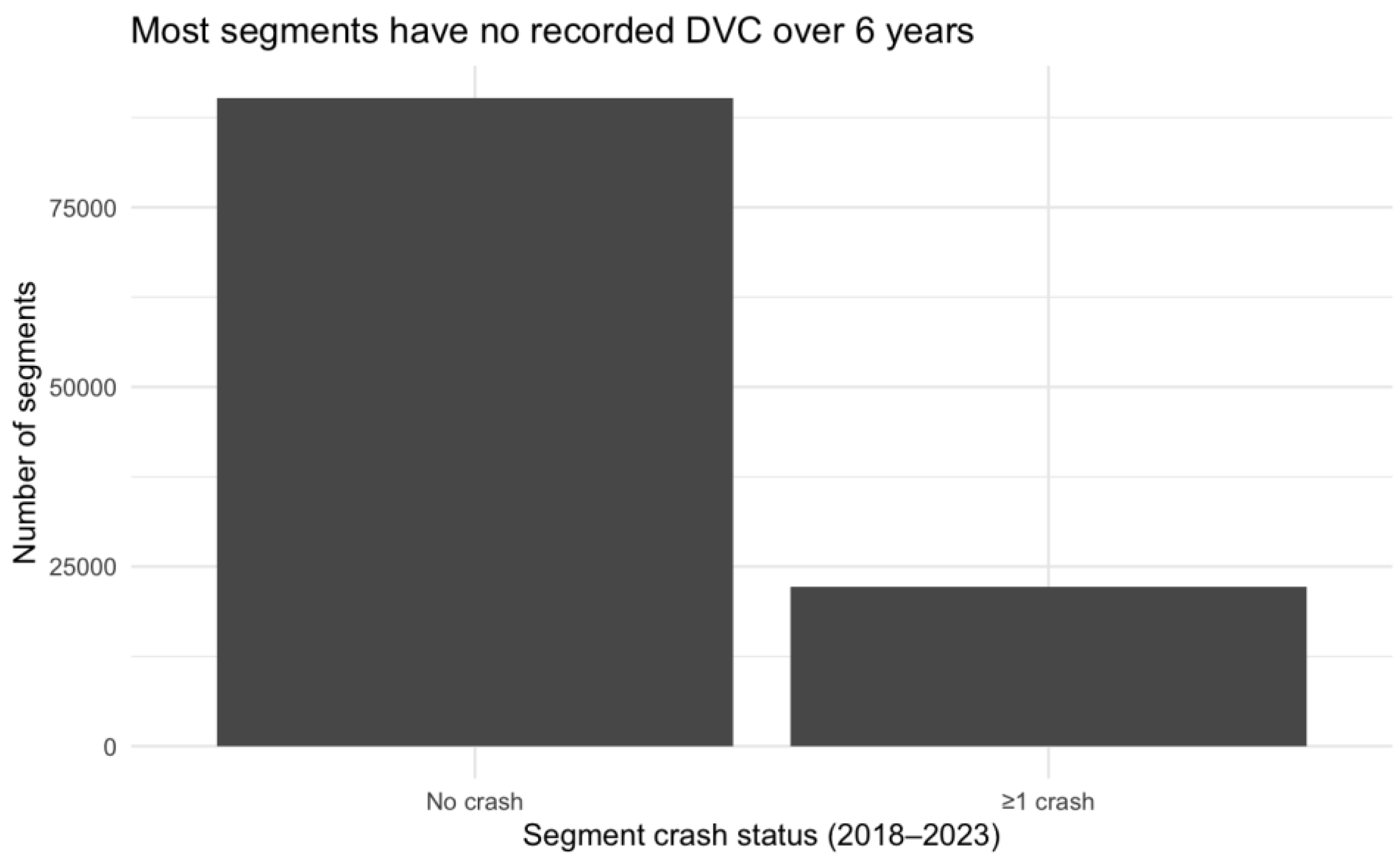
Figure 2.
Temporal dynamics of DVC occurrence probability.
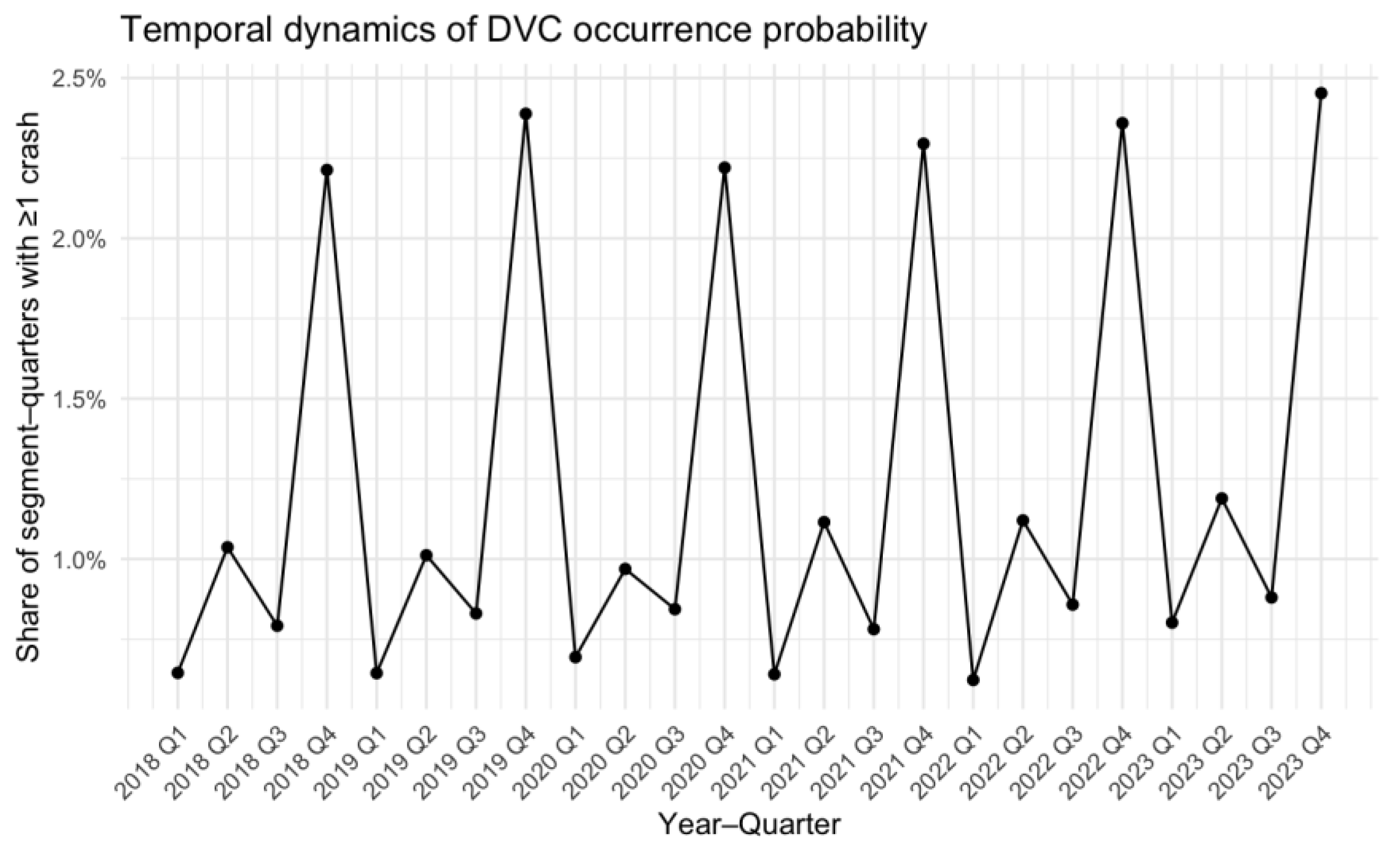
Figure 4.
Predicted Segment–Quarter Risk Classes for Q4 2024 in PA map.
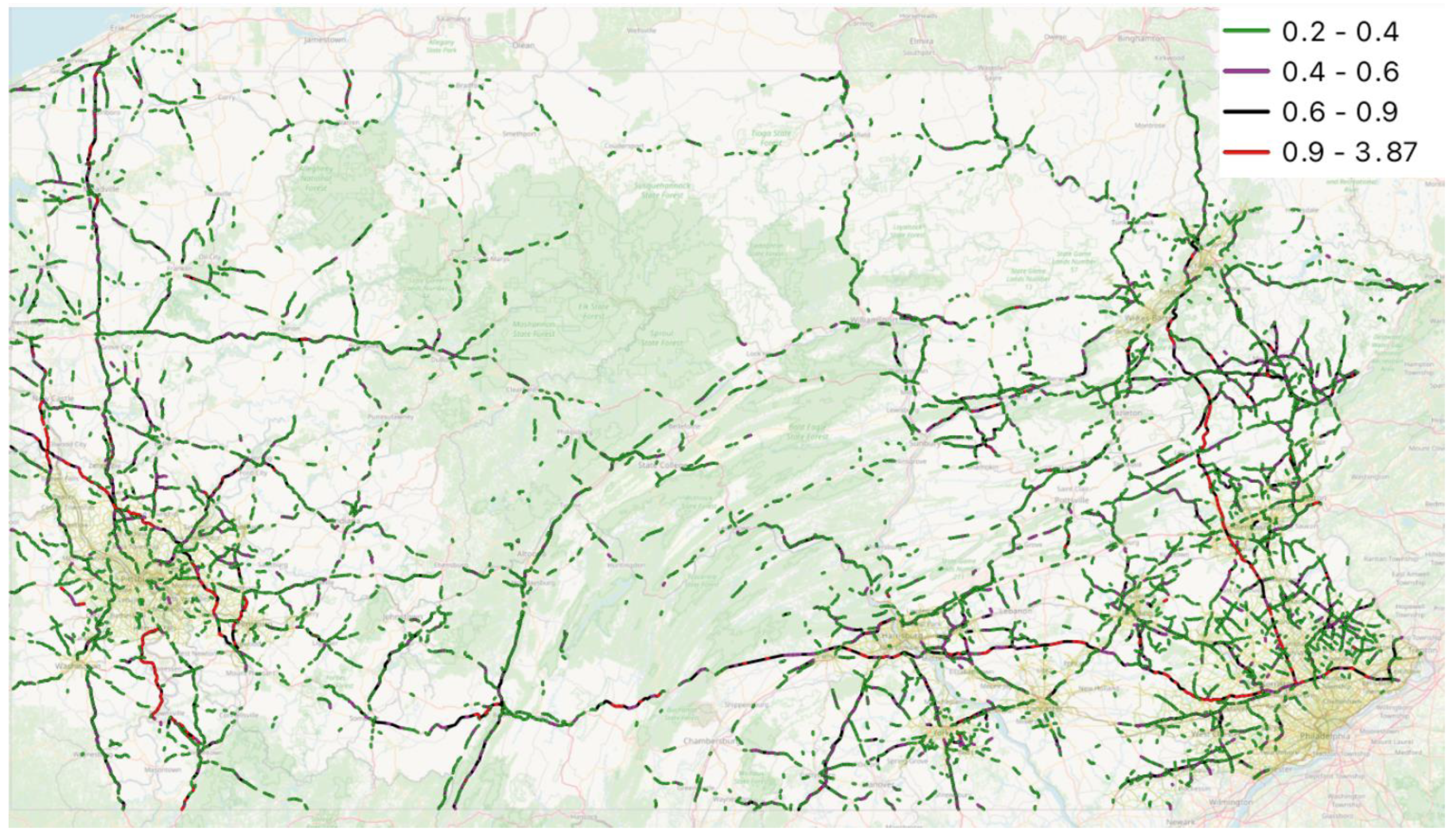
Figure 5.
Model Performance Across Segment–Quarter Risk Classes: Predicted and Observed DVC Counts for Q4 2024 in map between Harrisburg and Philadelphia.
Figure 5.
Model Performance Across Segment–Quarter Risk Classes: Predicted and Observed DVC Counts for Q4 2024 in map between Harrisburg and Philadelphia.
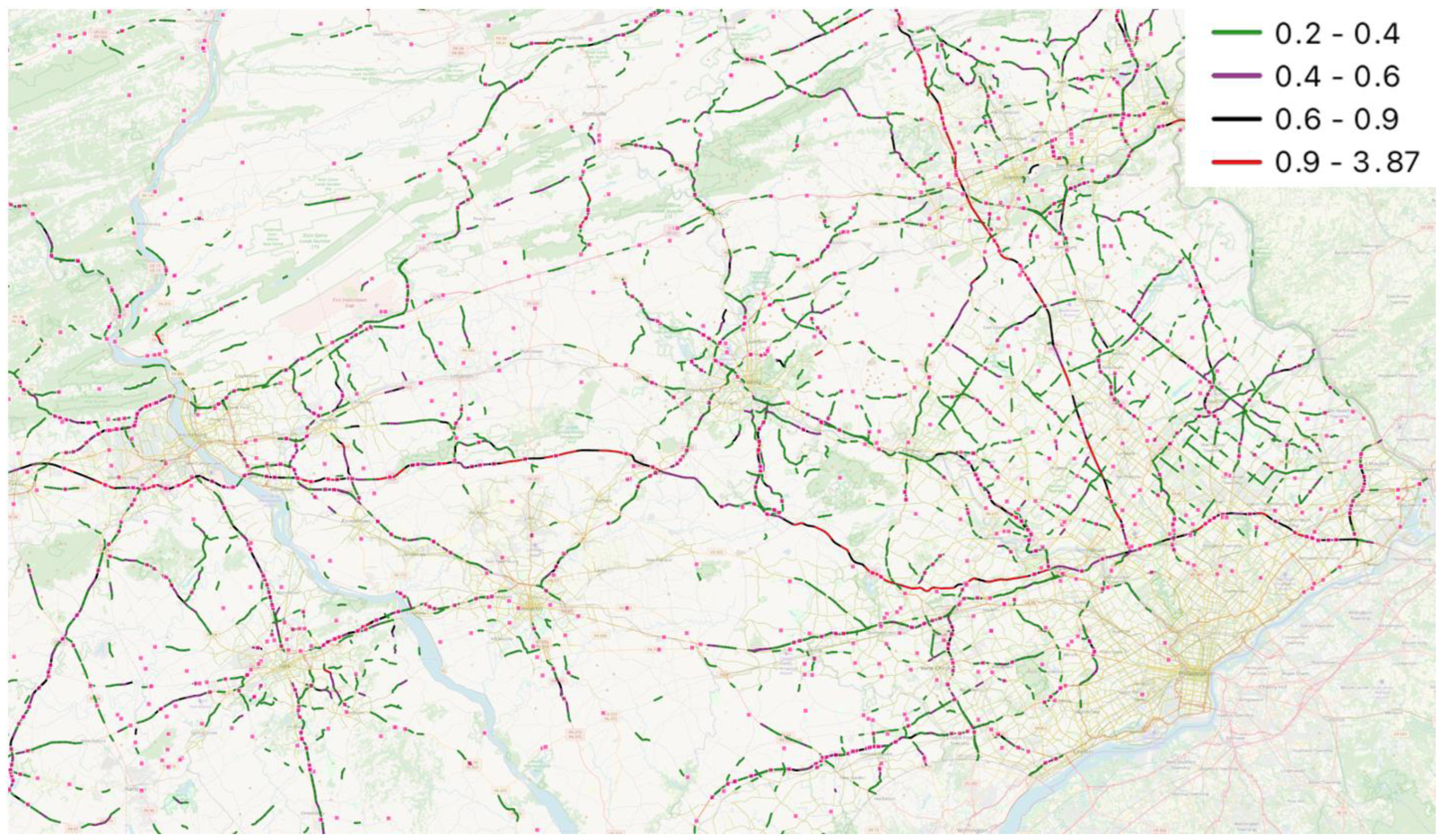

Table 1.
Posterior summaries for negative binomial models with and without quarter effects. Values are posterior means with 95% credible intervals in parentheses.
Table 1.
Posterior summaries for negative binomial models with and without quarter effects. Values are posterior means with 95% credible intervals in parentheses.
| Parameter | NB no Quarter | NB with Quarter effect |
|---|---|---|
| Fixed effect | ||
| Intercept | −12.95 (−13.26, −12.63) | –12.95 (–13.18, –12.73) |
| Total Width | −0.31 (−0.34, −0.27) | –0.32 (–0.35, –0.29) |
| Lane Count | 0.26 (0.23, 0.29) | 0.24 (0.22, 0.26) |
| Urban or Rural | −0.30 (−0.33, −0.27) | –0.30 (–0.33, –0.27) |
| Distribution | ||
| NB size (1/overdispersion) | 5.14 (3.69, 7.02) | 4.92 (3.55, 6.63) |
| Precision: QUARTER | — | 3.47 (1.41, 8.68) |
| Precision: seg_idx (BYM2) | 0.45 (0.43, 0.48) | 0.45 (0.43, 0.48) |
| Φ (seg_idx, BYM2 mixing) | 0.91 (0.90, 0.93) | 0.91 (0.90, 0.93) |
| Precision: TIME_KEY_Q (RW1) | 1.56 (1.02, 2.32) | 669.50 (307.78, 1463.09) |
| Model fit indices | ||
| DIC | 315,790.64 | 315 651.70 |
| WAIC | 315,494.47 | 315 422.49 |
| Effective number of parameters (pD) | 12,040.89 | 11 935.86 |
| Marginal log-likelihood | −203,788.20 | –203 746.27 |
Table 2.
Model Performance Across Segment–Quarter Risk Classes: Predicted and Observed DVC Counts for Q4 2024.
Table 2.
Model Performance Across Segment–Quarter Risk Classes: Predicted and Observed DVC Counts for Q4 2024.
| Risk class (crashes/segment–quarter) | Number of segments | Mean predicted count | Mean observed count | Proportion with ≥1 crash | Total observed crashes |
|---|---|---|---|---|---|
| 0–0.2 | 110,983 | 0.0250 | 0.0249 | 0.0237 | 2,767 |
| 0.2–0.4 | 1,178 | 0.262 | 0.257 | 0.223 | 303 |
| 0.4–0.6 | 154 | 0.485 | 0.558 | 0.442 | 86 |
| 0.6–0.9 | 46 | 0.695 | 0.435 | 0.304 | 20 |
| ≥0.9 | 16 | 1.09 | 1.12 | 0.75 | 18 |
Disclaimer/Publisher’s Note: The statements, opinions and data contained in all publications are solely those of the individual author(s) and contributor(s) and not of MDPI and/or the editor(s). MDPI and/or the editor(s) disclaim responsibility for any injury to people or property resulting from any ideas, methods, instructions or products referred to in the content. |
© 2025 by the authors. Licensee MDPI, Basel, Switzerland. This article is an open access article distributed under the terms and conditions of the Creative Commons Attribution (CC BY) license (http://creativecommons.org/licenses/by/4.0/).
Copyright: This open access article is published under a Creative Commons CC BY 4.0 license, which permit the free download, distribution, and reuse, provided that the author and preprint are cited in any reuse.


