Submitted:
01 December 2025
Posted:
03 December 2025
You are already at the latest version
Abstract
Reliable recognition of unmanned aerial vehicle (UAV) communication signals is important for low-altitude airspace safety and UAV monitoring systems. In real electromagnetic environments, UAV signals often show complex time-frequency patterns, and many unknown or new signal types can appear. These problems make open-set recognition necessary for practical UAV applications. In this paper, we propose a geometry-energy open-set recognition (GE-OSR) method designed for UAV signal monitoring. First, a time-frequency convolutional hybrid network is developed to learn multi-scale representations from raw UAV communication signals. Then, learnable class embeddings are added with a dual-constraint embedding loss to make the feature space more compact and separable. In addition, a free-energy alignment loss is introduced to guide the model to assign low energy to known UAV signals and high energy to unknown ones, which helps build an adaptive rejection boundary. Experiments under different SNRs and openness levels show that GE-OSR provides stable performance. At 0 dB SNR under high openness, the method improves OSCR by about 2.5% over the recent S3R model and more than 6% over other baselines. These results show that GE-OSR is effective for practical UAV signal identification and unknown signal detection in complex low-altitude environments.
Keywords:
unmanned aerial vehicles
; signal processing
; open-set recognition
; deep learning
; low-altitude security
1. Introduction
UAVs are now widely used across many fields, including smart agriculture [1], re-mote sensing [2], emergency response [3], logistics [4], and infrastructure inspection [5]. However, the rapid increase in low-altitude UAV operations has brought new challenges for airspace safety. Unauthorized or unknown drones can interfere with navigation and communication systems and even pose threats to critical infrastructure and national defense [6,7]. Therefore, reliable identification of UAV communication signals and detection of unknown or suspicious UAVs is essential for maintaining situational awareness in complex electromagnetic environments.
At present, UAV identification is mainly based on acoustic, visual, radar, and radio-frequency (RF) signals. Early works mainly relied on hand-crafted features and traditional machine learning models. For example, Muhammad et al. [8] used Mel-frequency cepstral coefficients from UAV sounds and trained support vector machines (SVMs) for recognition. Chu et al. [9] applied histograms of oriented gradients for visual detection, and Zhang et al. [10] used short-time Fourier transform and principal component analysis for radar-based classification. Nie et al. [11] combined fractal dimension and dual-spectrum features to extract RF fingerprints for UAV recognition. Although these methods can work in simple cases, their reliance on static, manual features makes it hard to adapt to noisy or changing environments.
Among all these data sources, RF signals are particularly valuable because they capture the communication behavior and operational status of UAVs. This makes them suitable for continuous monitoring and anti-UAV applications. In recent years, deep learning has greatly improved UAV signal recognition, since neural networks can learn hierarchical and discriminative features directly from raw IQ data. In other research fields, studies have explored many network designs [12,13,14,15] and learning strategies, such as few-shot [16,17], semi-supervised [18,19], self-supervised [20,21], and transfer learning [22,23], to improve model performance in difficult conditions. Inspired by these, Akter et al. [24] used convolutional neural networks (CNNs) with angle-of-arrival features for UAV recognition; Domenico et al. [25] proposed a real-time RF identification framework; and Cai et al. [26] built a lightweight multi-scale CNN for efficient UAV fingerprinting.
However, most existing works still assume a closed-set condition, in which all test classes are seen during training. In real UAV communication, this assumption is not true. New modulation types and private protocols often appear. Traditional Softmax-based models [27] must classify each input into a single known class and cannot recognize or reject new signals. To solve this problem, open-set recognition (OSR) has been proposed. OSR aims to build a model that not only classifies known samples correctly but also detects and rejects unknown samples.
Figure 1 shows the basic concept of OSR. In a closed-set scenario, the model performs well because all test samples come from known classes. However, when unknown samples appear, the closed-set model usually misclassifies them as one of the known classes. In contrast, an open-set model can not only correctly recognize known samples but also reject unknown ones. The concept of OSR was first introduced by Scheirer et al. [28]. Early studies used traditional classifiers like SVM [29], sparse representation [30], and k-nearest neighbors [31]. Later, Bendale et al. [32] proposed OpenMax, which brought OSR into the deep learning era. After that, researchers extended OSR by using counterfactual samples [33], generative adversarial networks [34,35], and reciprocal point learning [36,37]. Geng et al. [38] developed an OSR method based on a hierarchical Dirichlet process, and Wang et al. [39] employed energy modeling to construct high-energy regions for unknown detection.
Generally, OSR methods can be divided into two types: generative and discriminative. Generative methods try to create fake unknown samples, but it is hard to make them realistic. Discriminative methods aim to construct compact, separable feature spaces. However, they still face some problems, such as limited geometric diversity and sensitivity to noise or channel drift. Many of them use a single latent space, which makes it difficult to balance separability and stability. Also, fixed rejection thresholds reduce the ability to adapt to changing RF conditions. Although OSR has been applied to other fields such as bias detection [40] and pathogen identification [41], it is still rarely used for UAV RF signals. This task is difficult because UAVs often share similar frequency bands, have small differences between classes, and show strong non-stationary motion features, which make detecting unseen signals even harder.
To deal with these challenges, we propose the GE-OSR method for UAV signal classification. Unlike previous works, GE-OSR combines geometric embedding with energy-based modeling into a single framework. This design helps the model learn both the feature structure and the energy distribution, thereby achieving better recognition of known samples and stronger rejection of unknown ones. The main contributions of this paper are as follows:
- A time-frequency convolutional hybrid network for UAV signal representation. Considering the complex and variable patterns of UAV communication signals, a time-frequency convolutional hybrid network is introduced, combining time-frequency analysis with convolutional feature extraction, and ultimately providing more stable and representative signal features.
- A geometric embedding mechanism that enhances intra-class compactness and inter-class separability. For a clearer and more structured feature space, a geometric embedding mechanism is developed, incorporating learnable class embeddings and margin-aware constraints, which eventually lead to compact intra-class clusters and larger distances between classes.
- An energy-based regularization strategy for learning discriminative energy distributions. Faced with the difficulty of distinguishing known and unknown samples in open-set scenarios, an energy-based regularization strategy is adopted, consisting of an explicit energy formulation and its regularization term, and ultimately forming a more discriminative energy landscape.
- An adaptive energy threshold for open-set rejection. Instead of relying on a fixed threshold, an adaptive energy thresholding mechanism is introduced, using the empirical energy distribution of known classes, and finally achieving more reliable rejection of unknown signals under varying openness levels.
2. Materials and Methods
2.1. Feature Extractor
2.1.1. Time-Frequency Convolutional Hybrid Network
UAV RF signals are usually represented as in-phase and quadrature (IQ) sequences, which encode both temporal variations and spectral signatures. These signals evolve as they distribute energy across multiple frequency components, forming a complex pattern spanning two correlated domains. Conventional feature extractors often process them in isolation—either focusing on the time waveform or on its frequency spectrum. This separation makes it difficult for the model to learn how temporal and spectral cues interact. As a result, such approaches tend to miss critical cross-domain dependencies, limiting their capacity to capture the whole structure of UAV signal dynamics and to build strongly discriminative representations.
To overcome this limitation, we designed a time-frequency convolutional hybrid network. This structure leverages convolutional layers for local pattern modeling and Transformer self-attention for global dependency learning, enabling the network to build multi-scale representations that remain stable even under heavy noise. The overall architecture, shown in Figure 2, comprises two key modules: the time-frequency feature merging (TFFM) module and the convolutional-Transformer hybrid block (CTBlock).
2.1.2. Time-Frequency Feature Merging Module
The temporal and spectral components of UAV IQ signals differ substantially in scale, statistical distributions, and noise sensitivity. Simply concatenating them tends to create an imbalance between modalities and weakens the fusion effect. The proposed TFFM module addresses this by using a dual-branch structure that separately processes the time-domain and frequency-domain information, and then fuses them through a learnable attention mechanism.
As shown in Figure 3, the time branch applies a 1D convolution on the raw IQ sequence to capture short-term temporal features. The frequency branch first computes the fast Fourier transform (FFT) of the IQ signals and takes only the first half of the spectrum to avoid redundancy from the conjugate symmetry of real-valued signals. The spectral magnitudes are compressed using a logarithmic transformation to stabilize the dynamic range, and then passed through a 1D convolution to extract frequency features.
The outputs of the two branches have different lengths and are aligned by upsampling the frequency features to match the length of the time features. Each branch then passes through a 1 × 1 convolution with a residual connection to maintain feature consistency and channel compatibility. Finally, a lightweight convolution-based attention module computes time-wise fusion weights for the two branches. The attention weights are normalized with Softmax and applied to each branch to produce a fused representation. The final feature is a weighted combination of time and frequency features at each time step.
2.1.3. Convolutional-Transformer Hybrid Block
After fusing time and frequency information, the feature sequence still contains both local patterns and long-range dependencies. Convolutional layers are good at capturing local structures, while Transformer encoders are better at modeling global relationships. To leverage both, the CTBlock combines them in parallel, enabling the network to learn multi-scale features simultaneously.
As shown in Figure 4, the convolutional path uses large-kernel depthwise convolutions followed by pointwise projection to efficiently extract localized spatial-temporal features. Channel expansion is applied before pointwise projection to enrich local representations. In the Transformer path, the input sequence is first transposed and passed through Transformer encoder layers, where the self-attention mechanism captures long-range dependencies. The output is transposed back then. A learnable scalar gate with Sigmoid activation adaptively balances the contributions of the two paths. The fused output is finally added to the original input via a residual connection.
2.2. GE-OSR: An Open-Set Recognition Framework Based on Geometry-Energy Joint Modeling
2.2.1. Framework Overview
The GE-OSR framework is designed to utilize both the geometric relationships of feature vectors and their energy distributions. Its main goal is to correctly classify known UAV signal classes while rejecting unknown or unfamiliar signals. The overall architecture is shown in Figure 5.
As illustrated, GE-OSR contains four core components. First, a convolution-Transformer feature extractor fuses time and frequency information, generating multi-scale and discriminative representations of UAV signals. Second, a set of learnable class embeddings is introduced, which are optimized using a dual-constraint embedding loss (DCEL). This loss encourages intra-class compactness and enlarges inter-class separation, forming a feature space with clear geometric organization. Third, a free energy alignment loss (FEAL) shapes low-energy regions for known classes and high-energy regions for unknowns, providing a reliable energy-based boundary. Finally, during inference, an adaptive energy threshold is applied to distinguish unknown signals from known ones, enabling both closed-set classification and open-set rejection within a unified framework.
2.2.2. Feature Metrics and Class Embedding Initialization
The feature vectors produced by the extractor, denoted as , are normalized to unit length so that differences among samples are reflected only in their directions. Cosine similarity is adopted to measure the relationships between features and class embeddings, because it is bounded between -1 and 1 and provides a stable geometric interpretation when defining category boundaries. Given two feature vectors and , their cosine similarity is defined as:
In UAV signal feature space, class distributions are often uneven, and boundaries between nearby categories may become ambiguous, especially under noisy or overlapping conditions. To alleviate this, GE-OSR introduces a set of learnable class embeddings:
where represents the number of known classes, , and is the feature dimension of each sample . During initialization, every class embedding is sampled independently from a Gaussian distribution and then normalized onto the unit hypersphere:
This process distributes the embeddings roughly uniformly across the hypersphere, ensuring that they are nearly orthogonal to one another. Such spatial diversity serves as a substantial geometric prior, preventing early-stage collapse of class representations. As training progresses, these embeddings are treated as learnable parameters that gradually adapt through backpropagation, aligning with the empirical feature distributions of the known UAV signal classes.
2.2.3. Dual-Constraint Embedding Loss
To encourage both intra-class compactness and inter-class separability, the DCEL applies explicit geometric regularization in the embedding space. Let denote the feature vector of the -th sample, its label, and the embedding vector corresponding to class . The intra-class term encourages features to remain close to their corresponding class embeddings, thereby improving cohesion among samples of the same category. It is defined as:
where controls the sensitivity to deviation in similarity, and Delta specifies a soft-margin threshold between categories. By minimizing , the model continuously pulls features toward their corresponding embeddings, leading to dense and stable clusters within the representation space.
To avoid cluster overlap, the DCEL incorporates an inter-class separation term, which penalizes samples that appear excessively similar to incorrect class embeddings:
When a feature exhibits high similarity to an unrelated class embedding, rises sharply, forcing the network to expand the margins between classes.
The total loss is then defined as:
Together, these two terms create a structured embedding space in which features within the same category are tightly clustered, while features from different classes remain clearly separated.
2.2.4. Free Energy Alignment Loss
While shapes a discriminative feature geometry, it does not by itself provide a direct mechanism for identifying unknown inputs. To make this possible, we introduce the FEAL, inspired by the energy-based out-of-distribution detection work of Liu et al. [42], and adapt it to the geometry of our learned embeddings. The underlying idea is simple but effective: samples belonging to known categories should lie in low-energy regions. In contrast, those from unknown or unseen categories should lie in the high-energy areas. By explicitly minimizing the energy of known samples, the network learns to create compact low-energy basins in the representation space. Unlike earlier studies that convert Softmax logits into energy, we define energy directly through the cosine distance between a feature vector and the learnable class embeddings—thus maintaining consistency with the geometric modeling in the DCEL.
The cosine distance between two vectors and is defined as:
For a given feature , its distances to all class embeddings form the set:
and are mapped to the free energy as follows:
where is a temperature parameter controlling the smoothness of the energy landscape.
Intuitively, a feature vector close to a class embedding yields low energy, whereas one distant from all embeddings results in high energy. This property makes a natural criterion for distinguishing known from unknown signals.
To explicitly constrain known features toward the desired low-energy regions, the FEAL is defined as:
where is the target energy level and is the total number of samples. Minimizing encourages the free energy of known samples to converge around , forming compact, stable low-energy zones within the feature space.
Finally, the overall training objective combines the geometric and energy-based losses:
where and balance the contributions of the two terms. Joint optimization of DCEL and FEAL enables the model to construct a tightly clustered, energetically stable feature space.
2.2.5. Adaptive Energy Threshold Discrimination
In dynamic RF environments, the statistical distribution of signal features may shift during training or testing. A fixed energy threshold is therefore prone to bias and unstable classification. To address this issue, we design an adaptive energy thresholding strategy that updates the decision boundary online based on observed batch statistics. During each training iteration, the mean and variance of the free energy for known samples are calculated as:
where denotes the batch size and represents the free energy of the -th sample. Because these batch-level statistics are sensitive to noise and sampling fluctuations, we apply an exponential moving average (EMA) mechanism to stabilize them over time.
Given an update rate , the global mean and standard deviation at iteration are updated as:
This recursive formulation smooths short-term fluctuations while retaining the long-term statistical trend of the overall energy distribution. As a result, it provides a more stable and robust estimate of the global energy landscape, even under dynamic or noisy signal conditions.
Once the global statistics () are obtained, the rejection threshold is determined according to the Gaussian confidence interval principle:
where is a hyperparameter controlling the strictness of the boundary. A larger produces a more relaxed threshold, allowing greater tolerance to noise, whereas a smaller enforces stricter rejection, which is advantageous when unknown signals are more likely to appear.
During inference, the deep feature of each input sample is first extracted, and its free energy is computed. Classification is then performed based on the adaptive threshold :
If the signal originates from a known class, its energy remains below the threshold, and it is assigned to the class with the highest cosine similarity. Conversely, samples far from all class embeddings exhibit higher energy values and are rejected as unknown.
3. Results
3.1. Experimental Setup and Evaluation Protocol
3.1.1. Dataset Description
To evaluate the proposed open-set UAV signal recognition method, we used a self-developed lightweight target intelligent acquisition system to collect image transmission signals from DJI Phantom 4 RTK UAVs. The system covers a frequency range from 1.5 MHz to 8 GHz, has a real-time bandwidth over 30 MHz, and supports 32 simultaneous channels, allowing signals to be captured across multiple frequency bands. Experiments were conducted indoors to ensure signal stability. The receiving antenna was positioned approximately 20 meters from the UAV remote controller. The system’s center frequency was set to 5.8 GHz, and the 32 channels covered from 5.725 GHz to 5.850 GHz. Signals were continuously recorded for 10 seconds at 30 Msps (complex IQ). The data acquisition process is shown in Figure 6.
Ten UAVs of the same model but different individual units were used, each treated as a separate class. All UAVs transmitted signals independently without mutual interference. The UAV image transmission signals use OFDM modulation. To ensure each sample contains enough information and meets model input requirements, we extracted 10 ms segments from the recordings. Each segment was then downsampled to a fixed length of 4096 complex IQ points, followed by direct current removal and normalization. Spectrum and time-domain checks confirmed that signal bands and OFDM frames were intact.
After screening, 5,000 samples were collected (500 per UAV). Although the UAVs share the same protocol and hardware, small manufacturing differences introduce slight variations in RF signals, including oscillator drift, non-linear distortion, and front-end noise. These differences form unique RF fingerprints, which deep neural networks can learn for fine-grained UAV identification. This dataset serves as a benchmark for both closed-set classification and open-set UAV signal recognition.
3.1.2. Experimental Environment and Implementation Details
All experiments were done on a workstation with an Intel Core i9-11950H CPU and an NVIDIA RTX A3000 GPU. The model was implemented using PyTorch 2.2.2 with CUDA 12.1 support. To make the comparison fair, all models were trained and tested on the same dataset partition, using the same random seed. For the known classes, the data were divided into training, validation, and test sets in the ratio of 6:2:2. The detailed hyperparameter settings and implementation configurations are given in Table 1.
Each experiment was repeated several times, and we report the average results to reduce randomness and improve reproducibility.
3.1.3. Evaluation Metrics
To evaluate the model performance for both closed-set classification and open-set recognition, four main metrics were used: Acc, F1-score, AUROC, and OSCR.
Acc: Acc measures the overall proportion of correctly classified known samples and is defined as:
where , , , and denote true positives, true negatives, false positives, and false negatives, respectively. This metric provides an intuitive assessment of the closed-set classification precision.
F1-score: The F1-score provides a balanced measure between precision and recall, offering a fair assessment of classification performance, especially when the class distribution is uneven. It is computed as:
AUROC: AUROC quantifies how well the model distinguishes between known and unknown samples. It corresponds to the area under the receiver operating characteristic (ROC) curve, which captures the relationship between the true positive rate (TPR) and the false positive rate (FPR):
A higher AUROC value reflects a stronger ability to separate unknown samples from known ones, as well as a more stable decision boundary.
OSCR: OSCR jointly evaluates closed-set classification accuracy and open-set rejection performance, providing a unified view of recognition effectiveness. It is defined as:
where and denote the number of closed-set and open-set samples, respectively; represents the model’s confidence score, and is the decision threshold. Higher OSCR values indicate a better overall trade-off between correctly classifying known classes and successfully rejecting unknown ones.
3.2. Closed-Set Recognition Performance
A strong closed-set classification backbone is the prerequisite for reliable open-set recognition. To assess the effectiveness of the proposed feature extractor in terms of ac-curacy, noise robustness, and parameter efficiency, we compared it with several representative IQ-based electromagnetic signal classification models, including ResNet [43], GRU [44], MCLDNN [45], and IQformer [46].
Figure 7 shows the closed-set recognition accuracy of all models across different SNRs. As expected, performance improves as SNR increases. However, the differences between models become pronounced at low SNR (SNR < 0 dB). Under substantial noise interference, both GRU and IQformer show a noticeable drop in accuracy, while ResNet and MCLDNN remain relatively stable but still underperform the proposed model. Across the entire SNR range, our method maintains the highest accuracy, suggesting stronger resilience and better generalization in noisy communication environments.
At an SNR of 0 dB, the detailed results are listed in Table 2.
The proposed model achieves the highest Acc and F1-score among all compared methods, while also maintaining the lowest parameter count (0.062M). This balance indicates that the network can efficiently learn discriminative representations of UAV signals with minimal computational cost—an essential advantage for real-time or embedded anti-UAV systems.
To better understand category-level performance, Figure 8 presents the confusion matrices of all models at 0 dB SNR. The proposed model shows strong diagonal dominance, indicating that most samples are correctly classified. Misclassifications are fewer and less severe compared with the baseline models, consistent with the quantitative results.
To provide a feature-level view, Figure 9 visualizes the learned representations using t-SNE. The proposed model produces compact and well-separated clusters, with samples from the same class grouped tightly and clear margins between classes. In contrast, features from the baseline models show noticeable overlap, indicating weaker inter-class separation. This visualization supports the observed quantitative improvements.
In summary, these results show that the proposed model achieves strong closed-set classification. The learned feature space demonstrates compact intra-class clusters and clear inter-class boundaries, which improves accuracy under noisy conditions and provides a solid basis for the subsequent geometry-energy-based open-set recognition.
3.3. Open-Set Recognition Results
To comprehensively evaluate the effectiveness of the proposed GE-OSR framework in open-set recognition tasks, the performance was compared with several baseline methods, including OpenMax [32], ARPL [37], PROSER [47], CSSR [48], and the state-of-the-art S3R [49]. Experiments were conducted along two dimensions: (1) varying levels of openness, and (2) different SNR conditions.
First, the number of known classes was fixed at four, and the SNR was set to 0 dB to examine how the number of unknown classes affects recognition performance. Table 3 presents the AUROC results for each method under different numbers of unknown classes. As the number of unknown classes increases, AUROC values decrease consistently across all methods, reflecting the growing difficulty of open-set recognition at higher openness levels. Among all methods, GE-OSR achieves the highest AUROC scores and exhibits the smallest decline as openness increases. For instance, with six unknown classes, GE-OSR still reaches an AUROC of 96.39% ± 0.56%, demonstrating strong performance even under challenging conditions. The relatively high average AUROC and small standard deviations indicate that GE-OSR is stable and reliable across different openness settings.
Table 4 shows the OSCR results under the same experimental setup. Similar to AUROC, OSCR decreases gradually as the number of unknown classes grows. However, GE-OSR consistently outperforms other methods in terms of OSCR, maintaining high scores across all openness levels. For example, when six unknown classes are present, GE-OSR achieves an OSCR of 95.39% ± 0.67%, which is higher than all baseline methods.
In the subsequent experiments, the number of known categories was fixed at four and the number of unknown categories at six. Since open-set UAV signal recognition needs to consider both classifying known categories correctly and rejecting unknown ones, OSCR is a more suitable metric as it evaluates both at the same time. Therefore, Figure 10 illustrates the OSCR performance of each method under different SNR conditions, providing a clearer view of how noise affects the open-set classification ability.
As shown in Figure 10, the OSCR performance of all models improves with increasing SNR. At low SNR, the proposed GE-OSR model clearly outperforms the other methods. When the SNR is moderate or high (≥ 0 dB), S3R also performs well, but GE-OSR still achieves higher performance, reaching an OSCR of about 0.96 at high SNR. This means the model has a higher upper limit of performance and is more stable.
To show how different methods separate features, Figure 11 gives t-SNE visualizations for known and unknown classes.
As shown in Figure 11, the features learned by the proposed GE-OSR framework display the most compact intra-class clusters and the clearest inter-class separations. More importantly, unknown samples are well-isolated from known clusters, forming distinct and independent regions in the feature space.
3.4. Impact of Threshold Settings on Open-Set Recognition Performance
Threshold selection is very important in open-set recognition because it affects both the classification accuracy of known categories and the rejection rate of unknown signals. To show how this balance works, Figure 12a presents the free-energy distributions for known and unknown samples. Figure 12b shows how recognition accuracy changes as the rejection threshold varies. These figures help illustrate how the adaptive threshold affects the decision boundary and maintains stable recognition.
As seen in Figure 12a, most of the known samples are located in the low-energy region, while the unknown samples are mainly in the higher-energy region. This shows that there is a clear separation between the known and unknown signals in the energy space. However, some known samples still have relatively high energy. This usually happens when the signal has low SNR, channel distortion, or is close to the class boundary, which makes its features deviate from the class embedding. The dashed line represents the adaptive threshold , which is approximately in the valley between the two distributions. This threshold can automatically adjust based on the energy distribution, so it does not need to be set manually and still effectively separates known and unknown samples.
Figure 12b shows how the threshold value affects the model’s performance. At the current threshold, the GE-OSR model achieves 92.50% accuracy on known UAV signals and rejects 98.67% of unknown ones. These results show that the proposed method can achieve a good balance between correctly recognizing known classes and rejecting unfamiliar signals. The open-set confusion matrix is shown in Figure 13.
From Figure 13, it can be seen that the proposed model maintains high classification accuracy across all known UAV categories and rejects about 98% of un-known samples. Most of the known classes are clearly separated, but there is still some confusion between UAV2 and the Unknown class. About 28% of UAV2 samples are wrongly rejected as unknown, and about 1% of unknown signals are predicted as UAV2. This kind of mistake may be caused by the high similarity between the feature distributions of UAV2 and some unseen signal types, leading to partial overlap in the embedding space.
Even with this problem, the adaptive energy-thresholding method can still work effectively. It can automatically adjust the decision boundary as the feature distribution changes, ensuring the model’s recognition and rejection abilities remain stable across different noise levels and openness conditions.
3.5. Ablation Studies
To study how each part of the GE-OSR model contributes to the final performance, we did several ablation experiments. Three modules were tested: TFFM, DCEL, and FEAL. These modules were added one by one to observe their individual influence on AUROC and OSCR.
All experiments were conducted under the same conditions and repeated 5 times to improve reliability. The mean and standard deviation of the performance are shown in Table 5. For the version without TFFM, we used a 1 × 1 convolutional layer to maintain the same feature dimension, and all other settings remained unchanged.
From Table 5, we can see that the basic model achieves AUROC of 70.09% and OSCR of 62.35%. After adding TFFM, both indexes increase significantly, by +14.5% in AUROC and +19.7% in OSCR. This shows that time–frequency fusion can extract more useful in-formation and make the model more robust to noise. After adding DCEL, the two indicators increase again (+4.9% AUROC, +6.8% OSCR), indicating that the geometric constraint can bring intra-class features closer and enlarge the inter-class margin. When FEAL is also used, both metrics improve by around 6-7%, indicating that controlling the energy distribution is important for a smoother open-set boundary.
In conclusion, TFFM provides a solid foundation for feature extraction, DCEL helps build better geometric representations across classes, and FEAL clarifies the energy distribution between known and unknown areas. When all three modules are combined, the GE-OSR model demonstrates strong discriminative ability and stable recognition performance across different open-set UAV signal environments.
4. Discussion
The mechanism of GE-OSR has two main parts. The DCEL module improves the compactness of feature distribution by pulling samples of the same class closer to their embeddings, so features from the same UAV become more clustered in the embedding space. At the same time, the FEAL module keeps the energy of known samples within a stable, low range, while unknown samples are pushed to higher-energy areas. When these two parts work together, they can build a clear, stable boundary in the geometry-energy space, which helps the model distinguish between known and unseen UAV signal classes more accurately and robustly.
The multi-scale time-frequency modeling in TFFM and CTBlock helps the network extract features that are both more discriminative and more resistant to noise. As a result, the model can still perform well even under strong noise. At the same time, the model has only about 0.062 million parameters, making it very lightweight and suitable for real-time UAV detection systems, including portable or edge devices often used in smart cities, emergency response, and perimeter surveillance.
However, there are still some limitations. The EMA-based threshold can sometimes be slow to react when channel conditions change quickly. The model may also fail to identify signals that are completely different from all known categories. In addition, the delay still needs to be reduced to improve the system’s performance in real-time tasks. In the future, we plan to improve the threshold method, enhance generalization to unseen signals, and further simplify the model architecture to meet the strict real-time and operational requirements of practical UAV monitoring applications.
Overall, GE-OSR demonstrates high accuracy, clear interpretability, and strong generalization ability. The model maintains very stable performance in open-set recognition, handling low signal-to-noise ratios and a large number of unknown signals with ease, whereas most existing methods often fail under such conditions. These results indicate that the joint constraint of geometry and energy is an effective strategy for managing complex electromagnetic signal environments. The combination of geometry and energy not only supports robust UAV signal recognition but also provides a promising approach for other intelligent perception tasks in open and dynamic environments, such as anti-drone surveillance, autonomous UAV navigation, and urban airspace management.
5. Conclusions
This paper proposes GE-OSR, a UAV signal recognition model that integrates geometric structure and energy control. By combining feature geometry with energy adjustment, GE-OSR achieves more stable and robust decisions, outperforming existing methods by up to 2.5% OSCR under challenging conditions. The model is not only accurate but also lightweight and interpretable, making it suitable for real-time deployment in UAV monitoring and anti-drone systems. The geometry-energy modeling approach introduced here offers a promising direction for future intelligent sensing systems. In particular, its ability to distinguish known and unknown UAV signals in complex electromagnetic environments is directly relevant to low-altitude airspace safety, smart city UAV management, and autonomous drone operations.
6. Patents
This work has resulted in the following patent:
Zhou, F.; Long, Y.; Zhou, H.; Ren, H.; Gao, R.; Li, H.; Yi, Z.; Hu, J.; Wang, W. An Open-Set UAV Signal Recognition Method Based on Class Center Learning. China National Intellectual Property Administration (CNIPA), Application No. CN202510455917.9, Publication No. CN120408403A, Filed on April 11, 2025, Published on August 1, 2025.
Supplementary Materials
No supplementary materials are available.
Author Contributions
Conceptualization, Y.L. and H.Z.; data curation, Y.L. and H.Z.; formal analysis, W.Y. and H.R.; Funding acquisition, H.Z.; investigation, Y.L.; methodology, Y.L.; project administration, W.Y; resources, H.Z.; supervision, H.Z. and F.Z.; validation, Y.L., W.Y. and H.R.; visualization, Y.L.; writing—original draft preparation, Y.L.; writing—review and editing, H.Z., W.Y, H.R., F.Z. and Y.Z. All authors have read and agreed to the published version of the manuscript.
Funding
This research was funded by National Natural Science Foundation of China, grant number 62231027 and 62471385.
Data Availability Statement
The data presented in this study are available on request from the corresponding author due to confidentiality and security restrictions.
Acknowledgments
The authors would like to acknowledge the 36th Research Institute of China Electronics Technology Group Corporation (CETC36) for their support in providing the experimental facilities and equipment for this research.
Conflicts of Interest
The authors declare no conflicts of interest.:
Abbreviations
The following abbreviations are used in this manuscript:
| Acc | Accuracy |
| AUROC | Area under the receiver operating characteristic curve |
| CTBlock | Convolutional-Transformer hybrid block |
| DCEL | Dual-constraint embedding loss |
| FEAL | Free energy alignment loss |
| GE-OSR | Geometry-energy open-set recognition |
| IQ | In-phase and quadrature |
| OSCR | Open-set classification rate |
| OSR | Open-set recognition |
| RF | Radio frequency |
| SNR | Signal-to-noise ratio |
| TFFM | Time-frequency feature merging |
| UAV | Unmanned aerial vehicle |
References
- Maddikunta, P.K.R.; Hakak, S.; Alazab, M.; Bhattacharya, S.; Gadekallu, T.R.; Khan, W.Z. Unmanned Aerial Vehicles in Smart Agriculture: Applications, Requirements, and Challenges. IEEE Sens. J. 2021, 21, 17608–17619. [Google Scholar] [CrossRef]
- Dong, H.; Dong, J.; Sun, S.; Bai, T.; Zhao, D.; Yin, Y.; Shen, X.; Wang, Y.; Zhang, Z.; Wang, Y. Crop Water Stress Detection Based on UAV Remote Sensing Systems. Agric. Water Manag. 2024, 303, 109059. [Google Scholar] [CrossRef]
- Surman, K.; Lockey, D. Unmanned Aerial Vehicles and Pre-Hospital Emergency Medicine. Scand. J. Trauma Resusc. Emerg. Med. 2024, 32, 9. [Google Scholar] [CrossRef] [PubMed]
- Saunders, J.; Saeedi, S.; Li, W. Autonomous Aerial Robotics for Package Delivery: A Technical Review. J. Field Robot. 2024, 41, 3–49. [Google Scholar] [CrossRef]
- Duan, Q.; Chen, B.; Luo, L. Rapid and Automatic UAV Detection of River Embankment Piping. Water Resour. Res. 2025, 61, e2024WR038931. [Google Scholar] [CrossRef]
- Tlili, F.; Ayed, S.; Fourati, L.C. Advancing UAV Security with Artificial Intelligence: A Comprehensive Survey of Techniques and Future Directions. Internet Things 2024, 27, 101281. [Google Scholar] [CrossRef]
- Medaiyese, O.O.; Ezuma, M.; Lauf, A.P.; Guvenc, I. Wavelet Transform Analytics for RF-Based UAV Detection and Identification System Using Machine Learning. Pervasive Mob. Comput. 2022, 82, 101569. [Google Scholar] [CrossRef]
- Anwar, M.Z.; Kaleem, Z.; Jamalipour, A. Machine Learning Inspired Sound-Based Amateur Drone Detection for Public Safety Applications. IEEE Trans. Veh. Technol. 2019, 68, 2526–2534. [Google Scholar] [CrossRef]
- Chu, H.; Zhang, D.; Shao, Y.; Chang, Z.; Guo, Y.; Zhang, N. Using HOG Descriptors and UAV for Crop Pest Monitoring. In Proceedings of the Chinese Automation Congress (CAC), Xi’an, China, 30 November-2 December 2018; 2018; pp. 1516–1519. [Google Scholar]
- Zhang, P.; Yang, L.; Chen, G.; Li, G. Classification of Drones Based on Micro-Doppler Signatures with Dual-Band Radar Sensors. In Proceedings of the Progress in Electromagnetics Research Symposium - Fall (PIERS - FALL), Singapore, 19-22 November 2017; 2017; pp. 638–643. [Google Scholar]
- Nie, W.; Han, Z.; Zhou, M.; Xie, L.; Jiang, Q. UAV Detection and Identification Based on WiFi Signal and RF Fingerprint. IEEE Sens. J. 2021, 21, 13540–13550. [Google Scholar] [CrossRef]
- Wang, X. Electronic Radar Signal Recognition Based on Wavelet Transform and Convolution Neural Network. Alex. Eng. J. 2022, 61, 3559–3569. [Google Scholar] [CrossRef]
- Gu, Z.; Ma, Q.; Gao, X.; You, J.; Cui, T. Direct Electromagnetic Information Processing with Planar Diffractive Neural Network. Sci. Adv. 2024, 10, eado3937. [Google Scholar] [CrossRef] [PubMed]
- Chu, T.; Zhou, H.; Ren, Z.; Ye, Y.; Wang, C.; Zhou, F. Intelligent Detection of Low-Slow-Small Targets Based on Passive Radar. Remote Sens. 2025, 17, 961. [Google Scholar] [CrossRef]
- Cucchi, M.; Gruener, C.; Petrauskas, L.; Steiner, P.; Tseng, H.; Fischer, A.; Penkovsky, B.; Matthus, C.; Birkholz, P.; Kleemann, H.; Leo, K. Reservoir Computing with Biocompatible Organic Electrochemical Networks for Brain-Inspired Biosignal Classification. Sci. Adv. 2021, 7, eabh0693. [Google Scholar] [CrossRef] [PubMed]
- Zhou, H.; Bai, J.; Wang, Y.; Jiao, L.; Zheng, S.; Shen, W.; Xu, J.; Yang, X. Few-Shot Electromagnetic Signal Classification: A Data Union Augmentation Method. Chin. J. Aeronaut. 2022, 35, 49–57. [Google Scholar] [CrossRef]
- Sun, Z.; Wang, Z.; Wang, M. SLTRN: Sample-Level Transformer-Based Relation Network for Few-Shot Classification. Neural Netw. 2024, 176, 106344. [Google Scholar] [CrossRef]
- Liu, Z.; Pei, W.; Lan, D.; Ma, Q. Diffusion Language-Shapelets for Semi-Supervised Time-Series Classification. In Proceedings of the AAAI Conference on Artificial Intelligence, Vancouver, Canada, 20-27 February 2024; 2024; pp. 14079–14087. [Google Scholar]
- Zhou, H.; Jiao, L.; Zheng, S.; Yang, L.; Shen, W.; Yang, X. Generative Adversarial Network-Based Electromagnetic Signal Classification: A Semi-Supervised Learning Framework. China Commun. 2020, 17, 157–169. [Google Scholar] [CrossRef]
- Liu, J.; Chen, S. TimesURL: Self-Supervised Contrastive Learning for Universal Time Series Representation Learning. In Proceedings of the AAAI Conference on Artificial Intelligence, Vancouver, Canada, 20-27 February 2024; 2024; pp. 13918–13926. [Google Scholar]
- Hou, K.; Du, X.; Cui, G.; Chen, X.; Zheng, J.; Rong, Y. A Hybrid Network-Based Contrastive Self-Supervised Learning Method for Radar Signal Modulation Recognition. IEEE Trans. Veh. Technol. 2025, 1–15. [Google Scholar] [CrossRef]
- Zhou, H.; Wang, X.; Bai, J.; Xiao, Z. Modulation Signal Recognition Based on Selective Knowledge Transfer. In Proceedings of the GLOBECOM 2022 - 2022 IEEE Global Communications Conference, Rio de Janeiro, Brazil, 04-08 December 2022; 2022; pp. 1875–1880. [Google Scholar]
- Wang, M.; Lin, Y.; Tian, Q.; Si, G. Transfer Learning Promotes 6G Wireless Communications: Recent Advances and Future Challenges. IEEE Trans. Reliab. 2021, 70, 790–807. [Google Scholar] [CrossRef]
- Akter, R.; Doan, V.; Thien, H.; Kim, D. RFDOA-Net: An Efficient ConvNet for RF-Based DOA Estimation in UAV Surveillance Systems. IEEE Trans. Veh. Technol. 2021, 70, 12209–12214. [Google Scholar] [CrossRef]
- Lofù, D.; Gennaro, P.D.; Tedeschi, P.; Noia, T.D.; Sciascio, E.D. URANUS: Radio Frequency Tracking, Classification and Identification of Unmanned Aircraft Vehicles. IEEE Open J. Veh. Technol. 2023, 4, 921–935. [Google Scholar] [CrossRef]
- Cai, Z.; Wang, Y.; Jiang, Q.; Gui, G.; Sha, J. Toward Intelligent Lightweight and Efficient UAV Identification with RF Fingerprinting. IEEE Internet Things J. 2024, 11, 26329–26339. [Google Scholar] [CrossRef]
- Zhang, H.; Zhou, H.; Wang, L.; Zhou, F. Spatial Distribution Feature Extraction Network for Open Set Recognition of Electromagnetic Signal. Comput. Model. Eng. Sci. 2024, 139, 279–296. [Google Scholar] [CrossRef]
- Scheirer, W.J.; Rocha, A.d.R.; Sapkota, A.; Boult, T.E. Toward Open Set Recognition. IEEE Trans. Pattern Anal. Mach. Intell. 2013, 35, 1757–1772. [Google Scholar] [CrossRef] [PubMed]
- Scheirer, W.J.; Jain, L.P.; Boult, T.E. Probability Models for Open Set Recognition. IEEE Trans. Pattern Anal. Mach. Intell. 2014, 36, 2317–2324. [Google Scholar] [CrossRef]
- Zhang, H.; Patel, V.M. Sparse Representation-Based Open Set Recognition. IEEE Trans. Pattern Anal. Mach. Intell. 2017, 39, 1690–1696. [Google Scholar] [CrossRef]
- Júnior, P.R.M.; de Souza, R.M.; Werneck, R.d.O.; Oliveira, L.S.; Papa, J.P. Nearest Neighbors Distance Ratio Open-Set Classifier. Mach. Learn. 2017, 106, 359–386. [Google Scholar] [CrossRef]
- Bendale, A.; Boult, T.E. Towards Open Set Deep Networks. In Proceedings of the 2016 IEEE Conference on Computer Vision and Pattern Recognition (CVPR), Las Vegas, NV, USA, 27-30 June 2016; 2016; pp. 1563–1572. [Google Scholar]
- Neal, L.; Olson, M.; Fern, X.; Wong, W.; Li, F. Open Set Learning with Counterfactual Images. In Proceedings of the European Conference on Computer Vision (ECCV), Munich, Germany, 8-14 September 2018; 2018; pp. 620–635. [Google Scholar]
- Yang, Y.; Hou, C.; Lang, Y.; Guan, D.; Huang, D.; Xu, J. Open-Set Human Activity Recognition Based on Micro-Doppler Signatures. Pattern Recognit. 2019, 85, 60–69. [Google Scholar] [CrossRef]
- Oza, P.; Patel, V.M. C2AE: Class Conditioned Auto-Encoder for Open-Set Recognition. In Proceedings of the IEEE/CVF Conference on Computer Vision and Pattern Recognition (CVPR), Long Beach, CA, USA, 15-20 June 2019; 2019; pp. 2302–2311. [Google Scholar]
- Chen, G.; Zhang, Y.; Liang, X.; Liu, Y.; Lin, L. Learning Open Set Network with Discriminative Reciprocal Points. In Proceedings of the European Conference on Computer Vision (ECCV), Glasgow, UK, 23-28 August 2020; 2020; pp. 507–522. [Google Scholar]
- Chen, G.; Peng, P.; Wang, X.; Tian, Y. Adversarial Reciprocal Points Learning for Open Set Recognition. IEEE Trans. Pattern Anal. Mach. Intell. 2022, 44, 8065–8081. [Google Scholar] [CrossRef]
- Geng, C.; Chen, S. Collective Decision for Open Set Recognition. IEEE Trans. Knowl. Data Eng. 2022, 34, 192–204. [Google Scholar] [CrossRef]
- Wang, H.; Pang, G.; Wang, P.; Zhang, L.; Wei, W.; Zhang, Y. Glocal Energy-Based Learning for Few-Shot Open-Set Recognition. In Proceedings of the IEEE/CVF Conference on Computer Vision and Pattern Recognition (CVPR), Vancouver, BC, Canada, 18-22 June 2023; 2023; pp. 7507–7516. [Google Scholar]
- D’Incà, M.; Peruzzo, E.; Mancini, M.; Xu, D.; Goel, V.; Xu, X.; Wang, Z.; Shi, H.; Sebe, N. OpenBias: Open-set Bias Detection in Text-to-Image Generative Models. In Proceedings of the IEEE/CVF Conference on Computer Vision and Pattern Recognition (CVPR), Seattle, WA, USA, 17-21 June 2024; 2024; pp. 12225–12235. [Google Scholar]
- Zhu, L.; Yang, Y.; Xu, F.; Lu, X.; Shuai, M.; An, Z.; Chen, X.; Li, H.; Martin, F.L.; Vikesland, P.J.; Ren, B.; Tian, Z.; Zhu, Y.; Cui, L. Open-Set Deep Learning-Enabled Single-Cell Raman Spectroscopy for Rapid Identification of Airborne Pathogens in Real-World Environments. Sci. Adv. 2025, 11, eadp7991. [Google Scholar] [CrossRef]
- Liu, W.; Wang, X.; Owens, J.D.; Li, Y. Energy-based out-of-distribution detection. In Proceedings of the 34th International Conference on Neural Information Processing Systems (NeurIPS 2020), Vancouver, BC, Canada, 6-12 December 2020; 2020. [Google Scholar]
- He, K.; Zhang, X.; Ren, S.; Sun, J. Deep Residual Learning for Image Recognition. In Proceedings of the IEEE Conference on Computer Vision and Pattern Recognition (CVPR), Las Vegas, NV, USA, 27-30 June 2016; 2016; pp. 770–778. [Google Scholar]
- Chung, J.; Gulcehre, C.; Cho, K.H.; Bengio, Y. Empirical Evaluation of Gated Recurrent Neural Networks on Sequence Modeling. arXiv 2014, arXiv:1412.3555. [Google Scholar] [CrossRef]
- Xu, J.; Luo, C.; Parr, G.; Luo, Y. A Spatiotemporal Multi-Channel Learning Framework for Automatic Modulation Recognition. IEEE Wirel. Commun. Lett. 2020, 9, 1629–1632. [Google Scholar] [CrossRef]
- Shao, M.; Li, D.; Hong, S.; Qi, J.; Sun, H. IQFormer: A Novel Transformer-Based Model with Multi-Modality Fusion for Automatic Modulation Recognition. IEEE Trans. Cogn. Commun. Netw. 2025, 11, 1623–1634. [Google Scholar] [CrossRef]
- Zhou, D.; Ye, H.; Zhan, D. Learning Placeholders for Open-Set Recognition. In Proceedings of the IEEE/CVF Conference on Computer Vision and Pattern Recognition (CVPR), Nashville, TN, USA, 20-25 June 2021; 2021; pp. 4399–4408. [Google Scholar]
- Huang, H.; Wang, Y.; Hu, Q.; Cheng, M. Class-Specific Semantic Reconstruction for Open Set Recognition. IEEE Trans. Pattern Anal. Mach. Intell. 2023, 45, 4214–4228. [Google Scholar] [CrossRef]
- Yu, N.; Wu, J.; Zhou, C.; Shi, Z.; Chen, J. Open Set Learning for RF-Based Drone Recognition via Signal Semantics. IEEE Trans. Inf. Forensics Security 2024, 19, 9894–9909. [Google Scholar] [CrossRef]
Figure 1.
Conceptual illustration of open-set recognition: (a) Closed-set recognition: all test samples belong to known classes; (b) Closed-set classifier encountering unknown samples: unknown data are incorrectly assigned to the nearest known class; (c) Open-set recognition: known samples are correctly classified while unknown ones are rejected.
Figure 2.
Architecture of the proposed time-frequency feature extraction network.
Figure 3.
Structure of the time-frequency feature merging module.
Figure 4.
Structure of the convolutional-Transformer hybrid block.
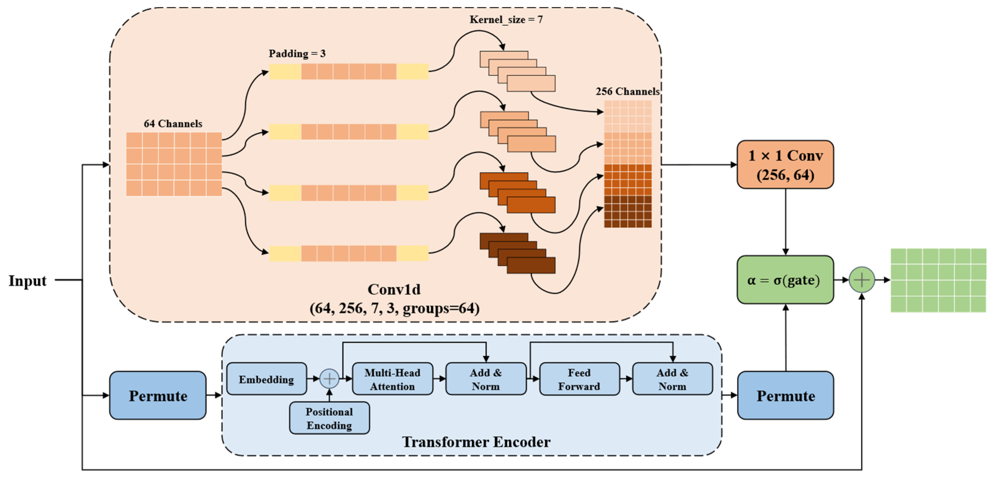
Figure 5.
Overall architecture of the geometry-energy open-set recognition framework.
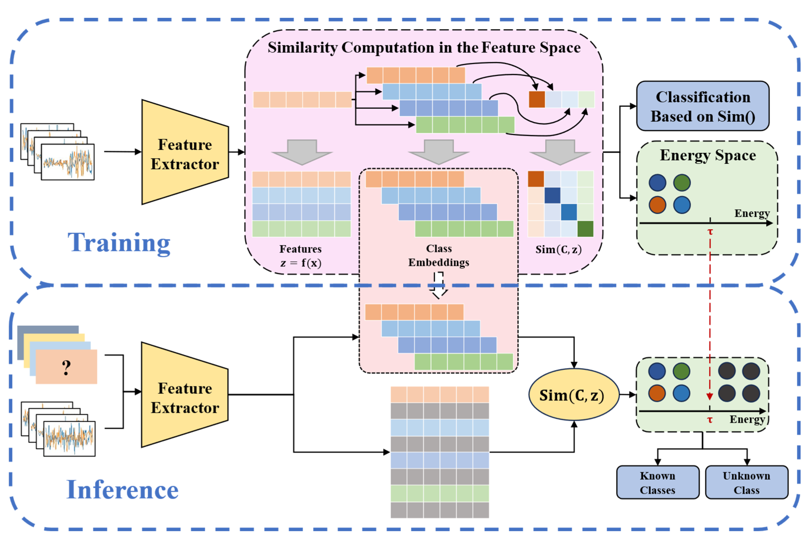
Figure 6.
The data acquisition process.
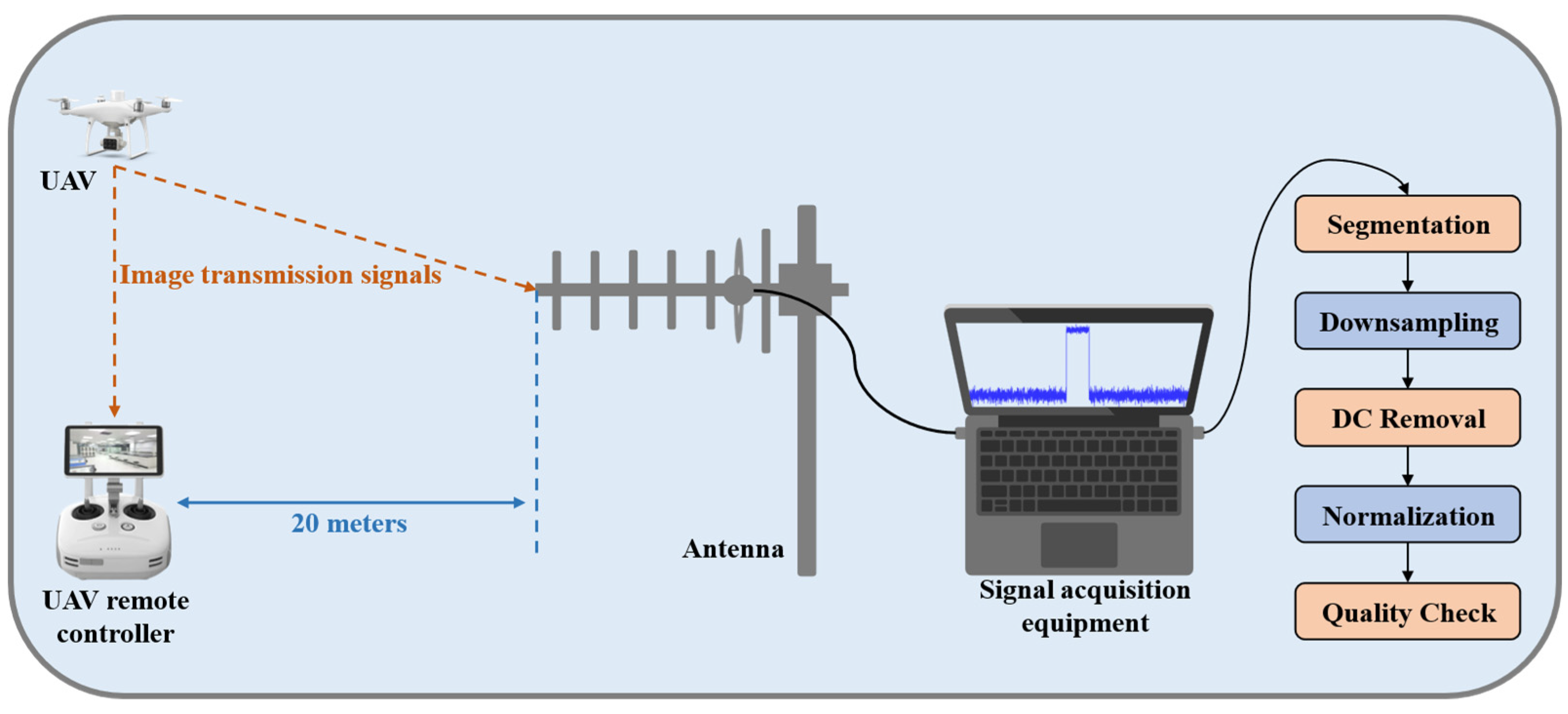
Figure 7.
Closed-set classification accuracy of different models under varying SNR conditions.
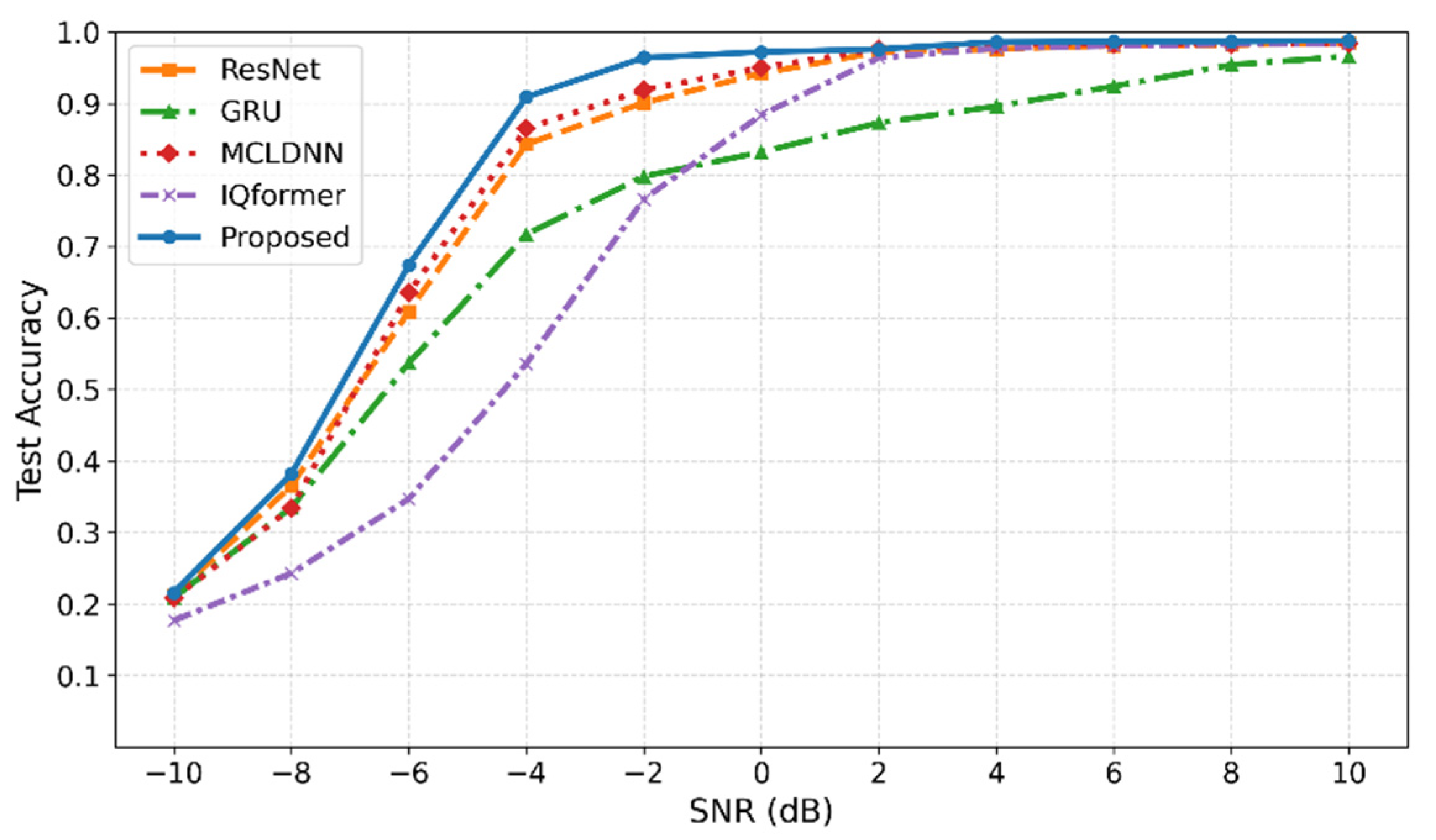
Figure 8.
Confusion matrices of different models at 0 dB SNR: (a) ResNet; (b) GRU; (c) MCLDNN; (d) IQformer; (e) Proposed model. The proposed approach shows greater diagonal dominance and fewer inter-class confusions than the baselines.
Figure 8.
Confusion matrices of different models at 0 dB SNR: (a) ResNet; (b) GRU; (c) MCLDNN; (d) IQformer; (e) Proposed model. The proposed approach shows greater diagonal dominance and fewer inter-class confusions than the baselines.
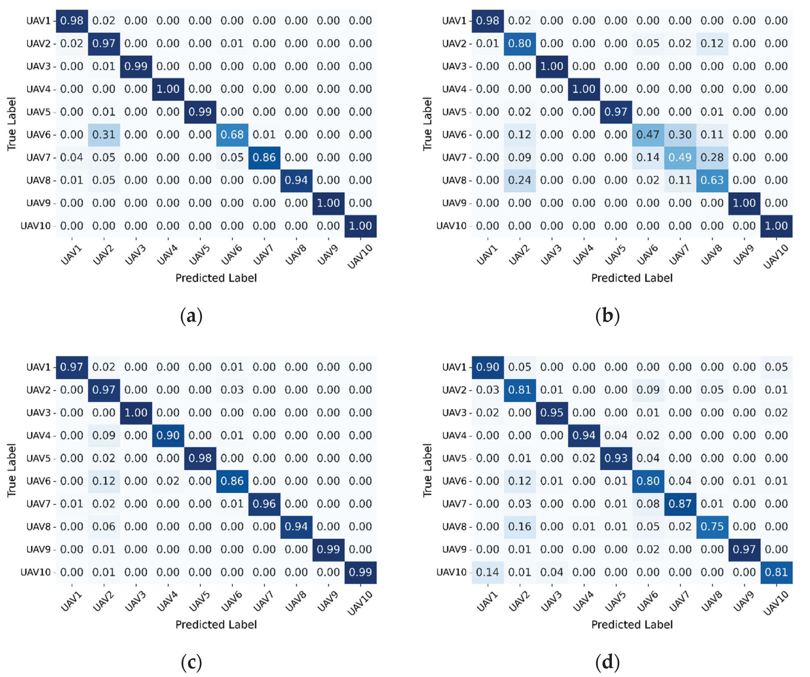
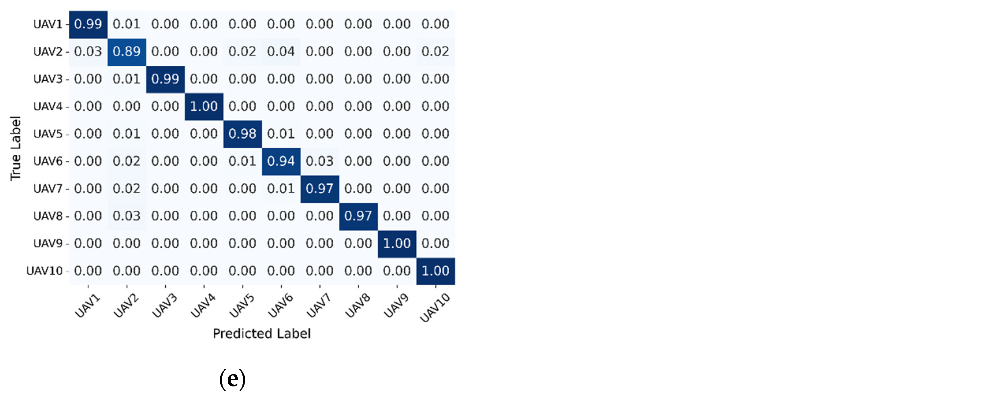
Figure 9.
t-SNE visualization of the feature space at 0 dB SNR: (a) ResNet; (b) GRU; (c) MCLDNN; (d) IQformer; (e) Proposed model. The proposed approach yields more compact, separable feature clusters than baseline networks.
Figure 9.
t-SNE visualization of the feature space at 0 dB SNR: (a) ResNet; (b) GRU; (c) MCLDNN; (d) IQformer; (e) Proposed model. The proposed approach yields more compact, separable feature clusters than baseline networks.
Figure 10.
OSCR performance curves of different methods under varying SNR conditions.
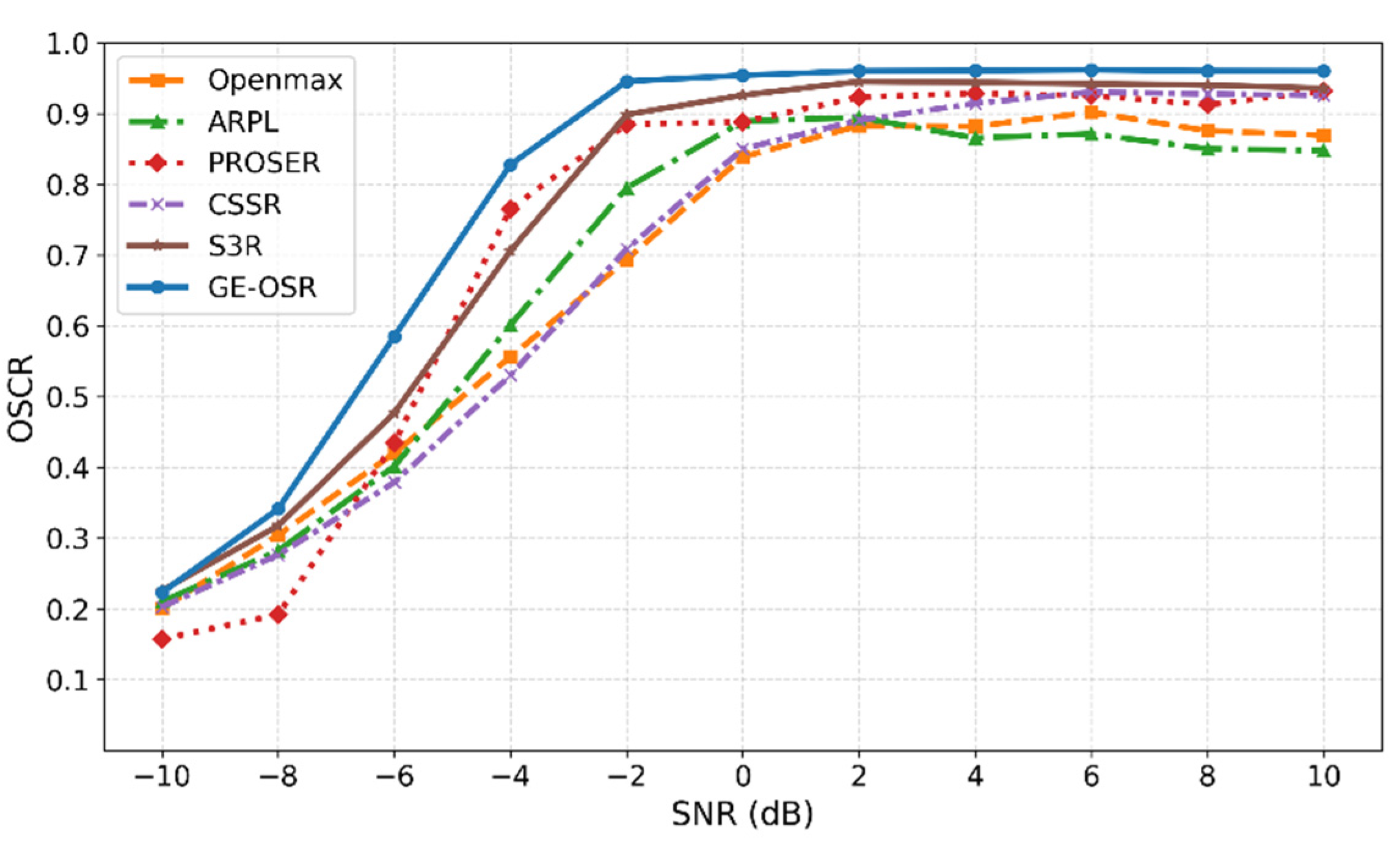
Figure 11.
Feature visualization of known and unknown classes across different open-set recognition methods: (a) OpenMax; (b) ARPL; (c) PROSER; (d) CSSR; (e) S3R; (f) Proposed GE-OSR. The proposed GE-OSR produces compact intra-class clusters and well-separated inter-class boundaries, effectively isolating unknown samples from known feature regions.
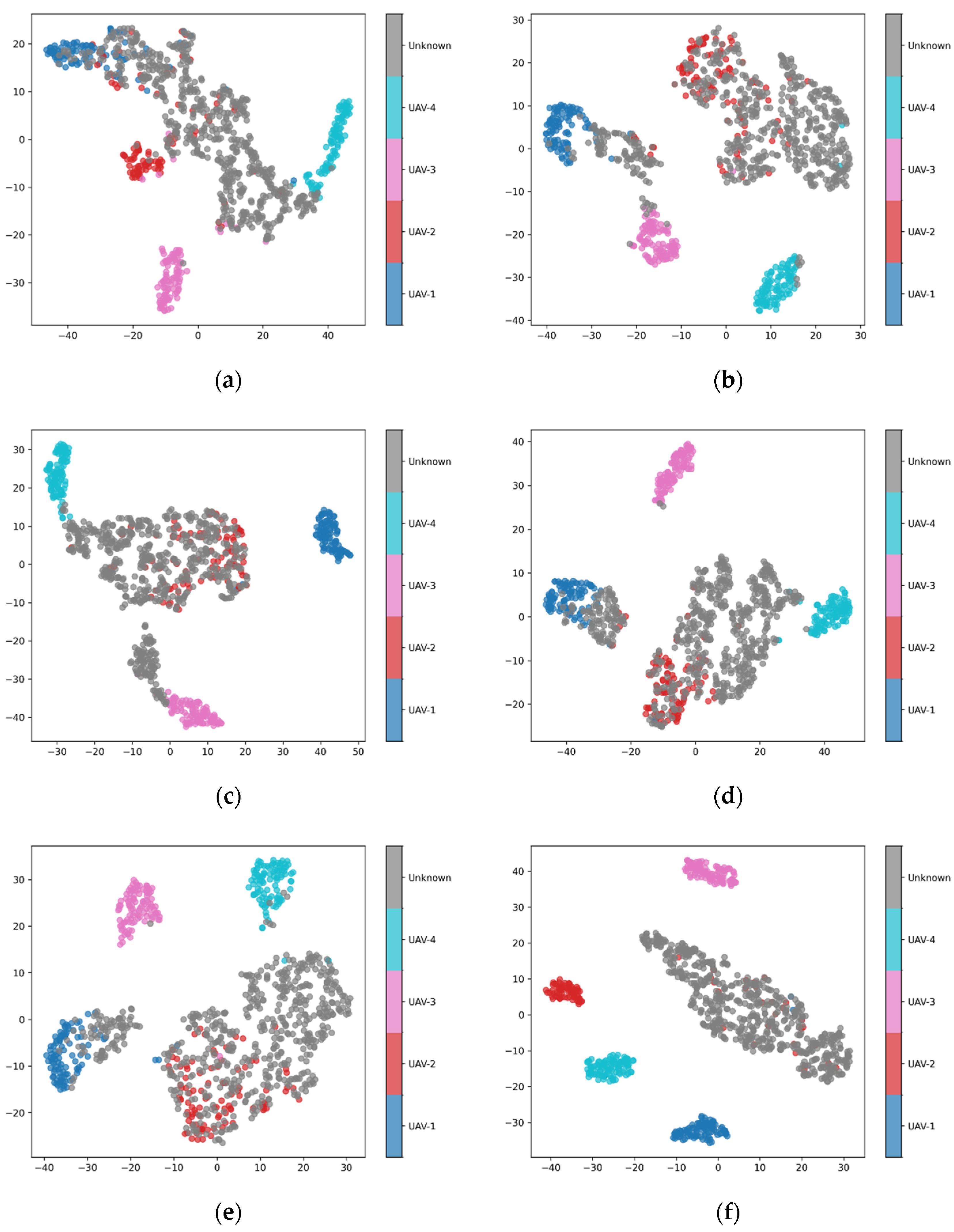
Figure 12.
Effect of threshold settings on open-set recognition performance: (a) Free energy distributions of known and unknown samples; (b) Accuracy-rejection rate curves across different thresholds.
Figure 12.
Effect of threshold settings on open-set recognition performance: (a) Free energy distributions of known and unknown samples; (b) Accuracy-rejection rate curves across different thresholds.
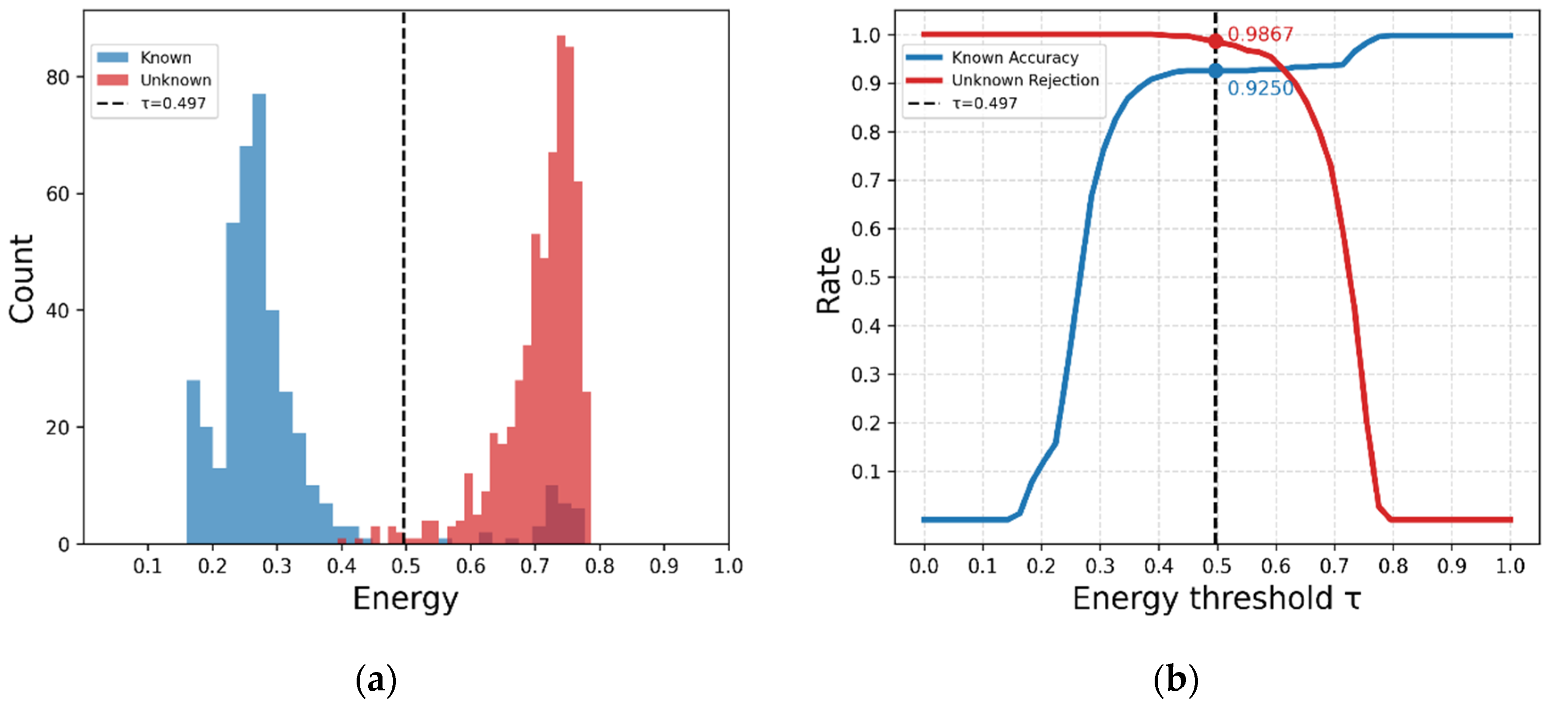
Figure 13.
Open-set recognition confusion matrix.
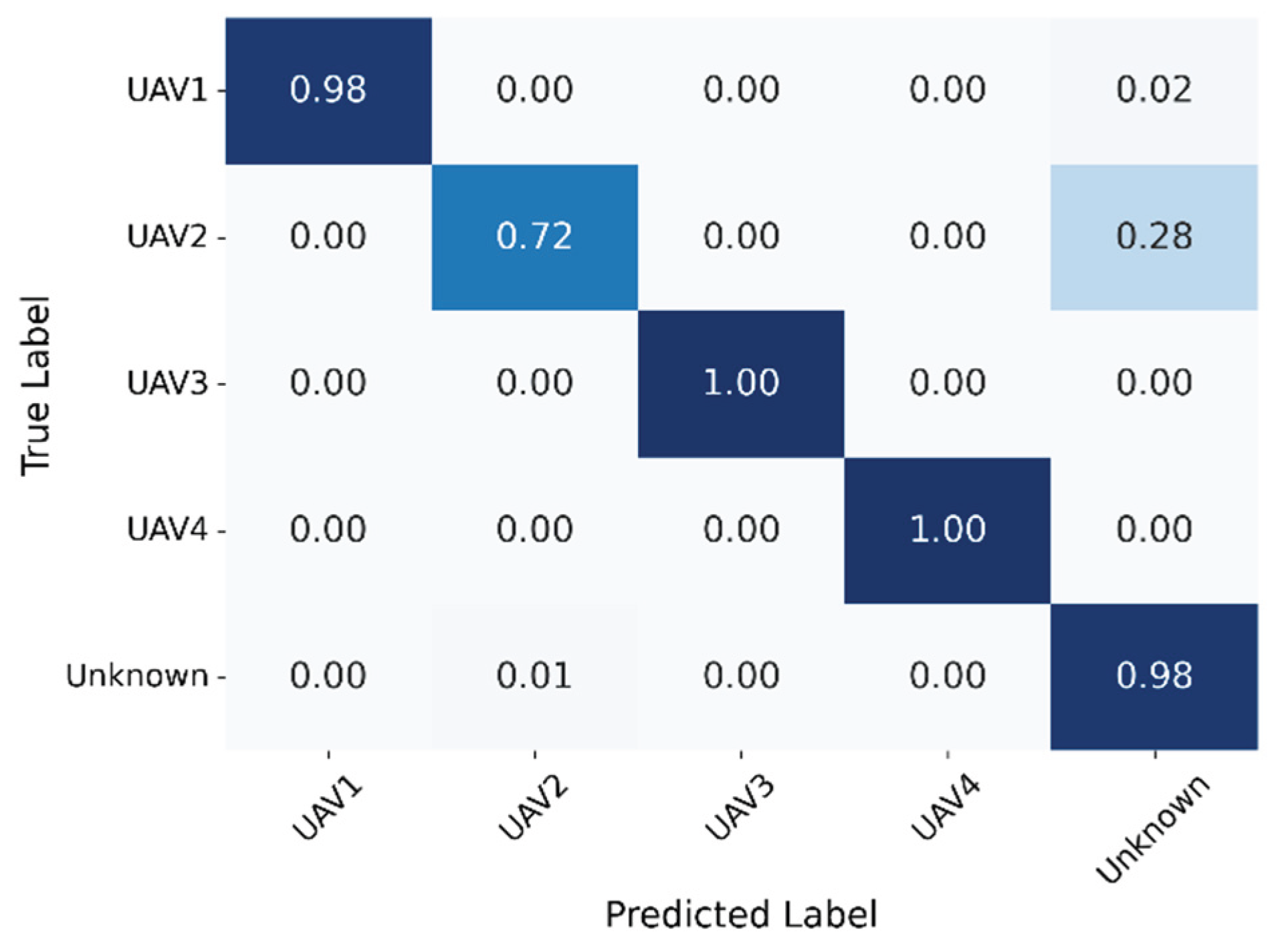

Table 1.
Experimental settings.
| Parameter | Value |
| 32 | |
| 0.1 | |
| 10.0 | |
| -0.1 | |
| 0.3 | |
| 1.0 | |
| 0.2 | |
| batch size | 128 |
| optimizer | AdamW |
| learning rate | 0.001 |
Table 2.
Closed-set classification performance of different models at 0 dB.
| Model | Parameters | Acc (%) | F1-score (%) |
| ResNet | 0.153M | 94.21 ± 1.13 | 94.30 ± 1.11 |
| GRU | 0.159M | 83.24 ± 1.91 | 83.02 ± 2.08 |
| MCLDNN | 0.241M | 95.04 ± 0.98 | 95.14 ± 1.13 |
| IQformer | 0.072M | 88.37 ± 0.36 | 88.38 ± 0.41 |
| Proposed | 0.062M | 97.19 ± 0.55 | 97.20 ± 0.62 |
Table 3.
AUROC (%) Results across Openness Levels (4 Known Classes, 0 dB SNR).
| Method | Number of Unknown Classes | Average | |||||
| 1 | 2 | 3 | 4 | 5 | 6 | ||
| Openmax | 96.80 ± 0.77 | 94.05 ± 1.03 | 93.32 ± 1.21 | 91.64 ± 1.54 | 88.82 ± 1.47 | 87.75 ± 1.82 | 92.06 ± 3.37 |
| ARPL | 97.65 ± 0.93 | 92.93 ± 2.80 | 93.45 ± 2.14 | 91.69 ± 3.57 | 92.18 ± 2.69 | 89.62 ± 0.76 | 92.92 ± 3.40 |
| PROSER | 93.51 ± 1.50 | 89.62 ± 2.55 | 90.73 ± 2.13 | 90.19 ± 2.30 | 90.36 ± 2.15 | 89.61 ± 0.31 | 90.67 ± 2.38 |
| CSSR | 96.57 ± 0.34 | 92.96 ± 1.06 | 93.29 ± 1.43 | 91.98 ± 1.85 | 89.41 ± 0.39 | 87.95 ± 2.76 | 92.02 ± 3.19 |
| S3R | 97.49 ± 0.98 | 95.15 ± 0.90 | 95.34 ± 1.33 | 95.00 ± 0.76 | 94.81 ± 1.01 | 93.32 ± 0.68 | 95.18 ± 1.56 |
| GE-OSR | 98.19 ± 0.93 | 97.04 ± 0.69 | 96.55 ± 0.72 | 96.53 ± 0.69 | 96.56 ± 0.95 | 96.39 ± 0.56 | 96.87 ± 0.99 |
Table 4.
OSCR (%) Results across Openness Levels (4 Known Classes, 0 dB SNR).
| Method | Number of Unknown Classes | Average | |||||
| 1 | 2 | 3 | 4 | 5 | 6 | ||
| Openmax | 95.24 ± 0.22 | 93.07 ± 0.47 | 90.77 ± 0.34 | 89.39 ± 0.61 | 85.70 ± 1.37 | 83.86 ± 1.00 | 89.67 ± 4.02 |
| ARPL | 96.67 ± 0.92 | 92.13 ± 2.81 | 92.81 ± 2.31 | 91.14 ± 3.74 | 91.75 ± 2.61 | 88.91 ± 0.94 | 92.23 ± 3.37 |
| PROSER | 92.24 ± 2.43 | 88.70 ± 2.90 | 89.43 ± 2.51 | 89.34 ± 2.42 | 89.58 ± 2.59 | 88.80 ± 0.28 | 89.68 ± 2.64 |
| CSSR | 95.39 ± 0.73 | 91.63 ± 1.21 | 92.34 ± 1.66 | 90.84 ± 1.94 | 88.59 ± 0.63 | 85.01 ± 1.84 | 90.63 ± 3.53 |
| S3R | 96.62 ± 1.14 | 94.31 ± 1.12 | 94.67 ± 1.47 | 94.42 ± 0.79 | 94.25 ± 1.14 | 92.84 ± 0.70 | 94.52 ± 1.56 |
| GE-OSR | 96.85 ± 0.84 | 96.19 ± 0.73 | 95.98 ± 0.79 | 95.93 ± 0.89 | 95.84 ± 0.93 | 95.39 ± 0.67 | 96.03 ± 0.92 |
Table 5.
Ablation study of GE-OSR.
| TFFM | DCEL | FEAL | AUROC (%) | OSCR (%) |
| × | × | × | 70.09 ± 1.80 | 62.35 ± 1.34 |
| √ | × | × | 84.57 ± 0.70 | 82.07 ± 0.39 |
| √ | √ | × | 89.50 ± 1.68 | 88.85 ± 1.36 |
| √ | √ | √ | 96.39 ± 0.56 | 95.39 ± 0.67 |
Disclaimer/Publisher’s Note: The statements, opinions and data contained in all publications are solely those of the individual author(s) and contributor(s) and not of MDPI and/or the editor(s). MDPI and/or the editor(s) disclaim responsibility for any injury to people or property resulting from any ideas, methods, instructions or products referred to in the content. |
© 2025 by the authors. Licensee MDPI, Basel, Switzerland. This article is an open access article distributed under the terms and conditions of the Creative Commons Attribution (CC BY) license (http://creativecommons.org/licenses/by/4.0/).
Copyright: This open access article is published under a Creative Commons CC BY 4.0 license, which permit the free download, distribution, and reuse, provided that the author and preprint are cited in any reuse.


