
Submitted:
31 October 2025
Posted:
31 October 2025
You are already at the latest version
Abstract
In the field of remote sensing, tracking highly maneuvering targets is challenging due to its rapidly changing patterns and uncertainties, particularly under non-Gaussian noise conditions. In this paper, we consider the problem of tracking highly maneuvering targets without using preset parameters in non-Gaussian noise. We propose a multi-domain intelligent state estimation network (MIENet). It consists of two main models to estimate the key parameter for the Unscented Kalman Filter, enabling robust tracking of highly maneuvering targets under various intensities and distributions of observation noise. The first model, called fusion denoising model (FDM), is designed to eliminate observation noise by enhancing multi-domain feature fusion. The second model, called parameter estimation model (PEM), is designed to estimate key parameters of target motion by learning both global and local motion information. Additionally, we design a physically constrained loss function (PCLoss) that incorporates physics-informed constraints and prior knowledge. We evaluate our method on radar trajectory simulation and real remote sensing video datasets. Simulation results on the LAST dataset demonstrate that the proposed FDM can reduce the root mean square error (RMSE) of observation noise by more than 60\%. Moreover, the proposed MIENet consistently outperforms the state-of-the-art state estimation algorithms across various highly maneuvering scenes, achieving this performance without requiring adjustment of noise parameters under non-Gaussian noise. Furthermore, experiments conducted on the real-world SV248S dataset confirm that MIENet effectively generalizes to satellite video object tracking tasks.
Keywords:
multi-domain intelligent estimation
; fusion denoising
; parameter estimation
; nonlinear filtering system
1. Introduction
In the context of Earth observation (EO), target tracking aims to estimate target states from noisy EO measurements acquired by satellite, radar, and UAV sensors. It supports UAV object tracking [1,2,3,4], remote sensing surveillance [5,6,7], and traffic control [8,9,10]. Within the domain of target tracking, the problem of tracking highly maneuvering targets is widely recognized as a fundamental challenge [11,12,13]. Specially, highly maneuvering targets are characterized by motion involving high speeds, frequent maneuvers, and long-duration maneuvers. Tracking such targets presents two main challenges. The first challenge is high-speed and high-frequency maneuvers [14]. Such maneuvers cause rapid motion changes and result in error accumulation. The second challenge arises from non-Gaussian noise with different intensities and distributions [12], causing instability in state estimation results and divergence in tracking performance. Currently, multiple paradigms have been proposed to solve these challenges. They can be classified into two types, which are model-based methods and data-driven methods.
For model-based methods [15,16,17,18,19,20,21], the interacting multiple model (IMM) filter [19] is a fundamental algorithm to solve rapidly changing patterns problem [22]. It combines several predefined motion models and works with the improved Kalman filter [15,17,23,24,25,26,27,28,29] to achieve reliable tracking in nonlinear systems. To enhance adaptability under non-Gaussian noise, Xu et al. [30] proposed an EM-based extended Kalman filter (EKF) tracker that decomposed non-Gaussian noise into Gaussian components and incorporated bias compensation, significantly improving angle-of-arrival target tracking under non-Gaussian noise conditions. Building on the idea of Gaussian decomposition, Chen et al. [31] proposed a joint probability data association based on noise-interaction Kalman filter (JPDA-IKF), which decomposed non-Gaussian noise into multiple Gaussian components and fused their results to enhance multitarget tracking performance in complex maritime environments. To further capture multimodal noise and motion characteristics, Wang et al. [32] introduced Gaussian mixture models (GMMs) into the IMM-KF, allowing accurate switching and fusion across multiple motion. Liu et al. [33] proposed an IMM-MCQKF algorithm that integrated the maximum correntropy criterion into the quadrature Kalman filter within an IMM framework, improving state estimation under non-Gaussian noise and maneuvering target scenarios. Xie et al. [34] proposed an adaptive TPM-based parallel IMM algorithm that integrated online transition probability adaptation with a threshold-controlled model-jumping mechanism within the IMM framework.
The above model-driven methods require accurate motion patterns and covariance noise parameters based on manual experiences. Indeed, constructing an accurate and well-matched model is challenging, and such prior information cannot be obtained promptly and reliably before tracking [22]. Additionally, these methods process trajectories only in the temporal domain and do not fully exploit multi-domain information. As a result, by neglecting the latent representational information in noisy observations, their sensitivity to maneuverability is reduced under non-Gaussian noise.
For data-driven methods, precise kinematic modeling of target motion is unnecessary. They leverage the strength of data mining to capture complex dynamics. They can be broadly categorized into two types, which are end-to-end architectures and hybrid architectures that integrate traditional algorithm. The former constructs an end-to-end model to directly map the input observations to the output states, eliminating the need for manually designed intermediate feature extraction. Cai et al. [35] proposed an adaptive LSTM-based tracking method that incorporated measurement–prediction errors to improve accuracy and adaptability for maneuvering targets. Liu et al. [11] learned the residual between the ground truth and estimation trajectories. This framework mainly consisted of BiLSTM layers [36,37,38] and enabled target state estimation without the need for a pre-defined model set. Building upon these, Zhang et al. [13,39] employed an enhanced transformer architecture to achieve further reductions in state estimation RMSE. Shen et al. [40] also proposed Transformer-based nonlinear target trackers, including a classical Transformer for smoothing and prediction and a recursive Transformer for filtering and prediction, achieving superior accuracy and efficiency in nonlinear radar target tracking. PCRLB [41] propose a physics-informed data-driven autoregressive nonlinear filter (DAF) based on the Transformer. Its end-to-end architecture embedded known dynamics and measurement models into the training process, ensuring physically consistent and efficient state estimation.
The above end-to-end data-driven methods primarily use a single end-to-end model to capture complex nonlinear functions often leads to convergence difficulties in practice. Moreover, a wide variation range of target motion may degrade method performance and generalization.
The latter hybrid methods [12,42,43,44,45,46,47,48,49,50,51,52,53,54,55,55] integrate deep learning with model-driven approaches, thereby combining the strengths of both paradigms. These methods retain the framework of model-driven algorithms while incorporating deep learning modules to estimate variable parameters. By involving less functional learning and relying on simpler architectures, they achieve lower computational cost and enhanced interpretability. KalmanNet [42] integrated a structural state space model with dedicated recurrent neural networks (RNN) to estimate the Kalman gain. It operated within the KF framework and effectively addressed non-linearity. Building on this idea, KalmanFormer [53] employed a Transformer to learn the Kalman Gain. To handle mismatches between state and observation models, Split-KalmanNet [43] calculated the Kalman gain through the Jacobian of the measurement function and leveraged two RNNs with a split architecture. Cholesky-KalmanNet [45] further enhances state estimation by providing and enforcing transiently precise error covariance estimation. Recursive KalmanNet [48] extended this line of research by employing the recursive Joseph’s formulation, thereby enabling accurate state estimation with consistent uncertainty quantification under non-Gaussian noise. Latent-KalmanNet [44] advanced the framework by jointly learning a latent representation and Kalman-based tracking from high-dimensional signals. More recently, MAML-KalmanNet [54] integrated model-agnostic meta-learning with artificially generated labeled data to achieve fast adaptation and accurate state estimation under partially unknown models. In addition, Liu [12] introduced a digital twin system that combined the Unscented Kalman filter with intelligent estimation models. Zhu [56] developed an adaptive IMM algorithm that employed a neural network to estimate TPMs in real time, thereby reformulating IMM as a generalized recurrent neural network. Fu [46] proposed deep learning–aided Bayesian filtering methods for guarded semi-Markov switching systems with soft constraints, addressing the challenge of state estimation under complex sojourn times and state-dependent transitions. Furthermore, Jia [50] proposed a Multiple Variational Kalman-GRU model to capture multimodal ship dynamics and provide reliable trajectory prediction.
This paradigm endows the network with stronger generalization ability and interpretability. Considering these advantages, we adopt this paradigm in our work. However, existing hybrid approaches that integrate deep learning into traditional model-driven frameworks still have notable limitations. They typically rely solely on temporal-domain processing and fail to exploit complementary information from spatial and frequency domains, thereby restricting their effectiveness. In addition, when dealing with maneuvering targets, these methods often emphasize local temporal features while overlooking broader global motion patterns, which are critical for capturing abrupt changes in dynamics.
To overcome these issues, we propose a versatile and adaptive tracking framework called the Multi-Domain Intelligent State Estimation Network (MIENet) for highly maneuvering target tracking that can effectively handle non-Gaussian noise. MIENet first applies a nonlinear transformation for coordinate system conversion and comprises two main models. Due to the nonlinear, heavy-tailed, and spatially correlated characteristics of non-Gaussian noise, standard Gaussian-based methods fail to remove it effectively. The independent module in MIENet enables adaptive learning of these complex noise features, thereby improving convergence stability and denoising efficiency. Furthermore, leveraging multi-domain information helps capture the statistical characteristics of non-Gaussian noise. Therefore, the first model, termed the Fusion Denoising Model (FDM), mitigates non-Gaussian observation noise by integrating temporal, spatial, and frequency-domain features.
As discussed in [12], bias in causes rapidly growing deviations, while bias in the initial state results in linear growth. Hence, errors from an inaccurate transition matrix become much greater than those from an incorrect initial state as the trajectory extends. The main challenge in estimating the maneuvering target motion model lies in the uncertainty of , whose exact form is typically unknown; thus, accurately estimating its key parameters is critical to avoid computational bias. Motivated by this, the second model, termed the Parameter Estimation Model (PEM), estimates the turn rate of target motion from temporal–spatial information. The estimated parameters are then incorporated into the UKF to achieve accurate tracking of highly maneuvering targets. The entire tracking process is iteratively updated using a fixed sliding-window mechanism. The main contributions of this work are summarized as follows:
- We propose a MIENet to estimate target state and motion patterns from non-Gaussian observation noise. The multi-domain information of target trajectories can be well incorporated, thus helping to infer the latent state of targets.
- We design a FDM to handle noise with varying intensities and distributions. It employs a novel Inverted-UNet and FFT-based weighting to integrate temporal, spatial, and frequency-domain features within an encoder–decoder framework.
- We develop a PEM to estimate target motion patterns by fusing local and global spatial–temporal features. Considering that the state transition matrix () characterizes motion dynamics and enables trajectory inference, we further introduce a physically constrained loss function (PCLoss) to help PEM estimate the key turn rate parameter () in .
2. Problem Formulation
Our method is dedicated to maneuvering target tracking and shows limited dependence on the observation modality. Using the LAST dataset as an example, we analyze a radar tracking system. As shown in Figure 1, the system structure is based on range and azimuth observations [12]. Initially, due to the long distance of the target and the limited measurement resolution, we ignore the shape of targets and treat them as points in space [14]. The relationship of target states and observations is represented by the state space model (SSM) as follows,
where and are target states and observations at time step k, respectively. is defined as , where is the two-dimensional position, and is the corresponding velocity. is defined as , where and are the range and azimuth of the target detected by the sensor. and are additive noise at time step k; and are the state transition matrix and observation function.
2.1. State Equation
For most 2D maneuvering tracking scenes, Constant Turn (CT) models [14] are representative maneuvering patterns that can approximate most motion behaviors. The is defined as:
where denotes the turn rate at time step k. It is a critical parameter whose accuracy significantly affects performance. The symbol represents the sampling interval of trajectories. If equals to zero, the motion model is simplified to Constant Velocity (CV) model, which could be defined as:
2.2. Observation Equation
For common radar tracking system, the detector at provides range and azimuth measurements contaminated by additive noise. The polar coordinate system of observations is given as:
where and are additive noise in range and azimuth angle observations at time step k.
Subsequently, The polar coordinate system is transformed into the Cartesian system as the input of our method. In this step, additive noise is converted into non-Gaussian noise by nonlinear transformation. The process is formulated as follows:
2.3. Problem Addressed in This Work
The main task is to estimate the target states () based on the nonlinear observation (). This work addresses two primary challenges. First, the observations are often corrupted by diverse types of noise. In practice, for nonlinear observations, the noise distributions we processed are rarely Gaussian; instead, they may vary in intensity, exhibit non-Gaussian characteristics, or change dynamically across different environments. Second, maneuvering targets introduce additional difficulties due to their highly dynamic and uncertain motion patterns. A key challenge lies in accurately estimating critical motion parameters in the state transition matrix (). Errors in estimating such parameters can severely degrade trajectory inference, as the deviation induced by model mismatch often grows increasingly with trajectory length. This work aims to design a robust framework for stable and reliable tracking of highly maneuvering targets. The framework can effectively handle non-Gaussian noise and accurately estimate key motion parameters.
3. Multi-Domain Intelligent State Estimation Network
In this work, we introduce our MIENet in details. The overall architecture of the proposed method is shown in Figure 2.
3.1. Overall Architecture
As illustrated in Figure 2, we segment the acquired trajectories using a sliding window, and our MIENet processes fixed-length noisy polar-coordinate trajectories as input. It first applies a nonlinear transformation (Equation (6)) to convert polar coordinates () into Cartesian coordinates (). In this process, additive noise is transformed into non-Gaussian noise. A fusion denoising model (FDM, Section 3.2) is then employed to suppress non-Gaussian observation noise by integrating temporal, spatial, and frequency-domain features. Subsequently, a parameter estimation model (PEM, Section 3.3) estimates the turn rate from the denoised trajectories output by the FDM. It leverages both local and global temporal–spatial information. The estimated parameter is then incorporated into a UKF for maneuvering target tracking. Notably, the FDM and PEM are trained independently and evaluated jointly with the UKF in testing. A summary of the overall tracking process is provided in Algorithm 1. Subsequently, the FDM and PEM are described in detail.
| Algorithm 1 MIENet tracking process |
|
3.2. Fusion Denoising Model
3.2.1. Motivation
In practice, the statistical characteristics of observation noise exist not only in the temporal domain but also in the spatial and frequency domains. Temporal features alone are insufficient to capture oscillatory energy distributions in the frequency domain or spatial structural correlations, both of which are essential for robust denoising and stable tracking under non-Gaussian noise.
As noted in [58], the encoder-decoder structure enables effective separation of noise and signal in the latent space, ensuring noise suppression during reconstruction. However, traditional encoder-decoder structure consists of an encoder, a decoder, and plain connections. The encoder is used to increase feature dimension while reducing the spatial resolution. Decoder helps to recover the spatial resolution to match the size of input trajectories. Such architectures mainly emphasize hierarchical semantic features derived from temporal information. Although deepening the network or modifying the encoder submodules can capture higher-level representations, they do not explicitly address the multi-domain characteristics of observation noise. This motivates the design of a dedicated module within the encoder–decoder framework to explicitly extract and fuse temporal, spatial, and frequency-domain features.
3.2.2. The Overall Structure of FDM
As illustrated in Figure 3, the framework adopts a symmetric encoder–decoder structure with an additional multi-domain feature module (MDFM). The input trajectories are converted from polar to Cartesian coordinates and segmented into fixed-length sequences. These processed sequences are subsequently fed into the transformer encoder to extract temporal-domain features. The MDFM further captures frequency-domain and spatial-domain information, and fuses them with temporal dynamics. Finally, the fused multi-domain features are passed into the decoder subnetworks for trajectory reconstruction and prediction.
3.2.3. The Multi-Domain Feature Module
As shown in Figure 3, the multi-domain feature module (MDFM) is embedded within the encoder to enhance feature representation beyond the temporal domain. It first performs padding and reshaping on the input data, and then passes it through the Inverted-UNet. The Inverted-UNet is specifically designed to capture both multi-channel spatial structures while maintaining computational efficiency, which is critical for robust trajectory representation. The extracted features are then normalized with Layer Normalization and activated by a LeakyReLU, with this block repeated p times according to experimental results.
In parallel, the Fast Fourier Transform (FFT) is applied to the temporal features to reveal frequency-domain amplitude distributions. These amplitudes are used as weights, allowing the model to emphasize oscillatory patterns that are often hidden in noisy observations. The denoised spatial features from the Inverted-UNet and the weighted frequency-domain information are fused through a softmax layer.
By combining the Inverted-UNet and FFT, MDFM explicitly leverages spatial structures and frequency-domain energy patterns, providing a more comprehensive feature representation that significantly improves noise suppression. The following sections present a detailed description of these two key components.
- (1)
- The Inverted-UNet
For low-dimensional trajectory sequences, the traditional dense U-Net (Figure 4(a)) is unsuitable, as its initial downsampling step leads to an immediate loss of information. Based on this idea, we design a novel Inverted-UNet (Figure 4(b)). It first upsamples the multi-channel trajectory features to preserve spatial structure, then downsamples them to restore the original trajectory shape. Skip connections promote gradient flow.
Assume denotes the output of each node, where i is the upsampling layer in the encoder and j is the neighboring layer. To balance network performance and computational efficiency, the Inverted-UNet is designed with a depth of four layers, where the indices i and j take values from 0 to 3. The computation of each node feature is illustrated as follows,
where and denote upsampling and max-pooling with a stride of 2, respectively; denotes the convolution layer. denotes skip connection. denotes the concatenation layer.
- (2)
- FFT-Based Weighting
We apply Fast Fourier Transform (FFT) to extract their spectrum amplitude distribution. These serve as weights in the softmax layer to fuse different features. This approach utilizes temporal and frequency domains information to assess the importance of different signals. The process is illustrated as follows,
where represents the fixed-length input trajectory segment of the MDFM, generated through a sliding window mechanism. f denotes the frequency index, N is the length of each fixed trajectory segment, and n refers to the time-domain sampling index. The operator computes the magnitude in the frequency domain. denotes the output feature, which is subsequently processed by the Inverted-UNet, LayerNorm, and LeakyReLU modules in sequence.
3.3. Parameter Estimation Model
3.3.1. Motivation
In most 2D maneuvering tracking scenes, constant Turn (CT) models are important maneuvering patterns [11,12,14], where the motion pattern and its turn rate () are defined in Equation (3). The changing turn rate of a target affects the direction of its trajectory. Short-term trajectory features reflect instantaneous velocity variations and local motion trends, whereas long-term features characterize the overall motion pattern and the magnitude of velocity. Therefore, parameter estimation based on historical trajectory information requires a special module to extract both global and local spatial features.
As noted in [59], despite achieving accurate predictions with large-scale training data, networks still struggle to acquire inductive biases aligned with the underlying world model when adapting to new tasks. To address this limitation, the loss function becomes a crucial mechanism for embedding physical constraints into the learning process. Therefore, in our work, the PEM loss function should be designed to ensure that complies with physical laws and avoids calculation bias in the network output.
3.3.2. The Overall Structure of PEM
As illustrated in Figure 5, PEM takes a denoised trajectory as input. It first uses a cross-and-dot-product (CADP) [12] to extract trajectory shape information by calculating the sine and cosine of the intersection angle. The equations are shown below:
where , , .
Subsequently, the trajectory shape information is fed into multi-head attention with convolution neutral nodes (MHCN) to capture both global and local features from temporal and spatial domains. The attention output is fused with the original CADP features via a residual connection, and the result is further refined by convolutional neural nodes. Specially, a novel physically constrained loss function is applied during training to avoid bias in computing .
3.3.3. Physics-Constrained Loss Function
Considering the loss function design, we impose constraints on to enforce consistency with physical motion dynamics, thereby preventing the network from producing biased or physically implausible estimates. The estimation focuses on the key unknown parameter (the turn rate ) to minimize loss values. This approach enables PEM to directly obtain the time-to-time variation of the turn rate. Moreover, it could avoid calculation bias and achieve maneuvering target tracking at a higher turn rate (typically >10°/s, e.g. Transport Aircraft [60]). However, estimating only a single parameter as the loss is insufficient, as it may lead to a large search space and cause network divergence. Therefore, we further introduce computational constraints on . RMSE [11] measures the error between estimated parameters and their true values, serving to construct the loss function as follows:
where and are estimated parameters, and and are real parameters. and represent distinct loss weights set to 0.8 and 0.2, respectively.
4. Experiments
In this section, we first introduce our training protocol. Then, we compare our MIENet to several state-of-the-art state estimation methods. Finally, we present ablation studies to investigate our work.
4.1. Implementation Details
Our MIENet is trained using the publicly available LAST dataset [11], and the implementation details are provided in Table 1. For testing, we primarily evaluate our method on the LAST dataset [11], while experiments on the SV248S dataset [57] are provided as supplementary validation to demonstrate its applicability to visual tracking.
For training on the LAST datasets [11], all trajectories involve both CV and CT kinetic patterns. The observed range in training data contains additive Gaussian noise with a mean of 0 and a standard deviation of 10, while the observed azimuth contains additive Gaussian noise with a mean of 0 and a standard deviation of 0.006. After nonlinear transformation (Equation (6)), the observation noise becomes non-Gaussian. We use RMSE as the evaluation metric for the network performance. Our MIENet was trained with a batch size of 10, using the Adam optimizer with an initial learning rate of 0.01. To prevent the network from converging to a local minimum, the learning rate was adjusted using the Cosine Annealing method. All experiments were conducted on an NVIDIA 4090 GPU.
For testing on the LAST dataset [11], detailed parameter settings of testing scenes are provided in the caption of Table 2. We perform highly maneuvering scenes where is more than 10°/s (e.g. Transport Aircraft [60]) and each part has a maneuvering time exceeding 20 seconds. Specially, they also include abrupt turn rates (e.g., from -30°/s to 70°/s). Specifically, in the first test scene, the target is more than 20km away from the radar sensor. The angular velocities gradually decrease, and the second segment lasts up to 52.6 seconds. This tracking scenario presents a greater challenge than those discussed in previous papers [11,12]. In the second scene, the initial state matches the first scene, but we change the direction of the turn rate and increase its value, with turns lasting up to 40 seconds in the first and third segments. In the third scene, the radar senor is closer to the target, within a range of less than 4.5km. In the forth scene, the turn rate changes are more significant in both magnitude and direction (from -30°/s to 70°/s, and then from 70°/s to -10°/s) compared to the previous three trajectories. The four scenes vary in terms of target distance and maneuvering capability, which highlights the diversity and comprehensive coverage of the evaluation environments.
For testing on the SV248S dataset [57], the observations are generated using the results of the STAR [62] method, since our approach does not rely on a detector or an acceleration module tailored for image processing. Under this formulation, the observed and estimated coordinates are directly comparable without any nonlinear transformation. We evaluate our method on all scenes included in the SV248S dataset, following the same evaluation protocol as STAR. The algorithm ranking is determined according to two criteria: the 5-pixel precision metric and the area under the curve (AUC) of the success plot, corresponding to the precision rate (PR) and success rate (SR), respectively [62].
4.2. Comparison to the State-of-the-Art (SOTA)
To demonstrate the superiority of our method, we compare our MIENet to several state-of-the-art (SOTA) methods, including traditional methods (UKF-A [61], IMM [19] combining multiple CT motion patterns) and deep learning-based methods (ISPM [12]).
4.2.1. Quantitative Results
- (1)
- The LAST Dataset
To objectively evaluate the tracker performance, we record the momentary RMSEs over 100 Monte Carlo simulations.
Quantitative results are shown in Table 3. The improvements achieved by our MIENet over traditional methods are significant. That is because, our MIENet can learn multi-domain features that are robust to scene variations and leverages both local and global information to capture latent motion patterns. In contrast, the traditional methods are usually designed for specific scenes (e.g., specific motion pattern and measurement environment). Moreover, as shown in Figure 6, we set each scene with three different noise levels. With the increase of noise, traditional methods suffer a dramatic performance decrease while our MIENet maintains accuracy. That is because, the performance of traditional methods rely heavily on manually chosen parameters (e.g., the process noise covariance and the measurement noise covariance ) and cannot adapt to various noise. It is worth noting that our method preserves error stability more effectively than traditional approaches when abrupt changes occur in turn rate direction or magnitude. Moreover, it remains robust as it does not require re-adjustment of the noise parameters ( and ) under changing environmental noise.
As shown in Table 3, the improvements achieved by MIENet over deep learning-based methods (i.e., ISPM) are obvious. That is because, we redesign FDM and PEM is optimized for highly maneuvering target tracking. The Inverted-UNet combined with FFT-based softmax weighting enables fusion of spatial and frequency domain information. The physics-constrained loss function can avoid calculation bias. Consequently, multi-domain information of trajectories can be maintained and fully learned in the network. In the tracking process, our MIENet takes 47.2ms per iteration and ISPM takes 11.3ms. Both algorithms are suitable for real-time applications.
- (2)
- The SV248S Dataset
Quantitative results are presented in Table 4 and Table 5. The proposed MIENet demonstrates applicability to remote visual tracking, effectively reducing localization errors across various target classes, difficulty levels, and attribute categories without requiring retraining. These results further indicate that our method can be readily extended to two-dimensional visual object tracking tasks.
4.2.2. Qualitative Results
- (1)
- The LAST Dataset
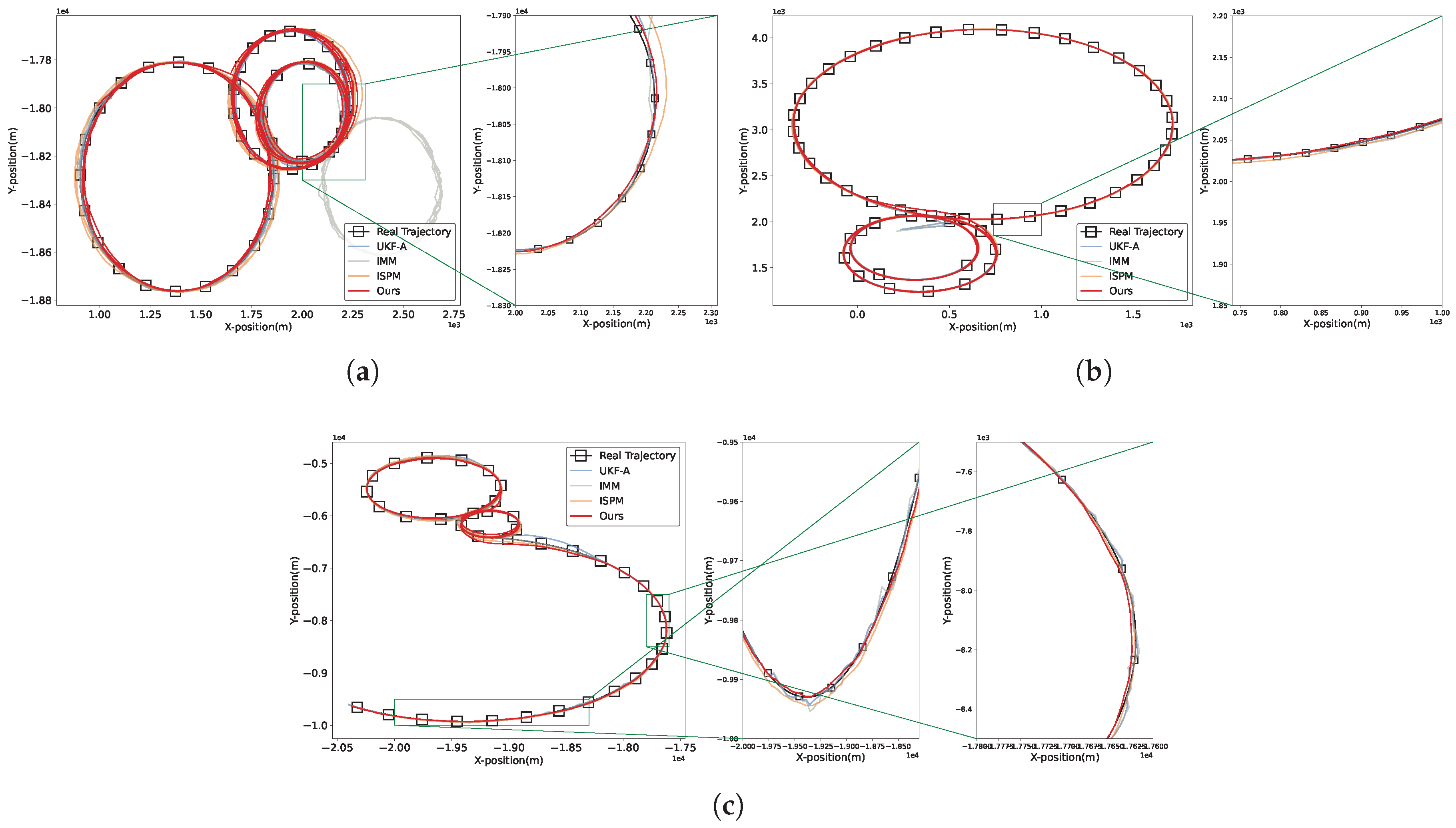
Qualitative results are shown in Figure 8. Compared with traditional methods, our method can produce output with precise target states and true velocity direction. Nonetheless, the traditional methods only perform well on low-noise scenes with slowly varying turn rates. Moreover, as shown in Figure 7b and Figure 7c, our MIENet can reduce peak tracking error. That is because, traditional methods detect pattern switching only after accumulating errors. This causes delay and peak error accumulation. The deep learning-based methods (i.e., ISPM) perform much better than traditional methods. However, due to highly maneuvering scenes, ISPM lacks multi-domain information and physical constraints, which leads to large parameter estimation errors. Our MIENet is more robust to various highly maneuvering target tracking.
Figure 7.
Trajectory estimation results for the first scene, along with the corresponding time-varying position and velocity errors. Our MIENet can achieve output with the lowest state estimation error and the smallest fluctuations.
Figure 7.
Trajectory estimation results for the first scene, along with the corresponding time-varying position and velocity errors. Our MIENet can achieve output with the lowest state estimation error and the smallest fluctuations.
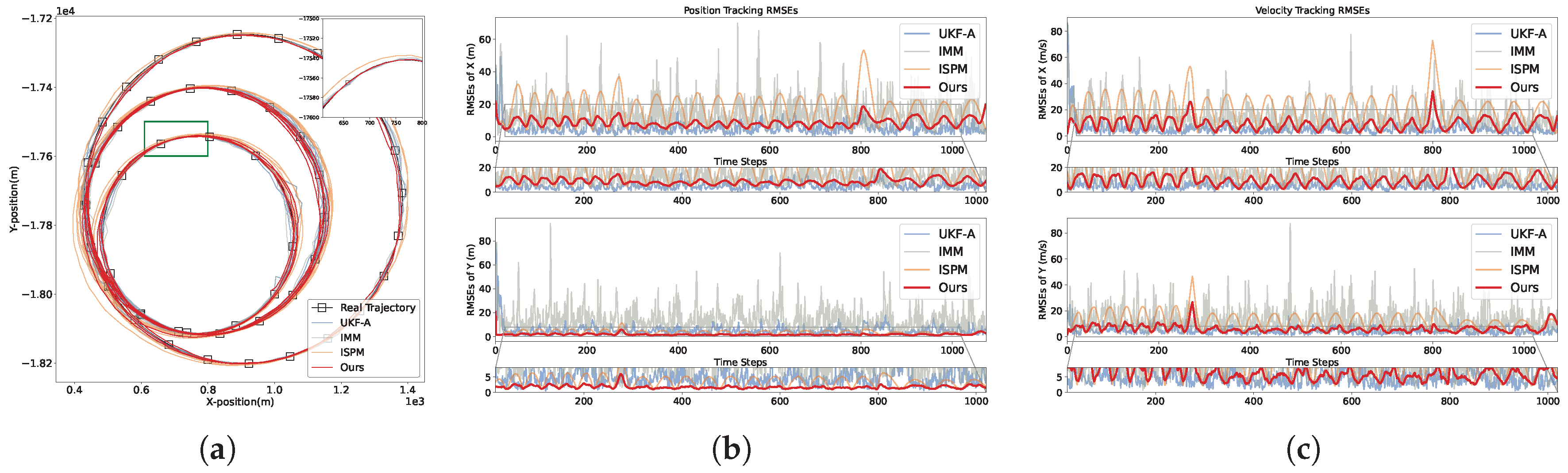
Figure 8.
Trajectory estimation results for the second, third, and fourth maneuvering target tracking scenarios. Our MIENet shows superior tracking accuracy, especially during periods of maneuvering transitions.
Figure 8.
Trajectory estimation results for the second, third, and fourth maneuvering target tracking scenarios. Our MIENet shows superior tracking accuracy, especially during periods of maneuvering transitions.
- (2)
- The SV248S Dataset
Qualitative results are shown in Figure 9. Our MIENet is capable of performing satellite localization in remote sensing images.
4.3. Ablation Study
In this section, we compare our MIENet with several variants. The objective is to investigate the potential benefits arising from our chosen modules and network design.
4.3.1. Ablation Study on the Magnitude and Distribution of Noise
As shown in Table 6 and Table 7, we evaluate the denoising performance under injected Gaussian-distributed and Uniform-distributed additive noise at three intensity levels to assess adaptability and generalization. Importantly, although the injected noise follows Gaussian or Uniform distributions in the input space, the nonlinear observation transformation distorts these distributions, producing non-Gaussian noise in the observation space.
Our method reduces RMSEs by at least 60% (with an average reduction of 66.4%) for cases with Gaussian-injected noise and at least 55% (with an average reduction of 63.28%) for cases with Uniform-injected noise. This consistent improvement demonstrates that FDM effectively exploits multi-domain information in observations, making it applicable to denoising tasks under varying noise levels and across different non-Gaussian noise distributions induced by nonlinear transformations.
4.3.2. Ablation Study on MDFM
MDFM is used for temporal, spatial and frequency-domain features enhancement to achieve better feature fusion. To investigate the benefits introduced by this module, we compare its effects on FDM and MIENet.
- FDM w/o MDFM: As shown in Table 8, the original FDM achieves a 61.2% reduction in RMSE, while removing the MDFM module decreases the reduction to 48.3%. The results are averaged over three noise intensity levels. This performance gap demonstrates that the Inverted-UNet is essential for denoising, as it extracts and fuses spatial-domain features more effectively from noisy observations.
- MIENet w/o MDFM: As shown in Table 9, our MIENet achieves position and velocity RMSEs of 7.78m and 10.64m/s, respectively. In ablation 1, removing the MDFM module increases RMSEs to 15.83m and 29.61m/s. That is because, FDM, as a component of MIENet, effectively suppresses noise and thereby contributes to its tracking performance.
4.3.3. Ablation Study on Multi-head Attention
We evaluate the contribution of multi-head attention (MHN) to MIENet and present the results in Table 9. In ablation 2, removing the MHN module increases RMSEs to 16.9m and 14.07m/s. That is because, our proposed MHN can capture historical global information about trajectories to enhance temporal domain features.
4.3.4. Ablation Study on Loss Function Design
The PCLoss function for PEM replaces the single parameter with eight unknown parameters. Results are shown in Table 9. Both Ablation 3 and our method demonstrate that the PCLoss function reduces the distance RMSE by 21.41% and the velocity RMSE by 21.47%. That is because, the PCLoss function can incorporate physical constrains and prevent bias in the calculations.
5. Conclusions
In this paper, we propose a versatile and adaptive multi-domain intelligent state estimation network to enhance highly maneuvering target tracking that can handle non-Gaussian noise. To address the challenges of converting noisy observation trajectories into clean inputs, we design FDM with an encoder-decoder architecture. This model enables reduction in RMSEs by at least 60% through exploiting multi-domain features. To achieve a more accurate motion model for state estimation, we propose PEM to capture temporal domain information across both global and local spatial scales. We also redesign the loss function to avoid calculation bias. Finally, experimental results demonstrate that our method achieves the state-of-the-art performance and maintains robustness across various noise levels and distributions.
There are two promising directions for future work. First, this paper considers only range and azimuth observations, incorporating Doppler measurements may further enhance maneuvering target tracking. Second, this work is restricted to tracking in the two-dimensional X–Y plane, extending the framework to three-dimensional scenarios is a valuable direction.
Author Contributions
Conceptualization, Z.M. and Y.H.; Methodology, Z.M. and Y.H.; Software, Z.M. and Q.X.; Validation, Z.M.; Investigation, Z.M., Q.X., W.A., X.W and W.S.; Visualization, Z.M., W.A. and Y.H.; Supervision, Y.H.; Project Administration, W.A.; Writing—Original Draft Preparation, Z.M., Y.H. and X.W.; Writing—Review and Editing, Y.H., Q.X., W.A., X.W. and W.S. All authors have read and agreed to the published version of the manuscript.
Funding
This work was supported in part by the National Natural Science Foundation of China under Grant 62207030; and in part by the Hunan Provincial Innovation Foundation for Postgraduate under Grant CX20240120.
Conflicts of Interest
The authors declare no conflicts of interest.
References
- Chen, Z.; Zhu, E.; Guo, Z.; Zhang, P.; Liu, X.; Wang, L.; Zhang, Y. Predictive Autonomy for UAV Remote Sensing: A Survey of Video Prediction. Remote Sensing 2025, 17, 3423. [Google Scholar] [CrossRef]
- Fraternali, P.; Morandini, L.; Motta, R. Enhancing Search and Rescue Missions with UAV Thermal Video Tracking. Remote Sensing 2025, 17, 3032. [Google Scholar] [CrossRef]
- Bu, D.; Ding, B.; Tong, X.; Sun, B.; Sun, X.; Guo, R.; Su, S. FSTC-DiMP: Advanced Feature Processing and Spatio-Temporal Consistency for Anti-UAV Tracking. Remote Sensing 2025, 17, 2902. [Google Scholar] [CrossRef]
- Zhou, Y.; Tang, D.; Zhou, H.; Xiang, X. Moving Target Geolocation and Trajectory Prediction Using a Fixed-Wing UAV in Cluttered Environments. Remote Sensing 2025, 17, 969. [Google Scholar] [CrossRef]
- Meng, F.; Zhao, G.; Zhang, G.; Li, Z.; Ding, K. Visual detection and association tracking of dim small ship targets from optical image sequences of geostationary satellite using multispectral radiation characteristics. Remote Sensing 2023, 15, 2069. [Google Scholar] [CrossRef]
- Huang, J.; Sun, H.; Wang, T. IAASNet: Ill-Posed-Aware Aggregated Stereo Matching Network for Cross-Orbit Optical Satellite Images. Remote Sensing 2025, 17, 3528. [Google Scholar] [CrossRef]
- Li, S.; Fu, G.; Yang, X.; Cao, X.; Niu, S.; Meng, Z. Two-Stage Spatio-Temporal Feature Correlation Network for Infrared Ground Target Tracking. IEEE Transactions on Geoscience and Remote Sensing 2024, 62, 1–14. [Google Scholar] [CrossRef]
- Zhao, D.; He, W.; Deng, L.; Wu, Y.; Xie, H.; Dai, J. Trajectory tracking and load monitoring for moving vehicles on bridge based on axle position and dual camera vision. Remote Sensing 2021, 13, 4868. [Google Scholar] [CrossRef]
- Xia, Q.; Chen, P.; Xu, G.; Sun, H.; Li, L.; Yu, G. Adaptive Path-Tracking Controller Embedded With Reinforcement Learning and Preview Model for Autonomous Driving. IEEE Transactions on Vehicular Technology 2025, 74, 3736–3750. [Google Scholar] [CrossRef]
- Chen, Z.; Liu, L.; Yu, Z. Towards Robust Visual Object Tracking for UAV With Multiple Response Incongruity Aberrance Repression Regularization. IEEE Signal Processing Letters 2024, 31, 2005–2009. [Google Scholar] [CrossRef]
- Liu, J.; Wang, Z.; Xu, M. DeepMTT: A deep learning maneuvering target-tracking algorithm based on bidirectional LSTM network. Information Fusion 2020, 53, 289–304. [Google Scholar] [CrossRef]
- Liu, J.; Yan, J.; Wan, D.; Li, X.; Al-Rubaye, S.; Al-Dulaimi, A.; Quan, Z. Digital Twins Based Intelligent State Prediction Method for Maneuvering-Target Tracking. IEEE Journal on Selected Areas in Communications 2023, 41, 3589–3606. [Google Scholar] [CrossRef]
- Zhang, Y.; Li, G.; Zhang, X.P.; He, Y. A deep learning model based on transformer structure for radar tracking of maneuvering targets. Information Fusion 2024, 103, 102120. [Google Scholar] [CrossRef]
- Li, X.R.; Jilkov, V.P. Survey of maneuvering target tracking. Part I. Dynamic models. IEEE Transactions on Aerospace and Electronic Systems 2003, 39, 1333–1364. [Google Scholar]
- Kalman, R.E. A new approach to linear filtering and prediction problems. 1960, 82, 35–45. [Google Scholar] [CrossRef]
- Cortina, E.; Otero, D.; D’Attellis, C.E. Maneuvering target tracking using extended kalman filter. IEEE Transactions on Aerospace and Electronic Systems 1991, 27, 155–158. [Google Scholar] [CrossRef]
- Julier, S.; Uhlmann, J.; Durrant-Whyte, H.F. A new method for the nonlinear transformation of means and covariances in filters and estimators. IEEE Transactions on Automatic Control 2000, 45, 477–482. [Google Scholar] [CrossRef]
- Gustafsson, F.; Gunnarsson, F.; Bergman, N.; Forssell, U.; Jansson, J.; Karlsson, R.; Nordlund, P.J. Particle filters for positioning, navigation, and tracking. IEEE Transactions on Signal Processing 2002, 50, 425–437. [Google Scholar] [CrossRef]
- Blom, H.A.; Bar-Shalom, Y. The interacting multiple model algorithm for systems with markovian switching coefficients. IEEE Transactions on Automatic Control 1988, 33, 780–783. [Google Scholar] [CrossRef]
- Sheng, H.; Zhao, W.; Wang, J. Interacting multiple model tracking algorithm fusing input estimation and best linear unbiased estimation filter. IET Radar Sonar and Navigation 2017, 11, 70–77. [Google Scholar] [CrossRef]
- Sun, Y.; Yuan, B.; Miao, Z.; Wu, W. From GMM to HGMM: An approach in moving object detection. Computing and Informatics 2004, 23, 215–237. [Google Scholar]
- Chen, X.; Wang, Y.; Zang, C.; Wang, X.; Xiang, Y.; Cui, G. Data-Driven Intelligent Multi-Frame Joint Tracking Method for Maneuvering Targets in Clutter Environments. IEEE Transactions on Aerospace and Electronic Systems 2024. [Google Scholar] [CrossRef]
- Zhang, J.; Huang, Y.; Masouros, C.; You, X.; Ottersten, B. Hybrid Data-Induced Kalman Filtering Approach and Application in Beam Prediction and Tracking. IEEE Transactions on Signal Processing 2024, 72, 1412–1426. [Google Scholar] [CrossRef]
- Zhang, W.; Zhao, X.; Liu, Z.; Liu, K.; Chen, B. Converted state equation kalman filter for nonlinear maneuvering target tracking. Signal Processing 2022, 202, 108741. [Google Scholar] [CrossRef]
- Sun, M.; Davies, M.E.; Proudler, I.K.; Hopgood, J.R. Adaptive kernel kalman filter based belief propagation algorithm for maneuvering multi-target tracking. IEEE Signal Processing Letters 2022, 29, 1452–1456. [Google Scholar] [CrossRef]
- Singh, H.; Mishra, K.V.; Chattopadhyay, A. Inverse Unscented Kalman Filter. IEEE Transactions on Signal Processing 2024, 72, 2692–2709. [Google Scholar] [CrossRef]
- Lan, H.; Hu, J.; Wang, Z.; Cheng, Q. Variational nonlinear kalman filtering with unknown process noise covariance. IEEE Transactions on Aerospace and Electronic Systems 2023, 59, 1–13. [Google Scholar] [CrossRef]
- Guo, Y.; Li, Z.; Luo, X.; Zhou, Z. Trajectory optimization of target motion based on interactive multiple model and covariance kalman filter. In Proceedings of the International Conference on Geoscience and Remote Sensing Mapping (GRSM), 2023. [CrossRef]
- Deepika, N.; Rajalakshmi, B.; Nijhawan, G.; Rana, A.; Yadav, D.K.; Jabbar, K.A. Signal processing for advanced driver assistance systems in autonomous vehicles. In Proceedings of the IEEE Uttar Pradesh Section International Conference on Electrical, Electronics and Computer Engineering (UPCON), 2023. [CrossRef]
- Xu, S.; Rice, M.; Rice, F.; Wu, X. An expectation-maximization-based estimation algorithm for AOA target tracking with non-Gaussian measurement noises. IEEE Transactions on Vehicular Technology 2022, 72, 498–511. [Google Scholar] [CrossRef]
- Chen, J.; He, J.; Wang, G.; Peng, B. A Maritime Multi-target Tracking Method with Non-Gaussian Measurement Noises based on Joint Probabilistic Data Association. IEEE Transactions on Instrumentation and Measurement 2025. [Google Scholar] [CrossRef]
- Wang, J.; He, J.; Peng, B.; Wang, G. Generalized interacting multiple model Kalman filtering algorithm for maneuvering target tracking under non-Gaussian noises. ISA transactions 2024, 155, 148–163. [Google Scholar] [CrossRef] [PubMed]
- Liu, B.; Wu, Z. Maximum correntropy quadrature Kalman filter based interacting multiple model approach for maneuvering target tracking. Signal, Image and Video Processing 2025, 19, 76. [Google Scholar] [CrossRef]
- Xie, G.; Sun, L.; Wen, T.; Hei, X.; Qian, F. Adaptive transition probability matrix-based parallel IMM algorithm. IEEE Transactions on Systems, Man, and Cybernetics: Systems 2019, 51, 2980–2989. [Google Scholar] [CrossRef]
- Cai, S.; Wang, S.; Qiu, M. Maneuvering target tracking based on LSTM for radar application. In Proceedings of the IEEE International Conference on Software Engineering and Artificial Intelligence (SEAI). IEEE, 2023, pp. 235–239. [CrossRef]
- Medsker, L.R.; Jain, L.; et al. Recurrent neural networks. Design and applications 2001, 5, 2. [Google Scholar]
- Graves, A.; Schmidhuber, J. Framewise phoneme classification with bidirectional LSTM and other neural network architectures. Neural networks 2005, 18, 602–610. [Google Scholar] [CrossRef] [PubMed]
- Kawakami, K. Supervised sequence labelling with recurrent neural networks. PhD thesis, Ph. D. thesis, 2008.
- Zhang, Y.; Li, G.; Zhang, X.P.; He, Y. Transformer-based tracking network for maneuvering targets. In Proceedings of the ICASSP 2023-2023 IEEE International Conference on Acoustics, Speech and Signal Processing (ICASSP). IEEE, 2023, pp. 1–5. [CrossRef]
- Shen, L.; Su, H.; Li, Z.; Jia, C.; Yang, R. Self-attention-based Transformer for nonlinear maneuvering target tracking. IEEE Transactions on Geoscience and Remote Sensing 2023, 61, 1–13. [Google Scholar] [CrossRef]
- Liu, H.; Sun, X.; Chen, Y.; Wang, X. Physics-Informed Data-Driven Autoregressive Nonlinear Filter. IEEE Signal Processing Letters 2025. [Google Scholar] [CrossRef]
- Revach, G.; Shlezinger, N.; Ni, X.; Escoriza, A.L.; Van Sloun, R.J.; Eldar, Y.C. KalmanNet: Neural network aided Kalman filtering for partially known dynamics. IEEE Transactions on Signal Processing 2022, 70, 1532–1547. [Google Scholar] [CrossRef]
- Choi, G.; Park, J.; Shlezinger, N.; Eldar, Y.C.; Lee, N. Split-KalmanNet: A robust model-based deep learning approach for state estimation. IEEE Transactions on Vehicular Technology 2023, 72, 12326–12331. [Google Scholar] [CrossRef]
- Buchnik, I.; Revach, G.; Steger, D.; Van Sloun, R.J.; Routtenberg, T.; Shlezinger, N. Latent-KalmanNet: Learned Kalman filtering for tracking from high-dimensional signals. IEEE Transactions on Signal Processing 2024, 72, 352–367. [Google Scholar] [CrossRef]
- Ko, M.; Shafieezadeh, A. Cholesky-KalmanNet: Model-Based Deep Learning With Positive Definite Error Covariance Structure. IEEE Signal Processing Letters 2024. [Google Scholar] [CrossRef]
- Fu, Q.; Lu, K.; Sun, C. Deep Learning Aided State Estimation for Guarded Semi-Markov Switching Systems With Soft Constraints. IEEE Transactions on Signal Processing 2023, 71, 3100–3116. [Google Scholar] [CrossRef]
- Xi, R.; Lan, J.; Cao, X. Nonlinear Estimation Using Multiple Conversions With Optimized Extension for Target Tracking. IEEE Transactions on Signal Processing 2023, 71, 4457–4470. [Google Scholar] [CrossRef]
- Mortada, H.; Falcon, C.; Kahil, Y.; Clavaud, M.; Michel, J.P. Recursive KalmanNet: Deep Learning-Augmented Kalman Filtering for State Estimation with Consistent Uncertainty Quantification. arXiv preprint arXiv:2506.11639 2025. [CrossRef]
- Chen, X.; Li, Y. Normalizing Flow-Based Differentiable Particle Filters. IEEE Transactions on Signal Processing 2024. [Google Scholar] [CrossRef]
- Jia, C.; Ma, J.; Kouw, W.M. Multiple Variational Kalman-GRU for Ship Trajectory Prediction With Uncertainty. IEEE Transactions on Aerospace and Electronic Systems 2024. [Google Scholar] [CrossRef]
- Yin, J.; Li, W.; Liu, X.; Wang, Y.; Yang, J.; Yu, X.; Guo, L. KFDNNs-Based Intelligent INS/PS Integrated Navigation Method Without Statistical Knowledge. IEEE Transactions on Intelligent Transportation Systems 2025. [Google Scholar] [CrossRef]
- Lin, C.; Cheng, Y.; Wang, X.; Liu, Y. AKansformer: Axial Kansformer–Based UUV Noncooperative Target Tracking Approach. IEEE Transactions on Industrial Informatics 2025. [Google Scholar] [CrossRef]
- Shen, S.; Chen, J.; Yu, G.; Zhai, Z.; Han, P. KalmanFormer: using transformer to model the Kalman Gain in Kalman Filters. Frontiers in Neurorobotics 2025, 18, 1460255. [Google Scholar] [CrossRef] [PubMed]
- Chen, S.; Zheng, Y.; Lin, D.; Cai, P.; Xiao, Y.; Wang, S. MAML-KalmanNet: A neural network-assisted Kalman filter based on model-agnostic meta-learning. IEEE Transactions on Signal Processing 2025. [Google Scholar] [CrossRef]
- Nuri, I.; Shlezinger, N. Learning Flock: Enhancing Sets of Particles for Multi Sub-State Particle Filtering with Neural Augmentation. IEEE Transactions on Signal Processing 2024. [Google Scholar] [CrossRef]
- Zhu, H.; Xiong, W.; Cui, Y. An adaptive interactive multiple-model algorithm based on end-to-end learning. Chinese Journal of Electronics 2023, 32, 1120–1132. [Google Scholar] [CrossRef]
- Li, Y.; Jiao, L.; Huang, Z.; Zhang, X.; Zhang, R.; Song, X.; Tian, C.; Zhang, Z.; Liu, F.; Yang, S.; et al. Deep learning-based object tracking in satellite videos: A comprehensive survey with a new dataset. IEEE Geoscience and Remote Sensing Magazine 2022, 10, 181–212. [Google Scholar] [CrossRef]
- Fan, C.M.; Liu, T.J.; Liu, K.H. SUNet: Swin transformer UNet for image denoising. In Proceedings of the 2022 IEEE International Symposium on Circuits and Systems (ISCAS). IEEE, 2022, pp. 2333–2337. [CrossRef]
- Vafa, K.; Chang, P.G.; Rambachan, A.; Mullainathan, S. What has a foundation model found? using inductive bias to probe for world models. International Conference on Machine Learning, ICML 2025. [CrossRef]
- Holleman, E.C. Flight investigation of the roll requirements for transport airplanes in cruising flight. Technical report, 1970.
- Zhang, X.; Rong, R. Indoor Target Tracking Based on Maximum Likelihood Estimation and Kalman Filtering. Mobile Communications 2021, pp. 86–90. Mobile Communications.
- Chen, Y.; Yuan, Q.; Xiao, Y.; Tang, Y.; He, J.; Han, T. STAR: A Unified Spatiotemporal Fusion Framework for Satellite Video Object Tracking. IEEE Transactions on Geoscience and Remote Sensing 2025. [Google Scholar] [CrossRef]
Figure 1.
The overall structure of our radar tracking system.
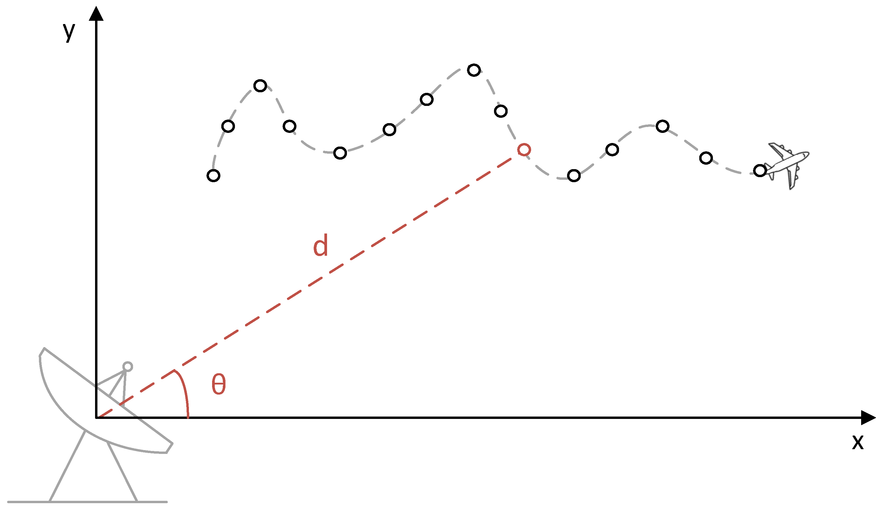
Figure 2.
The overall structure of our MIENet. It includes two typical models to achieve highly maneuvering target tracking. The input data is first processed by low pass filters to obtain auxiliary supervised signals (). Then auxiliary supervised signals and observations are fed into fusion denoising model. Afterward the denoised data is fed into the parameter estimation model to estimate the key turn rate of . Subsequently, the input observations and the estimated are all provided to UKF for estimating target states.
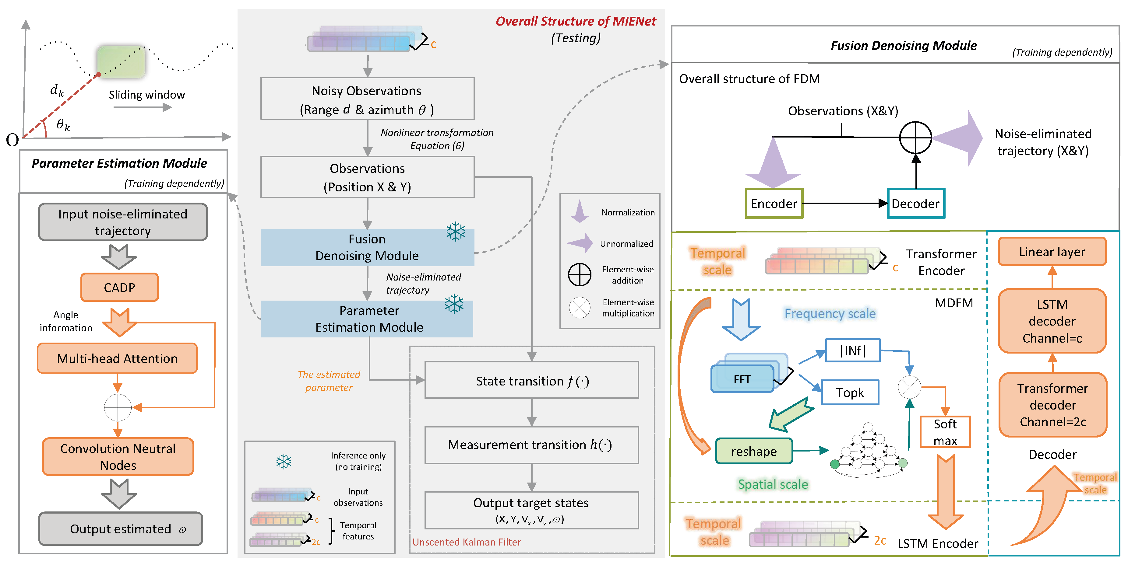
Figure 3.
The detailed structure of the fusion denoising model (FDM).
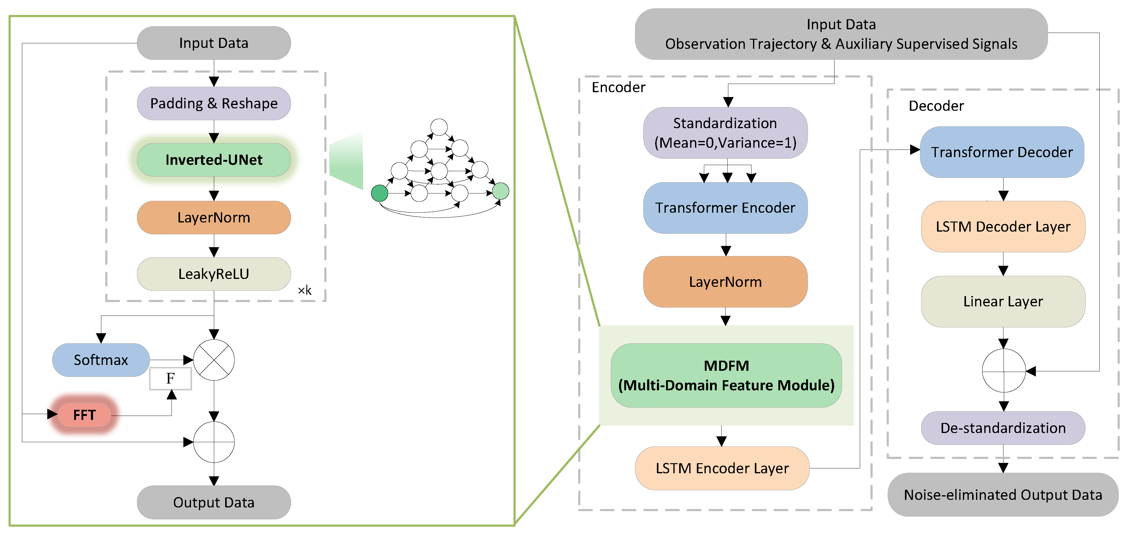
Figure 4.
The detailed structure of different UNet.
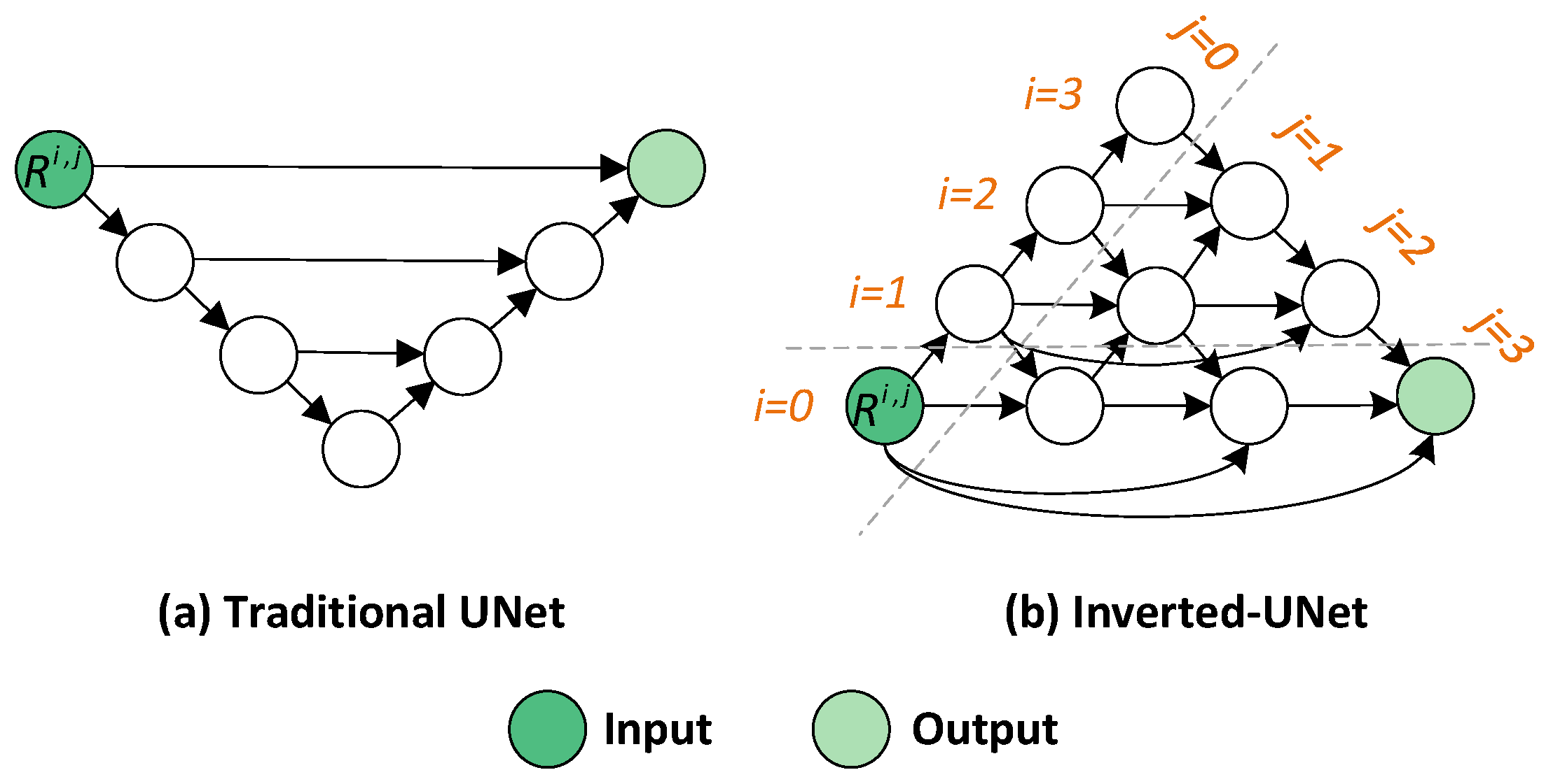
Figure 5.
The detailed structure of the parameter estimation model (PEM).

Figure 6.
Mean RMSEs of distance and velocity for four test trajectories.
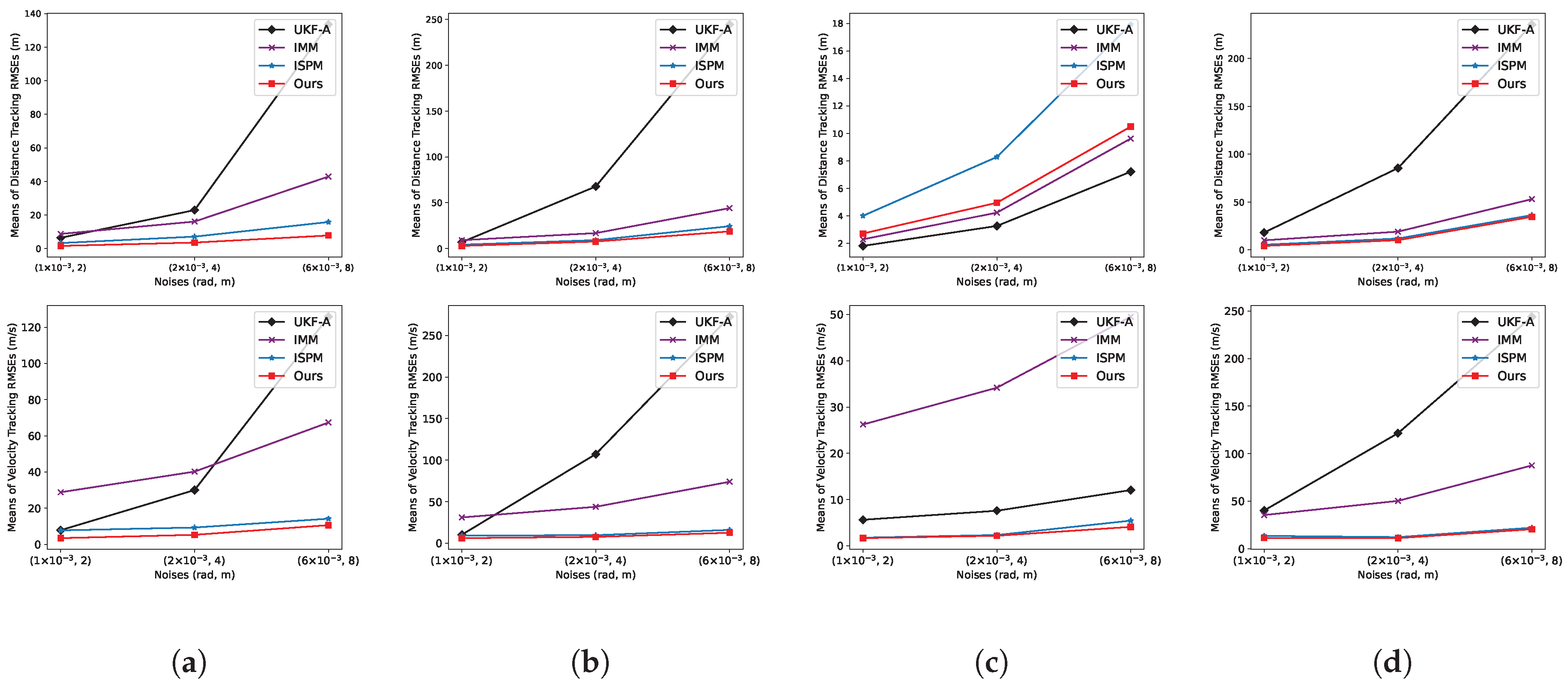
Figure 9.
Tracking trajectory results of our method on the SV248S dataset.


Table 1.
Parameter settings for the LAST datasets.
| Contents | Ranges |
|---|---|
| Initial distance from radar | [1 km, 10 km] |
| Initial velocity of targets | [100, 200m/s] |
| Initial distance azimuth | [-180°, 180°] |
| Initial velocity azimuth | [-180°, 180°] |
| Maneuvering turn rate | [-90°/s, 90°/s] |
| Variance of accelerated velocity noise | 10(m/s)2 |
Table 2.
Parameter settings for tracking test trajectories.
| Trajectories | Initial state | The first part | The second Part | The third part |
|---|---|---|---|---|
| 1 | [1000m, -18000m, 150m/s, 200m/s] | 27.4s, =50°/s | 52.6s, =40°/s | 27.4s, =30°/s |
| 2 | [1000m, -18000m, 150m/s, 200m/s] | 40s, =-30°/s | 27.4s, =70°/s | 40s, =50°/s |
| 3 | [500m, 2000m, -300m/s, 200m/s] | 25s, =60°/s | 42.4s, =50°/s | 40s, =-20°/s |
| 4 | [-20000m, -5000m, 250m/s, 180m/s] | 30s, =-30°/s | 17.4s, =70°/s | 20.9s, =-10°/s |
Table 3.
Means RMSEs of observation position and velocity for trajectories with UKF-A, IMM, ISPM and MIENet.
Table 3.
Means RMSEs of observation position and velocity for trajectories with UKF-A, IMM, ISPM and MIENet.
| Trajectories p(m) / v(m/s) |
Noise standard deviation (azimuth, range) |
UKF-A [61] | IMM [19] | ISPM [12] | MIENet (ours) | |
|---|---|---|---|---|---|---|
| 1 | (1×rad, 2m) | Part 1 Part 2 Part 3 |
6.667/11.38 6.329/7.463 6.457/7.963 |
9.193/32.57 8.689/28.72 8.366/25.87 |
3.770/7.920 3.370/8.030 2.490/7.040 |
1.800/4.170 1.500/3.100 1.350/3.100 |
| All | 6.420/7.860 | 8.720/28.84 | 3.280/7.770 | 1.580/3.470 | ||
| (2×rad, 4m) | Part 1 Part 2 Part 3 |
39.73/64.94 13.23/13.67 10.86/10.17 |
17.01/47.30 15.92/39.23 15.52/36.66 |
7.950/9.570 7.360/9.630 5.500/8.410 |
4.650/6.150 2.650/4.380 3.310/4.870 |
|
| All | 22.90/30.05 | 16.07/40.23 | 7.110/9.330 | 3.570/5.300 | ||
| (6×rad, 8m) | Part 1 Part 2 Part 3 |
139.2/208.9 136.4/124.3 132.7/109.7 |
62.80/147.8 41.62/63.69 40.46/60.04 |
17.80/13.59 15.88/14.67 13.26/13.83 |
9.170/10.15 7.250/12.20 4.520/8.590 |
|
| All | 133.5/125.8 | 42.90/67.37 | 15.80/14.21 | 7.780/10.64 | ||
| 2 | (1×rad, 2m) | Part 1 Part 2 Part 3 |
6.854/8.294 10.10/26.66 6.494/8.489 |
9.481/33.15 8.692/29.30 9.013/30.38 |
2.640/7.170 5.560/12.70 4.350/8.570 |
1.790/4.930 3.340/9.200 3.870/7.260 |
| All | 6.920/10.36 | 9.090/31.10 | 4.170/9.290 | 2.840/6.190 | ||
| (2×rad, 4m) | Part 1 Part 2 Part 3 |
12.04/12.22 94.06/172.2 83.27/118.6 |
17.95/45.88 15.82/44.09 16.33/42.03 |
5.600/8.870 11.74/10.53 9.970/10.07 |
3.440/6.190 10.06/9.740 11.53/10.58 |
|
| All | 67.66/107.1 | 16.78/43.87 | 9.110/9.750 | 7.600/7.690 | ||
| (6×rad, 8m) | Part 1 Part 2 Part 3 |
121.2/127.0 223.4/293.5 275.9/301.5 |
54.83/96.77 39.80/76.48 41.08/67.76 |
11.62/11.72 28.47/17.84 35.27/20.49 |
6.540/7.930 17.26/15.48 32.28/17.27 |
|
| All | 244.4/272.4 | 44.05/73.98 | 24.30/16.07 | 18.65/12.64 | ||
| 3 | (1×rad, 2m) | Part 1 Part 2 Part 3 |
1.651/5.706 1.561/5.125 2.214/6.587 |
2.106/24.70 2.010/25.08 2.723/28.50 |
5.030/1.810 4.590/1.650 2.320/1.870 |
3.300/1.920 2.590/1.550 3.120/1.760 |
| All | 1.810/5.640 | 2.290/26.23 | 4.000/1.770 | 2.710/1.670 | ||
| (2×rad, 4m) | Part 1 Part 2 Part 3 |
2.953/8.071 2.758/6.747 4.097/9.735 |
3.882/32.96 3.730/32.38 5.018/36.97 |
10.31/2.440 9.540/2.150 4.760/2.470 |
6.400/2.670 5.690/2.270 4.090/1.770 |
|
| All | 3.260/7.590 | 4.230/34.19 | 8.280/2.340 | 4.950/2.180 | ||
| (6×rad, 8m) | Part 1 Part 2 Part 3 |
6.277/14.22 5.747/10.03 9.921/18.34 |
8.626/50.51 8.169/46.74 11.79/52.27 |
22.15/5.630 21.03/3.200 9.160/7.020 |
14.98/5.070 10.43/4.040 8.120/3.980 |
|
| All | 7.210/12.06 | 9.620/49.53 | 17.92/5.450 | 10.49/4.100 | ||
| 4 | (1×rad, 2m) | Part 1 Part 2 Part 3 |
8.420/16.20 15.38/43.98 42.29/77.72 |
10.47/39.53 9.549/33.30 9.838/31.73 |
3.530/9.050 8.440/19.11 4.650/13.54 |
3.650/9.910 6.380/17.36 1.300/3.490 |
| All | 18.13/40.22 | 10.01/35.40 | 5.430/13.49 | 4.180/11.38 | ||
| (2×rad, 4m) | Part 1 Part 2 Part 3 |
28.23/43.75 99.56/175.2 114.5/124.9 |
20.41/55.48 17.93/50.32 18.37/44.73 |
7.150/11.13 18.42/13.35 10.81/12.76 |
8.440/6.140 16.01/18.94 2.370/6.230 |
|
| All | 85.48/121.5 | 19.06/50.31 | 11.89/12.21 | 10.16/11.14 | ||
| (6×rad, 8m) | Part 1 Part 2 Part 3 |
159.9/195.7 301.7/361.7 207.8/114.6 |
72.75/154.2 43.35/85.78 49.05/72.03 |
25.64/14.89 53.94/31.10 34.12/23.23 |
24.62/9.770 57.04/33.48 12.61/16.75 |
|
| All | 235.5/244.0 | 53.04/87.63 | 36.33/22.10 | 34.57/20.50 |
Table 4.
Category-Wise and Difficulty-Wise PR and SR Evaluations on SV248S.
| Category-Wise Evaluations | Difficulty-Wise Evaluations | |||||||||||||
|---|---|---|---|---|---|---|---|---|---|---|---|---|---|---|
| Vehicle | L-Vehicle | Airplane | Ship | Simple | Normal | Hard | ||||||||
| Trackers | PR | SR | PR | SR | PR | SR | PR | SR | PR | SR | PR | SR | PR | SR |
| STAR [62] | 0.7542 | 0.4911 | 0.8739 | 0.6555 | 0.8399 | 0.7517 | 1.0000 | 0.7562 | 0.8800 | 0.6228 | 0.7138 | 0.4653 | 0.6652 | 0.4177 |
| Ours | 0.7550 | 0.4944 | 0.8744 | 0.6598 | 0.8399 | 0.7530 | 1.0000 | 0.7611 | 0.8816 | 0.6278 | 0.7138 | 0.4675 | 0.6760 | 0.4440 |
Table 5.
Attribute-wise PR/SR evaluations on SV248S.
| Trackers | STO | LTO | DS | IV | BCH | SM | ND | CO | BCL | IPR |
|---|---|---|---|---|---|---|---|---|---|---|
| STAR [62] | 0.676/0.444 | 0.472/0.301 | 0.731/0.489 | 0.692/0.446 | 0.796/0.534 | 0.700/ 0.462 | 0.752/0.489 | 0.700/0.444 | 0.730/0.458 | 0.697/0.464 |
| Ours | 0.676/ 0.447 | 0.473/0.302 | 0.731/0.492 | 0.693/0.449 | 0.797/0.538 | 0.700/0.461 | 0.753/ 0.490 | 0.700/ 0.447 | 0.730/ 0.460 | 0.697/ 0.466 |
Table 6.
The adaptation and generalization of FDM ablation study (Gaussian-injected Noise).
| Methods RMSE(m) |
Gaussian-injected Noise (rad, m) |
||
|---|---|---|---|
| (2, 4) | (8, 10) | (11,13) | |
| Original Observation | 35.310 | 140.94 | 193.77 |
| Butterworth Filter | 28.000 | 112.09 | 153.65 |
| ISPM-NEN [12] | 17.359 | 61.978 | 84.804 |
| FDM (ours) |
13.593 (↓61.5%) |
43.690 (↓69.0%) |
61.135 (↓68.4%) |
Table 7.
The adaptation and generalization of FDM ablation study (Uniform-injected Noise).
| Methods RMSE(m) |
Uniform-injected Noise (rad, m) |
||
|---|---|---|---|
| (12, 21.3) | (40.3, 56.3) | (75, 133.3) | |
| Original Observation | 61.536 | 112.78 | 153.84 |
| Butterworth Filter | 47.836 | 87.673 | 119.59 |
| ISPM-NEN [12] | 28.994 | 52.348 | 71.290 |
| FDM (ours) |
23.295 (↓62.1%) |
40.333 (↓64.2%) |
54.277 (↓64.7%) |
Table 8.
MDFM to FDM ablation study.
| Methods RMSE(m) |
Noise | ||||
|---|---|---|---|---|---|
| (2 × rad, 4m) | (8 × rad, 10m) | (11 × rad, 13m) | |||
| FDM w/o MDFM |
pos(m) | Part 1 Part 2 Part 3 |
15.53 16.34 15.69 |
49.34 42.67 44.04 |
74.20 58.67 62.43 |
| All | 15.97 (↓36.3%) |
44.81 (↓55.2%) |
63.91 (↓53.5%) |
||
| Ours | pos(m) | Part 1 Part 2 Part 3 |
11.63 10.25 9.96 |
39.28 33.58 38.76 |
55.11 46.97 57.77 |
| All | 10.55 (↓57.9%) |
36.45 (↓63.5%) |
52.02 (↓62.1%) |
||
Table 9.
Results of the ablation study.
| Tracking variations |
MDFM | MHN | PCLoss | Distance (m) / Velocity (m/s) |
|---|---|---|---|---|
| Ablation 1 | ✓ | ✓ | 15.83 / 29.61 | |
| Ablation 2 | ✓ | ✓ | 16.90 / 14.07 | |
| Ablation 3 | ✓ | ✓ | 9.900 / 13.55 | |
| Ours | ✓ | ✓ | ✓ | 7.780 / 10.64 |
Disclaimer/Publisher’s Note: The statements, opinions and data contained in all publications are solely those of the individual author(s) and contributor(s) and not of MDPI and/or the editor(s). MDPI and/or the editor(s) disclaim responsibility for any injury to people or property resulting from any ideas, methods, instructions or products referred to in the content. |
© 2025 by the authors. Licensee MDPI, Basel, Switzerland. This article is an open access article distributed under the terms and conditions of the Creative Commons Attribution (CC BY) license (http://creativecommons.org/licenses/by/4.0/).
Copyright: This open access article is published under a Creative Commons CC BY 4.0 license, which permit the free download, distribution, and reuse, provided that the author and preprint are cited in any reuse.


