Submitted:
29 August 2024
Posted:
30 August 2024
You are already at the latest version
Abstract
Unmanned Aerial Vehicles (UAVs) have become increasingly important in various applications, including environmental monitoring, disaster response, and surveillance, due to their flexibility, efficiency, and ability to access hard-to-reach areas. Effective path planning for multiple UAVs exploring a target area is crucial for maximizing coverage and operational efficiency. This study presents a novel approach to optimizing collaborative navigation for UAVs using Multi-Agent Reinforcement Learning (MARL). To enhance the efficiency of this process, we introduce the Adaptive Dimensionality Reduction (ADR) framework, which includes Autoencoders (AEs) and Principal Component Analysis (PCA) for dimensionality reduction and feature extraction. The ADR framework significantly reduces computational complexity by simplifying high-dimensional state spaces while preserving crucial information. Additionally, we incorporate communication modules to facilitate inter-UAV coordination, further improving path planning efficiency. Our experimental results demonstrate that the proposed approach significantly enhances exploration performance and reduces computational complexity, showcasing the potential of combining MARL with ADR techniques for advanced UAV navigation in complex environments.
Keywords:
Multi-Agent Reinforcement Learning (MARL)
; Dimensionality Reduction
; Unmanned Aerial Vehicles (UAVs)
1. Introduction
Unmanned Aerial Vehicle (UAV) technology has made tremendous progress in recent years, with an increasingly wide range of applications, from military reconnaissance [1] to logistics [2] and distribution, and from agriculture and plant protection [3] to disaster relief [4]. The development of UAV technology has provided efficient and economical solutions [5] for these industries. UAVs are popular for monitoring complex terrain due to their high flexibility, mobility, and low deployment costs. [6] Simultaneously, utilizing multiple UAVs to explore target areas and establish a communication system for information sharing can significantly enhance exploration efficiency, reduce overall costs, and minimize the impact of individual UAV failures on terrain exploration. However, limited resources make informative path planning (IPP) a critical issue.
IPP methods include grid-based search, potential field methods, and heuristic algorithms like A* [17]. Grid-based search ensures thorough coverage by dividing the area into a grid and systematically exploring each cell, but it is computationally expensive and inefficient for large areas. Potential field methods create a virtual field where UAVs are attracted to the target and repelled by obstacles, resulting in smooth paths; however, they can become trapped in local minima. Heuristic algorithms such as A* provide optimal paths by evaluating multiple potential routes and selecting the best one based on cost. Still, they struggle with dynamic and complex scenarios where environmental conditions constantly change.
Reinforcement Learning (RL) [7] has emerged as a promising solution to address these limitations. RL enables UAVs to learn and adapt to dynamic environments by interacting with the environment and receiving feedback on their actions. This learning process allows the development of optimal policies that improve over time, providing robust solutions to complex scenarios. However, traditional RL methods are primarily designed for single-agent systems and face significant challenges when extended to multi-agent scenarios, such as scalability and coordination among agents.
To overcome these challenges, Multi-Agent Reinforcement Learning (MARL) has been developed [8,16], which extends RL to multiple interacting agents. MARL enables UAVs to handle dynamic and uncertain environments collaboratively by learning and adapting through interaction with the environment and each other. MARL allows for the development of optimal policies that improve over time and provide robust solutions to complex scenarios. This makes it particularly powerful in situations where traditional methods fall short. Additionally, MARL facilitates coordination among multiple UAVs, enhancing their collective performance. However, despite these advantages, MARL approaches can be computationally intensive and may suffer from efficiency and scalability issues when applied to large-scale multi-UAV systems.
In our method, images captured by the UAVs are first processed through a combination of Autoencoders (AEs) and Principal Component Analysis (PCA) as part of the Adaptive Dimensionality Reduction (ADR) framework. This preprocessing step significantly reduces the computational load by simplifying high-dimensional input data while preserving essential features. AEs are primarily used for feature extraction and handling complex data, while PCA provides an efficient means of further reducing the dimensionality, particularly in less complex scenarios. The output from the ADR framework is then fed into the actor network of the MARL framework, which is responsible for decision-making and path planning. Furthermore, we deploy communication modules that allow UAVs to share information and coordinate their actions effectively. This integrated approach not only enhances the overall efficiency of the system but also improves the performance and robustness of UAV navigation in complex and dynamic environments.
This paper focuses on active data collection using a team of UAVs for terrain monitoring scenarios. The objective is to create a map of an initially unknown, non-homogeneous binary target variable on a 2D terrain, such as identifying crop infestations in an agricultural setting or locating victims in a disaster scenario, utilizing image measurements captured by the UAVs. We address the challenge of multi-agent IPP, where we design information-rich paths for the UAVs to cooperatively gather sensor data while adhering to energy, time, or distance constraints. The goal is to enable the UAVs to dynamically monitor the terrain, concentrating on areas of interest with high information value.
The main contribution of this paper is the introduction of a novel multi-agent deep reinforcement learning-based IPP approach for adaptive terrain monitoring using UAV teams. Our approach supports decentralized on-board decision-making and achieves cooperative 3D path planning with variable team sizes. Our main contributions include:
1. Markov Modeling and Environment Modeling: We develop a comprehensive Markov model to represent the states of UAVS and the environment dynamics, enabling more accurate predictions and decision-making in complex terrains.
2. ADR framework: We introduce the ADR framework, which integrates AEs and PCA to preprocess image data captured by the UAVs. This dual-method approach allows for efficient dimensionality reduction and feature extraction, enhancing computational efficiency and improving the quality of the input for the reinforcement learning framework.
3. Implementation of Communication Modules: We establish robust communication protocols that allow UAVs to share information and coordinate their actions effectively. This enhances overall system performance, ensuring better coverage and data collection.
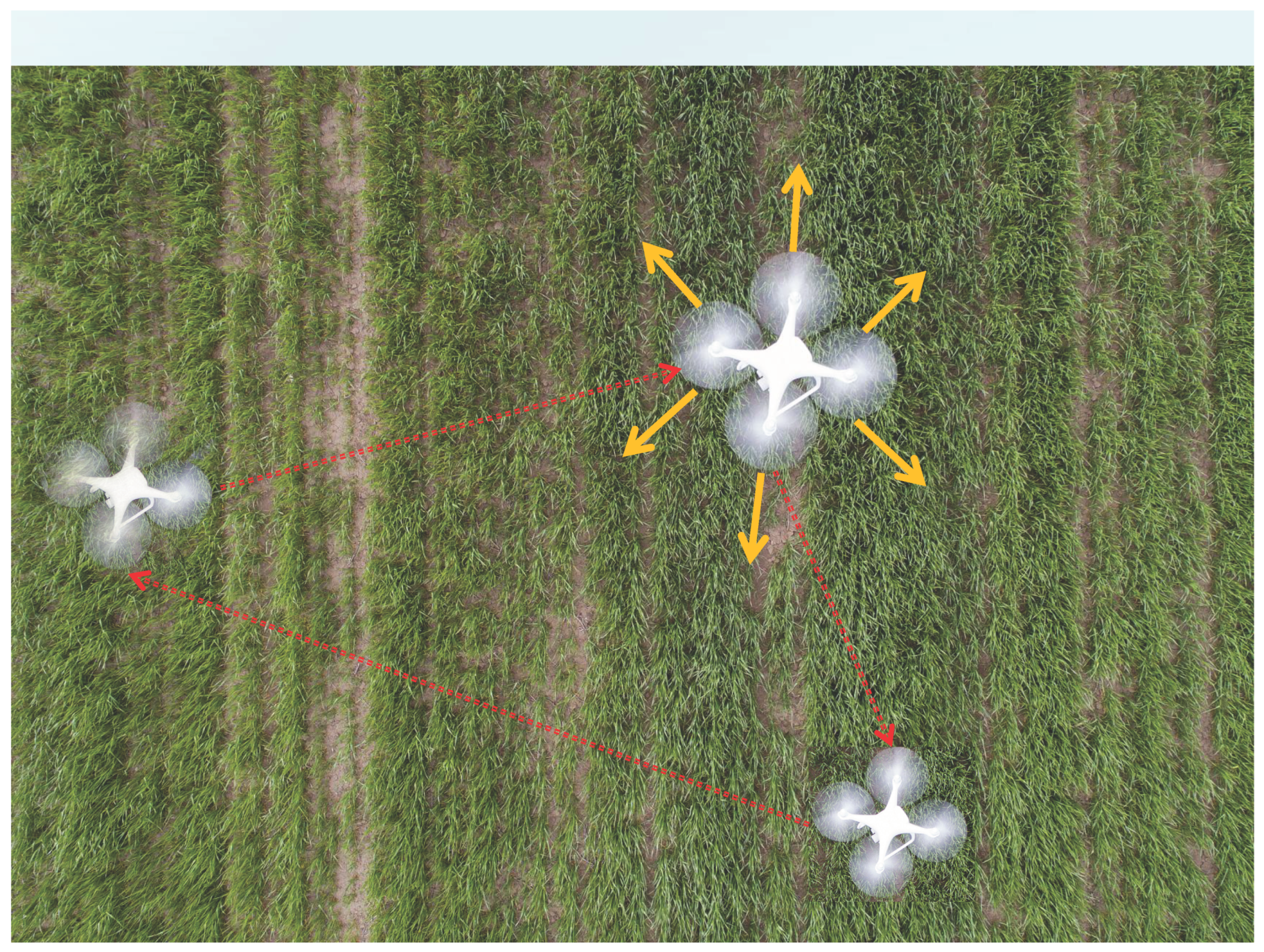
Figure 1.
This figure illustrates a multi-UAV (Unmanned Aerial Vehicle) system operating cooperatively above a crop field. Three UAVs are shown flying over the crops. The red dashed arrows indicate the communication paths between the UAVs. Each UAV determines its next measurement location based on locally available information, as indicated by the yellow arrows showing possible action directions. This cooperative path planning enables the UAVs to effectively cover and monitor temperature variations or other parameters of interest in the field. In the figure, the size of the drones represents the different altitudes at which they fly.
Additionally, we address the credit assignment problem in cooperative IPP using counterfactual multi-agent policy gradients (COMA). Our approach significantly improves planning performance and computational efficiency, demonstrating its potential for UAV navigation in complex and dynamic environments.
2. Related Work
Traditional UAV IPP methods include the grid-based search proposed by Yamauchi [9] (1997), the potential field methods introduced by Khatib (1986) [10], and heuristic algorithms like A* developed by Hart, Nilsson, and Raphael (1968) [11]. Grid-based search ensures thorough coverage but is computationally expensive and inefficient for large areas. Potential field methods create smooth paths using virtual forces but often get trapped in local minima. The A* algorithm selects optimal paths by evaluating multiple potential routes but struggles in dynamic and complex scenarios. To address these limitations, LaValle (1998) [12] proposed the Rapidly-exploring Random Trees (RRT) algorithm, which efficiently explores large spaces but often produces non-smooth paths. The Particle Swarm Optimization (PSO) method, introduced by Kennedy and Eberhart (1995) [13], optimizes flight paths through iterative improvement but requires careful parameter tuning and is computationally intensive. The limitations of these traditional methods highlight the need for more advanced solutions, such as RL, to achieve more effective UAV path planning in dynamic and complex environments.
RL has also been widely applied to UAVs. Wei et al. [14] designed a constrained exploration and exploitation strategy using Q-networks, but this method is limited to single-agent intelligence. Vashisth et al. [15] proposed a dynamically constructed graph restricting agents to local planning actions, allowing for better path exploration. However, it cannot transfer policies to real robots without localization and perception uncertainties. Rueckin et al. [16] combined tree search with an offline-trained neural network, significantly improving information perception capabilities with small data sets. Pirinen et al. [17] introduced a strategy for using UAVs to find unknown target regions based on limited visual cues. Chen et al. [18] developed a graph-based deep RL method for exploration, selecting map frontiers that reduce map uncertainty and travel time. However, their approach is limited to 2D workspaces, whereas we consider 3D planning. Jonas Westheimer et al. [19] introduce new network feature representations to effectively learn path planning in a 3D workspace. However, their research faces significant efficiency issues as the amount of data increases.
MARL is a more promising direction for IPP as it is closer to real-world scenarios and introduces more complex environments and higher requirements. Foerster et al. [20] (2018) introduced counterfactual COMA to address the credit assignment problem. Lowe et al. [21] (2017) proposed the Multi-Agent Deep Deterministic Policy Gradient (MADDPG), which allows for centralized training and decentralized execution, improving performance in complex environments. Yousef et al. [22] proposed a novel mean-field flight resource allocation optimization method to minimize the Age of Information (AoI) of perceived data. This method successfully optimized the UAV flight trajectories and the data collection scheduling of ground sensors, showing significant improvements compared to DQN. Iqbal and Sha (2019) [23] proposed Independent Q-Learning (IQL), which simplifies the training process of multiple agents while maintaining high performance. However, the computational complexity and scalability issues of MARL in large-scale systems still require further research and solutions. To address this, recent studies such as Zhang et al. [24](2021) have proposed a hierarchical MARL method to reduce computational burden and improve scalability through hierarchical decision-making. Additionally, Peng et al. [25](2022) introduced a distributed MARL framework that reduces communication overhead and enhances system resilience, demonstrating potential applications in large-scale multi-agent systems.
In order to improve the training effect of the network, David et al. (1986) [26] proposed the autoencoder (AE) based on the back propagation of neuron-like unit networks. Hinton et al. (2006) [27] first proposed the use of gradient descent to fine-tune the weights of AE networks, reducing the data dimension to improve the training effect. Although AE can effectively solve the problem of insufficient feature extraction and overfitting, there are also some problems, such as long training time and insufficient accuracy. In order to solve these problems, scholars have conducted research and made some improvements to AE.
For image processing, the working principle of AE requires the data to be transformed into a one-dimensional vector for post-processing, which will lead to the loss of two-dimensional structure information of the image. Therefore, Ranjan et al. [28] introduced convolutional neural networks to preserve two-dimensional spatial information by replacing the fully connected layers with convolution and pooling operations in them. Zhao et al. [29] proposed image classification based on DSAE dimensionality reduction, but it will cause the problem of gradient disappearance as the number of convolutional neural network (CNN) layers increases. To this end, they added a residual network module to the 3D CNN and proposed 3DDRN [30]. For samples of various sizes, DSAE can effectively extract low-dimensional features from the original image and perform well in classification. Guo et al. [31] performed feature extraction by adding a CNN to a stacked autoencoder (SAE). This method can achieve high accuracy through simple unsupervised pre-training and single supervised training, simplifying the complex calculation process. For the noise in the image, Revathi et al. [32] proposed an AE method based on DCNN to deal with the noise in the image, which effectively improved the accuracy.
To further exploit the potential of AE, Cheng et al. [33] added a regularization term to the hidden neurons of a discriminative stacked autoencoder (DSAE) to bring similar samples closer together in the mapping space. At the same time, this approach can use the regularization optimization objective function to fine-tune the DSAE. Inspired by them, Wang et al. [34] conducted a study on the relationship between the number of neurons in the hidden layer and classification accuracy and proposed that for simple images [35], the gain is no longer obvious after the number of neurons is close to the input data dimension. However, for complex image processing, the classification progress will improve as the number of neurons increases.
PCA is another linear feature projection method used to reduce the dimensionality of the data. It simplifies the classifier design and reduces the computational burden of pattern recognition technology by reducing the dimension and keeping most of the relevant features in the distant data. Qifa et al. [36] pointed out that the traditional singular value decomposition (SVD) is not well applicable when there are outliers and missing data in the measurement. They leveraged the sensitivity of PCA to outliers and applied iterated reweighted least squares (IRLS) to decompose each element, leading to the development of their L1-PCA approach. Chris et al. [37] used PCA to minimize the sum of squared errors and proposed rotation invariant L1-norm PCA (R1-PCA). This method guarantees that there is a unique global solution and the solution is rotation invariant. After comparison, R1-PCA can deal with outliers more effectively, and when extended to K-means clustering, L1-norm K-means performs worse, while R1 K-means method is significantly better. However, PCA can only describe a good coordinate system for all feature distributions and does not consider class separation. Therefore, in order to improve the accuracy of recognition, it is necessary to provide high-level separable features. Matsumura et al. [38] used PCA technology to analyze EMG data, which effectively improved the recognition accuracy and recognition speed.
To further enhance the efficiency of MARL in UAV path planning, we propose an innovative approach incorporating ADR. By preprocessing the image data captured by the UAVs, the ADR performs dimensionality reduction and feature extraction, significantly reducing the computational burden of high-dimensional input data. The output from the autoencoders is then fed into the execution network of the MARL framework, thereby improving the overall system efficiency and performance and enhancing the robustness of UAV navigation in complex and dynamic environments.
3. Method
3.1. Markov Decision Process Modelling
To address the problem of optimizing UAV collaborative navigation in multi-agent reinforcement learning, we model it as a Markov Decision Process (MDP). The MDP process, as illustrated in Figure 2, serves as a mathematical framework to model decision-making in scenarios where outcomes are influenced by both random factors and the decisions made by an agent. An MDP can be described by the tuple (S, A, R, , T). The meaning of each element is explained below.
S represents the state space, encompassing all possible states where an agent can exist. Here, we mainly consider the state of the map. We take a picture of the measurement range through the camera of the UAV and obtain the likelihood estimate of UAV i projected onto the flat terrain at time t. Each UAV i stores a local posterior map confidence . According to the measurement value of UAV i and the altitude value, its position can be obtained. We define as the state of the global environment at time t, where represents the current location, and b represents the remaining mission budget.
A denotes the action space, comprising all possible actions an agent can take to influence the environment. Each agent takes an action of a fixed step size in a 3D discrete environment, which includes east, south, west, north, up, and down. They can only move within a prescribed discrete location grid P and cannot move outside the environment.
R is the reward function, mapping state-action pairs to real numbers and providing feedback to the agent by assigning a numerical reward for each action taken in a given state. Our reward function is expressed in Equation 1:
where represents the joint action constituted by all UAV actions, and represents the state of the map at time t. From this, we can see that the entropy reduction of the weighted map from the current state to the next state will be rewarded accordingly, because a reduction in entropy signifies a decrease in environmental uncertainty, indicating that the UAVs have successfully gathered more valuable information, thereby effectively improving the quality of task completion. In the reward function, the parameter controls the weight of the entropy reduction term, thereby influencing the emphasis on reducing environmental uncertainty and can be flexibly adjusted according to the situation. The parameter , as a bias term, can adjust the baseline reward to encourage or discourage specific behaviours, such as promoting more frequent exploration of new areas by the UAVs or maintaining specific flight paths.
is the discount factor, a value between 0 and 1, that determines the importance of future rewards, balancing short-term and long-term gains.
T represents the transition model, which describes the probability of moving from one state to another given a specific action, thereby capturing the dynamics of the environment and its inherent uncertainties.
We generally use to represent a strategy, where Equation 2 is a probability function that represents the probability of taking action a in state s.
The policy can be divided into deterministic policy and stochastic policy. The former only outputs one definite action for each state; that is, only this action has a probability of 1, and all other actions are 0. The latter outputs a probability distribution over the actions, from which sampling can obtain an action.
The value function of the MDP is related to the policy, and different policies will produce different actions and states and obtain different rewards. The expected reward of a state based on policy in an MDP is called the state value of . All the state values constitute the state value function . Similarly, the expected reward of state taking action a and executing based on policy is called action-value, which constitutes action-value function . The relationship between the two value functions can be expressed by Equation 3.
The policy that gives the agent the most expected reward is the optimal policy. There may be many optimal policies, but they all have the same state-value function. We can also obtain the optimal action-value function. The optimal state value function is obtained to find the optimal policy to obtain the maximum expected reward, and the goal of reinforcement learning is completed.
3.2. Multi-Agent Reinforcement Learning
A single RL agent acquires knowledge through interactions with the external environment. Specifically, the agent responds to its surroundings by taking actions based on its policy and the conditions at the time. In return, the agent receives a reward value that offers feedback on the effectiveness of its actions. Unlike supervised learning, the primary objective of reinforcement learning is to learn a policy that maximizes rewards—often a delayed goal.
Most successful applications of RL are in single-agent scenarios where there is no need to model or predict other agents in the environment. However, many important application scenarios involve interactions among multiple agents, making the problem more complex. For example, multiple robots working together, multiplayer games, etc., are all multi-agent scenarios. Additionally, multi-agent self-play is an effective RL method. Therefore, extending RL from single-agent to multi-agent environments is crucial for designing intelligent systems capable of interacting with humans or other agents.
From the above descriptions, it’s evident that while the application of RL in single-agent scenarios is relatively straightforward, as there is no need to consider the behaviours of other agents, the situation becomes significantly more complex in multi-agent scenarios. In these environments, each agent must learn how to interact with the environment and cooperate with or compete with other agents. These challenges in multi-agent environments have driven researchers to develop more sophisticated algorithms and models.
One significant algorithm in this context is COMA. COMA is a policy gradient method designed for multi-agent reinforcement learning to address coordination issues among multiple agents. The structure of COMA, as illustrated in Figure 3, introduces a counterfactual baseline based on the joint action-value function, which reduces variance and improves the efficiency and stability of policy gradient estimates. This approach enables better coordination among multiple agents and performs better in complex multi-agent environments.
For agent a, let denote its action, and represent its trajectory of observations and actions. Let denote the joint actions of all agents, the joint actions of all other agents except a, and s the global state of the system. The counterfactual baseline for an agent (a) can be calculated as Equation 4.
The second term on the right-hand side is essentially the expectation of Q over all possible actions of agent a while keeping the actions of other agents fixed. You can see that this form is similar to the way the advantage function is calculated in single-agent RL with AC or A2C as Equation 5:
where
The distinction is found in Equation 4, which calculates to provide a more detailed evaluation of the policy of each agent, distinguishing the contribution of individual policies to the overall strategy.
With the objective function defined, the next step is to compute the gradient and update the policy. The policy gradient for COMA is given by Equation 7
In Equation (2), k denotes the iteration number, and represents the parameters at iteration k. For the derivation and proof of this result, please refer to the literature [20].
Additionally, the update of is performed using the TD() method, and target network parameters are periodically updated to compute the target value.
3.3. AE and PCA
An autoencoder is an effective encoding method used for learning and extracting the main features of data. Implemented in neural networks, autoencoders are used to reconstruct the input information. As the training process of autoencoders does not require data labels, they are considered an unsupervised learning model and method. The structure of autoencoders generally shown in Figure 4 includes two parts:
Encoder
It learns the main features of the input data (dimensionality reduction) and transfers the input signal to another space to represent it in a different form, as described in Equation 8.
where is the weight matrix between the input and hidden layers, and is the bias vector. is a non-linear activation function.
Decoder
It transforms the signal from the latent space back to the original space and reconstructs the input data, as described in Equation 9.
where is the weight matrix between the hidden and output layers, and is the bias vector. is a non-linear activation function, which can be a sigmoid or tanh function.
The encoding process can be considered mapping the input data X to a specific coding h in the latent space. In contrast, the decoding process reconstructs the data from the latent space back to the original space. The AE training minimizes the difference between the input and reconstructed data. The commonly used loss functions include mean squared error (MSE) (as shown in Equations 10 and 11) and cross-entropy loss (as shown in Equations 12 and 13).
The MSE loss is defined as:
The cross-entropy loss is defined as:
From the perspective of the loss function, it does not have labels, distinguishing it from traditional autoencoders trained through unsupervised methods. The decoding process separates the parameters of the encoder and decoder. simplifies the training, reducing the number of training parameters by half. This is called the tied weights autoencoder (TAE). For loss optimization, stochastic gradient descent (SGD) can be used. Unlike PCA, which updates batch-by-batch, autoencoders update more flexibly. Generally, a regularization term (also known as weight decay) is added to the loss function to control and reduce the degree of model overfitting. The regularization parameter controls the strength of the regularization and ranges from 0 to 1, as shown in the Equation 14:
Unsupervised Adversarial Erasing (UAE) and ordinary autoencoders (AE) differ significantly in principle and structure. An ordinary autoencoder (AE) encodes input data x into a lower-dimensional representation z (encoder: ), and then reconstructs the input data from z (decoder: ), aiming to minimize the reconstruction error . In contrast, UAE generates adversarial samples by partially erasing or modifying the input image x, aiming to teach the model to learn more robust and generalizable features. The objective function of UAE includes an adversarial loss term, typically expressed as Equation 15:
where G is the generator and D is the discriminator. Through this adversarial training, UAE ensures that the model maintains high performance even when parts of the image are occluded or erased, rather than merely reconstructing the input data.
UAE provides several advantages, including enhanced robustness, improved generalization, and an emphasis on key features through adversarial training. By partially erasing or modifying input images, UAE trains models to be more resilient to noise and occlusions, enabling them to learn more representative features and maintain high performance even under challenging conditions. We will use UAE to process images, aiming to improve model robustness and generalization by focusing on critical features and ensuring consistent performance despite partial occlusions or modifications.
In this study, we employed PCA for dimensionality reduction to enhance computational efficiency and accelerate strategy convergence in multi-agent reinforcement learning. PCA operates by applying a linear transformation to map high-dimensional data into a new, lower-dimensional space, thereby retaining the essential information while reducing redundancy.
We began by standardizing the input data, ensuring that each feature had a mean of 0 and a standard deviation of 1, which eliminates the influence of different feature scales. Next, we computed the covariance matrix of the standardized data, defined as Equation 16:
where X represents the data matrix.
Following this, we performed an eigenvalue decomposition on the covariance matrix to obtain a set of eigenvalues and their corresponding eigenvectors. These eigenvectors represent the principal directions in the new space, with the eigenvalues indicating the variance along these directions. We then sorted the eigenvalues in descending order and selected the top k eigenvectors to form the basis vectors for the new lower-dimensional space, represented by the matrix W.
Finally, we projected the original data matrix X into this lower-dimensional space, yielding the reduced data matrix, shown as Equation 17:
This process allowed us to significantly reduce the dimensionality of the data while preserving its key characteristics, thus enhancing the efficiency of multi-agent reinforcement learning and speeding up the model training process.
3.4. The Proposed Work
3.4.1. Network Setting
This section discusses the design of neural network representations for actor and critic networks using COMA (Counterfactual Multi-Agent) in 3D robotic applications, and the overall network architecture will be presented in Figure 5.
Actor-Network: The actor network is represented by a neural network parameterized by , conditioned on the agent i and its local state . Input features include the agent identifier i, remaining mission budget b, and the following spatial inputs: (a) a position map centered around the position of the agent, encoding the boundaries and the communicated positions of other agents, where values represent agent altitudes.; (b) the local map state ; (c) the weighted entropy of the local map state ; (d) the weighted entropy of the measurement ; and (e) the map cells spanned by all agents’ fields of view within the communication range (’footprint map’). To handle terrain monitoring tasks, the network employs convolutional encoders and multi-layer perceptrons. The logits of the actor, , predict the stochastic policy through a bounded softmax function.
Critic Network: The critic network is represented by a neural network parameterized by , receiving the same input features (a-e) as the actor-network, as well as additional global information: (f) a global position map encoding all agent positions ; (g) the global map state ; (h) the weighted entropy of the global map state ; and (i) the map cells spanned by all agents’ fields of view. The critic network uses this information to learn the counterfactual baseline, outputting Q-values for each agent action . Inputs are provided at grid resolution , with the map resolution downsampled to , and scalar inputs i and b expanded to constant-valued 2D feature maps.
3.4.2. Communications Module
To enhance the efficiency of multi-agent reinforcement learning, we designed and implemented a communication module with a limited range, allowing UAVs to share their field-of-view information within a specified range, thereby achieving more efficient collaboration and task execution, the working process of the communication module will be presented in Figure 6. Each UAV is equipped with a communication module and an RGB camera sensor to capture image data representing the current state. This communication module includes:
1. Data Transmission Unit: Ensures low-latency and high-bandwidth data transmission while considering the communication range limitation.
2. Data Processing Unit: Receives and processes field-of-view data from other UAVs.
In the simulation environment, each UAV periodically transmits its map data and key observations to other UAVs within the communication range. The UAVs process the captured image data to extract current state information, including altitude, speed, and direction. Shared information includes:
1. Position and Status Information: The current position, speed, direction, and altitude of each UAV.
2. Environmental Observation Information: Map data collected from virtual sensors, including terrain, obstacles, and other environmental features.
Upon receiving the field-of-view information from other UAVs within the communication range, the data processing unit in the communication module performs data fusion. This process involves:
1. Data Alignment: Temporally and spatially aligning data based on timestamps and position information from different UAVs.
2. Information Integration: Combining the field-of-view data from multiple UAVs using a weighted average method to generate a comprehensive global environmental view.
The integrated data gives each UAV a global view of the environment, enhancing their situational awareness and enabling better decision-making. This global view includes detailed maps of the terrain, locations of obstacles, and the positions and statuses of other UAVs.
4. Experiment
To verify that drones can efficiently collaborate in different scenarios, we will conduct experiments in three distinct environments. These scenarios are as follows: Scenario 1 - a strip area occupying a certain percentage of the space, Scenario 2 - a rectangular area located in the corner of the scene, and Scenario 3 - a strip area in the middle. The images of scenarios 1, 2, and 3 will be respectively presented in Figure 7, Figure 8, and Figure 9. We identified real terrains matching these shapes and created heatmaps based on the areas of interest. In these heatmaps, the dark (especially red) parts are recognized as areas of high interest. During the mission, drones need to collect as much information as possible from these high-interest areas.
In our experiments, we focused on the training processes of AE and PCA separately, using large-scale image data of 493x493 pixels captured by UAVs to perform dimensionality reduction, thereby improving computational efficiency and reducing data complexity. For AE training, we used an encoder-decoder network to compress the input images into a 64-dimensional latent space, optimizing the process by minimizing the reconstruction loss between the input and reconstructed images. The AE was trained on 6000 images captured by the UAVs, with a batch size of 128, an initial learning rate of 0.001 using the Adam optimizer, and training was conducted over 100 epochs. This process successfully extracted key features from the images and significantly reduced the data dimensionality. On the other hand, PCA used Incremental Principal Component Analysis (IPCA) to process the same data, reducing it to 121 principal components. Given the large data volume, IPCA was applied with a batch size of 4096, using an incremental fitting approach to manage the computational demands of large-scale data processing. Each batch of data was flattened into a one-dimensional vector before being input into the IPCA model, and the dimensionality-reduced results were then converted into 11x11 tensors.
For each experiment, we execute 50 terrain monitoring missions in a 50-meter by 50-meter area with a map resolution of 10 centimetres. The planning resolution is set to 10 meters, and the flight altitude is limited between 20 meters and 30 meters. We use a camera with a 60-degree field of view, ensuring adjacent measurements do not overlap when taken from the lowest altitude. Considering increased sensor noise at higher altitudes, we simulate noise probabilities of 0.98, 0.75, and 0.625 for altitudes of 5, 10, and 15 meters, respectively. The UAV team consists of 4 agents with a communication radius of 25 meters.
The experimental environment includes a seed value of 3 to ensure varied start positions for each UAV. The sensor is an RGB camera with a resolution of 10 centimetres (57 pixels in both x and y directions). The simulation uses a random field with a cluster radius of 5 meters. The mapping prior is set to 0.5. The experiment includes constraints such as a spacing of 5 meters, a minimum altitude of 5 meters, a maximum altitude of 15 meters, and a budget of 14 actions. UAVs have a maximum speed of 5 meters per second, a maximum acceleration of 2 meters per second squared, and a sampling time of 2 seconds. Missions are conducted using the COMA method in training mode, with 1500 episodes and a patience of 100. The remaining relevant hyperparameters will be presented in Table 1.
In all experiments, we will primarily measure the performance of the algorithms using rewards, supplemented by Q-values and entropy to further evaluate the experimental outcomes. The reward value directly reflects the effectiveness of a strategy in completing tasks within a specific environment and serves as the core metric for evaluating the quality of the strategy. It clearly indicates whether the strategy meets the expected goals, which is particularly crucial in complex scenarios. The Q-value assesses the long-term value of the strategy, offering insights into future decisions; a high Q-value suggests that the strategy is effective not only in the current step but also in multiple future steps, which is essential for the long-term optimization of path planning. Entropy evaluates the stability and diversity of the strategy; low entropy indicates that the strategy is becoming stable, while high entropy may suggest that the strategy is still exploring different decision paths. By considering the reward, Q-value, and entropy together, a more comprehensive understanding of the overall performance of the algorithm can be achieved, ensuring more stable and efficient path planning in practical applications.
5. Result
5.1. Result in Scenario 1
In the multi-agent reinforcement learning task of Scenario 1, different dimensionality reduction strategies have a significant impact on model performance, and the reward trend will be presented in Figure 10. Overall, the AE strategy performed the best throughout the training process, ultimately achieving the highest reward value of approximately 0.35, demonstrating strong stability and learning effectiveness. At the beginning of training, the PCA (red line) method slightly outperforms both AE (blue line) and the method without dimensionality reduction (green line), suggesting that PCA has certain advantages in the initial exploration of strategies. However, the slightly fluctuating performance of AE may be attributed to the fact that the dimensionality reduction process introduces additional complexity, requiring more time to adapt to the environment.
While PCA performs better than AE and the non-reduced strategy during the first 200 training rounds, its performance becomes more erratic as training progresses, failing to maintain a consistent advantage. Consequently, the final reward value for PCA is slightly lower than that of AE, around 0.3. The strategy without dimensionality reduction performs the worst in the initial stages and exhibits slow growth, with a final reward value of only about 0.25. This outcome suggests that in complex scenarios, appropriate dimensionality reduction is crucial for enhancing the effectiveness of multi-agent reinforcement learning. Specifically, the AE method is more effective in capturing key features within the scene, thereby improving overall strategy effectiveness.
In the Q-value performance of Scenario 1, as shown in Figure 11, the PCA method (red line) performs the best in the later stages of training, with a final Q-value close to 2.0, showing its advantage in long-term strategy optimization. The AE (green line) performs the next best, with a Q-value stabilized at around 1.8. The dimensionalized method (blue line), on the other hand, although performing moderately well in the early stages, has a lower final Q value that stays around 1.5, slightly inferior to the other two dimensionalized strategies. We can see that in the later stages of training, the AE (green line) approach ends up with the lowest entropy value of the three, converging to 0.2. This suggests that the strategies with dimensionality reduction using AE exhibit the highest level of determinism, i.e., a more focused and stable choice of strategies. In contrast, the final entropy values of the PCA (red line) and no dimensionality reduction (blue line) methods are slightly higher, approaching 0.25, implying that their strategies are slightly less deterministic and still retain a degree of exploratory or uncertainty. Therefore, AE not only exhibits a better reward value on the results of training but also possesses higher strategy certainty, indicating that AE can capture and utilize the key features in the scene more efficiently, helping the intelligence to converge to the optimal strategy faster and more stably.
5.2. Result in Scenario 2
Figure 12 demonstrates that the results based on dimensionality reduction in the multi-agent reinforcement learning process indicate that both AE and PCA slightly outperform the approach without dimensionality reduction (None), but the overall improvement is not significant, likely due to the lower complexity of the maps being processed. As observed in the heat map, performance in the region of sub-interest in the lower right corner is limited, likely due to the low significance of that region. In the reward results graph, while AE and PCA exhibit marginally better stability and higher reward values during the middle and later stages of training, the differences compared to the approach without dimensionality reduction are not substantial.
Overall, Figure 13 shows that while AE and PCA provide slight enhancements to algorithm performance, they do not fully leverage their potential benefits in this scenario, with the low map complexity likely being a key factor in this outcome. From the Q-value and entropy results graphs, it is evident that the model processed by AE performs relatively better in terms of Q-value, particularly in the middle and late stages of training, where the Q-value for AE is noticeably higher than that of the other two methods. This suggests that AE effectively enhances strategy quality during the process. Meanwhile, the model processed by PCA shows a quicker reduction in entropy, indicating that PCA facilitates faster convergence to a more stable strategy. However, despite these slight advantages in different metrics, the Q-values and entropy of all three methods eventually converge to similar fixed values, suggesting that in this particular scenario, the overall performance of the methods becomes comparable, likely due to the low complexity of the scenario, which limits the potential advantages of dimensionality reduction methods.
5.3. Result in Scenario 3
In the third scenario, as illustrated in Figure 14 regarding rewards, although PCA ultimately slightly surpassed AE, it is important to note that AE consistently led during the early stages of training. Specifically, AE maintained higher reward values throughout the early and middle stages of training compared to PCA and the no-dimensionality-reduction method (None), indicating that AE was able to extract effective features more quickly and enhance strategy quality at a faster rate. However, as training progressed, PCA gradually caught up and slightly outperformed AE in the later stages. This shift may be attributed to the ability of PCA to better manage various features as the complexity of the scenario increases, thereby improving overall model performance. Nonetheless, AE exhibited strong performance throughout most of the training, demonstrating its advantage in handling complex data during the initial phases. Overall, while PCA held a slight edge in final performance, AE performed exceptionally well across the entire training process, particularly in the early stages, with faster convergence and greater stability. This suggests that different dimensionality reduction methods may offer distinct advantages at various stages of training, and the final choice should take into account the specific application scenario and model requirements.
From the Q-value graph in Figure 15, it is evident that AE performed exceptionally well during the early stages of training, quickly raising the Q-values and demonstrating its ability to extract key features and optimize strategy quality in the initial phase. However, as training progressed, PCA gradually caught up with AE and showed greater stability in the later stages, eventually slightly surpassing AE. This further confirms that in complex scenarios, PCA is better able to extract diverse features and enhance strategy quality over longer training periods.
From the entropy graph in Figure 15, it can be seen that the model processed by PCA exhibited a faster decrease in entropy during training, indicating quicker convergence to a stable strategy. This aligns with earlier observations, suggesting that PCA can more effectively reduce uncertainty when handling complex data and stabilize the strategy in a shorter amount of time. Conversely, the entropy graph shows that the method without dimensionality reduction had a slower decrease in entropy, and the final converged entropy value was slightly higher than those of AE and PCA. This indicates that without dimensionality reduction, the stability of the model strategy was somewhat lower.
6. Conclusions
In this study, we proposed and explored the application of the ADR framework in multi-agent reinforcement learning, particularly focusing on its impact on UAV path planning tasks. The ADR framework optimizes system performance by flexibly selecting appropriate dimensionality reduction methods, such as AE or PCA, to enhance computational efficiency and strategy stability.
This framework effectively handles complex, high-dimensional data while reducing data dimensionality in a way that preserves essential information, thereby lowering computational complexity and accelerating the training and exploration processes of the model. It provides a flexible and efficient dimensionality reduction solution for multi-agent systems, suitable for various task requirements and environmental complexities. By intelligently selecting the most suitable dimensionality reduction method, ADR significantly enhances the efficiency and performance of multi-agent reinforcement learning. Currently, the ADR framework primarily selects dimensionality reduction methods based on predefined scenario complexities. Future research could introduce more intelligent adaptive strategies, enabling the system to analyze environmental complexity and task requirements in real time and dynamically adjust the choice of dimensionality reduction methods, thereby further improving the adaptability and robustness of the system. Additionally, while this study focuses on UAV path planning, the ADR framework could extend to other fields, such as autonomous driving, intelligent surveillance, and robotic collaboration. Exploring the performance of ADR in these areas and its potential for broader applications will be an important direction for future research.
7. Patents
This work is supported by the 2023 FAW Independent Innovation (Key Core Technology R&D) Major Science and Technology Project, Project Number 20230301002ZD.
Author Contributions
Data curation, Haotian Shi and Jiale Chen; Formal analysis, Haotian Shi and Zilin Zhao; Funding acquisition, Yang Liu; Methodology, Haotian Shi, Zilin Zhao and Mengjie Zhou; Project administration, Mengjie Zhou and Yang Liu; Resources, Haotian Shi; Software, Haotian Shi, Zilin Zhao and Jiale Chen; Supervision, Mengjie Zhou and Yang Liu; Validation, Haotian Shi, Zilin Zhao and Jiale Chen.
Abbreviations
The following abbreviations are used in this manuscript:
| UAV | Unmanned Aerial Vehicle |
| IPP | informative path planning |
| RL | Reinforcement Learning |
| MARL | Multi-Agent Reinforcement Learning |
| AEs | Autoencoders |
| PCA | Principal Component Analysis |
| ADR | Adaptive Dimensionality Reduction |
| COMA | counterfactual multi-agent policy gradient |
| MDP | Markov Decision Process |
References
- Y. Wang, P. Bai, X. Liang, W. Wang, J. Zhang, and Q. Fu, “Reconnaissance mission conducted by uav swarms based on distributed pso path planning algorithms,” IEEE access, vol. 7, pp. 105 086–105 099, 2019. [CrossRef]
- M. A. R. Estrada and A. Ndoma, “The uses of unmanned aerial vehicles–uav’s-(or drones) in social logistic: Natural disasters response and humanitarian relief aid,” Procedia Computer Science, vol. 149, pp. 375–383, 2019. [CrossRef]
- Y. Huang, S. J. Thomson, W. C. Hoffmann, Y. Lan, and B. K. Fritz, “Development and prospect of unmanned aerial vehicle technologies for agricultural production management,” International Journal of Agricultural and Biological Engineering, vol. 6, no. 3, pp. 1–10, 2013.
- H. Hildmann and E. Kovacs, “Using unmanned aerial vehicles (uavs) as mobile sensing platforms (msps) for disaster response, civil security and public safety,” Drones, vol. 3, no. 3, p. 59, 2019. [CrossRef]
- L. Gupta, R. Jain, and G. Vaszkun, “Survey of important issues in uav communication networks,” IEEE communications surveys & tutorials, vol. 18, no. 2, pp. 1123–1152, 2015. [CrossRef]
- I. Jawhar, N. Mohamed, J. Al-Jaroodi, D. P. Agrawal, and S. Zhang, “Communication and networking of uav-based systems: Classification and associated architectures,” Journal of Network and Computer Applications, vol. 84, pp. 93–108, 2017. [CrossRef]
- T. T. Nguyen, N. D. Nguyen, and S. Nahavandi, “Deep reinforcement learning for multiagent systems: A review of challenges, solutions, and applications,” IEEE Transactions on Cybernetics, vol. 50, no. 9, pp. 3826–3839, Sep. 2020. [CrossRef]
- J. Cui, Y. Liu, and A. Nallanathan, “Multi-agent reinforcement learning-based resource allocation for uav networks,” IEEE Transactions on Wireless Communications, vol. 19, no. 2, pp. 729–743, 2019. [CrossRef]
- B. Yamauchi, “A frontier-based approach for autonomous exploration,” in Proceedings 1997 IEEE International Symposium on Computational Intelligence in Robotics and Automation CIRA’97. ’Towards New Computational Principles for Robotics and Automation’, 1997, pp. 146–151. [CrossRef]
- O. Khatib, “Real-time obstacle avoidance for manipulators and mobile robots,” The International Journal of Robotics Research, vol. 5, no. 1, pp. 90–98, 1986. [CrossRef]
- P. E. Hart, N. J. Nilsson, and B. Raphael, “A formal basis for the heuristic determination of minimum cost paths,” IEEE Transactions on Systems Science and Cybernetics, vol. 4, no. 2, pp. 100–107, 1968. [CrossRef]
- S. LaValle and S. Hutchinson, “Optimal motion planning for multiple robots having independent goals,” IEEE Transactions on Robotics and Automation, vol. 14, no. 6, pp. 912–925, 1998. [CrossRef]
- Y. Shi and R. Eberhart, “A modified particle swarm optimizer,” in 1998 IEEE International Conference on Evolutionary Computation Proceedings. IEEE World Congress on Computational Intelligence (Cat. No.98TH8360), 1998, pp. 69–73. [CrossRef]
- Y. Wei and R. Zheng, “Informative path planning for mobile sensing with reinforcement learning,” in IEEE INFOCOM 2020 - IEEE CONFERENCE ON COMPUTER COMMUNICATIONS, ser. IEEE INFOCOM. IEEE, 2020, pp. 864–873, 39th IEEE International Conference on Computer Communications (IEEE INFOCOM), ELECTR NETWORK, JUL 06-09, 2020. [CrossRef]
- A. Vashisth, J. Ruckin, F. Magistri, C. Stachniss, and M. Popovic, “Deep reinforcement learning with dynamic graphs for adaptive informative path planning,” IEEE Robotics and Automation Letters, pp. 1–8, 2024. [CrossRef]
- J. Rueckin, L. J. Rueckin, L. Jin, and M. Popovic, “Adaptive informative path planning using deep reinforcement learning for uav-based active sensing,” in 2022 IEEE INTERNATIONAL CONFERENCE ON ROBOTICS AND AUTOMATION (ICRA 2022). IEEE; IEEE Robot & Automat Soc, 2022, pp. 4473–4479, iEEE International Conference on Robotics and Automation (ICRA), Philadelphia, PA, MAY 23-27, 2022. [CrossRef]
- A. Pirinen, A. Samuelsson, J. Backsund, and K. Åström, “Aerial view localization with reinforcement learning: Towards emulating search-and-rescue,” 2023. [Online]. Available: https://arxiv.org/abs/2209.03694.
- F. Chen, J. D. Martin, Y. Huang, J. Wang, and B. Englot, “Autonomous exploration under uncertainty via deep reinforcement learning on graphs,” in 2020 IEEE/RSJ International Conference on Intelligent Robots and Systems (IROS), 2020, pp. 6140–6147. [CrossRef]
- J. Westheider, J. Rückin, and M. Popović, “Multi-uav adaptive path planning using deep reinforcement learning,” in 2023 IEEE/RSJ International Conference on Intelligent Robots and Systems (IROS), 2023, pp. 649–656. [CrossRef]
- J. Foerster, G. Farquhar, T. Afouras, N. Nardelli, and S. Whiteson, “Counterfactual multi-agent policy gradients,” Proceedings of the AAAI Conference on Artificial Intelligence, vol. 32, no. 1, Apr. 2018. [Online]. Available: https://ojs.aaai.org/index.php/AAAI/article/view/11794. [CrossRef]
- R. Lowe, Y. I. Wu, A. Tamar, J. Harb, O. Pieter Abbeel, and I. Mordatch, “Multi-agent actor-critic for mixed cooperative-competitive environments,” Advances in neural information processing systems, vol. 30, 2017.
- Y. Emami, H. Gao, K. Li, L. Almeida, E. Tovar, and Z. Han, “Age of information minimization using multi-agent uavs based on ai-enhanced mean field resource allocation,” IEEE Transactions on Vehicular Technology, 2024. [CrossRef]
- S. Iqbal and F. Sha, “Actor-attention-critic for multi-agent reinforcement learning,” in Proceedings of the 36th International Conference on Machine Learning, ser. Proceedings of Machine Learning Research, K. Chaudhuri and R. Salakhutdinov, Eds., vol. 97. PMLR, 09–15 Jun 2019, pp. 2961–2970. [Online]. Available: https://proceedings.mlr.press/v97/iqbal19a.html.
- K. Zhang, Z. Yang, and T. Başar, “Multi-agent reinforcement learning: A selective overview of theories and algorithms,” Handbook of reinforcement learning and control, pp. 321–384, 2021. [CrossRef]
- Z. Guo, Z. Chen, P. Liu, J. Luo, X. Yang, and X. Sun, “Multi-agent reinforcement learning-based distributed channel access for next generation wireless networks,” IEEE Journal on Selected Areas in Communications, vol. 40, no. 5, pp. 1587–1599, 2022. [CrossRef]
- D. E. Rumelhart, G. E. Hinton, and R. J. Williams, “Learning representations by back-propagating errors,” Nature, vol. 323, no. 6088, p. 533–536, Oct. 1986. [CrossRef]
- G. E. Hinton and R. R. Salakhutdinov, “Reducing the dimensionality of data with neural networks,” Science, vol. 313, no. 5786, p. 504–507, Jul. 2006. [CrossRef]
- R. Ranjan, V. M. Patel, and R. Chellappa, “Hyperface: A deep multi-task learning framework for face detection, landmark localization, pose estimation, and gender recognition,” IEEE Transactions on Pattern Analysis and Machine Intelligence, vol. 41, no. 1, p. 121–135, Jan. 2019. [CrossRef]
- J. Zhao, L. Hu, Y. Dong, L. Huang, S. Weng, and D. Zhang, “A combination method of stacked autoencoder and 3d deep residual network for hyperspectral image classification,” International Journal of Applied Earth Observation and Geoinformation, vol. 102, p. 102459, Oct. 2021. [CrossRef]
- F. Kong, S. Zhao, Y. Li, D. Li, and Y. Zhou, “A residual network framework based on weighted feature channels for multispectral image compression,” Ad Hoc Networks, vol. 107, p. 102272, Oct. 2020. [CrossRef]
- J. Guo, Y. Li, S. Dong, and W. Zhang, “Innovative method of crop classification for hyperspectral images combining stacked autoencoder and cnn,” Transactions of the Chinese Society for Agricultural Machinery, vol. 52, no. 12, pp. 225–232, 2021.
- “Innovative method of crop classification for hyperspectral images combining stacked autoencoder and cnn,” Transactions of the Chinese Society for Agricultural Machinery, vol. 52, no. 12, pp. 225–232, 2021.
- G. Cheng, P. Zhou, and J. Han, “Duplex metric learning for image set classification,” IEEE Transactions on Image Processing, vol. 27, no. 1, p. 281–292, Jan. 2018. [CrossRef]
- Y. Wang, H. Yao, and S. Zhao, “Auto-encoder based dimensionality reduction,” Neurocomputing, vol. 184, p. 232–242, Apr. 2016. [CrossRef]
- L. Deng, “The mnist database of handwritten digit images for machine learning research [best of the web],” IEEE Signal Processing Magazine, vol. 29, no. 6, p. 141–142, Nov. 2012. [CrossRef]
- Q. Ke and T. Kanade, “Robust l1 norm factorization in the presence of outliers and missing data by alternative convex programming,” in 2005 IEEE Computer Society Conference on Computer Vision and Pattern Recognition (CVPR’05), vol. 1. IEEE, 2005, p. 739–746. [CrossRef]
- C. Ding, D. Zhou, X. He, and H. Zha, “R1-pca,” in Proceedings of the 23rd international conference on Machine learning - ICML ’06. New York, New York, USA: ACM Press, 2006.
- Y. Matsumura, M. Fukumi, and Y. Mitsukura, “Hybrid emg recognition system by mda and pca,” in The 2006 IEEE International Joint Conference on Neural Network Proceedings. IEEE, 2006, pp. 5294–5300. [CrossRef]
Figure 2.
This diagram illustrates the workflow of an MDP where a drone (Agent) interacts with the environment. At time t, the drone is in state and takes action . The environment then responds with a new state and a reward . These data are stored and sampled to help improve the decision-making strategy of the drone.
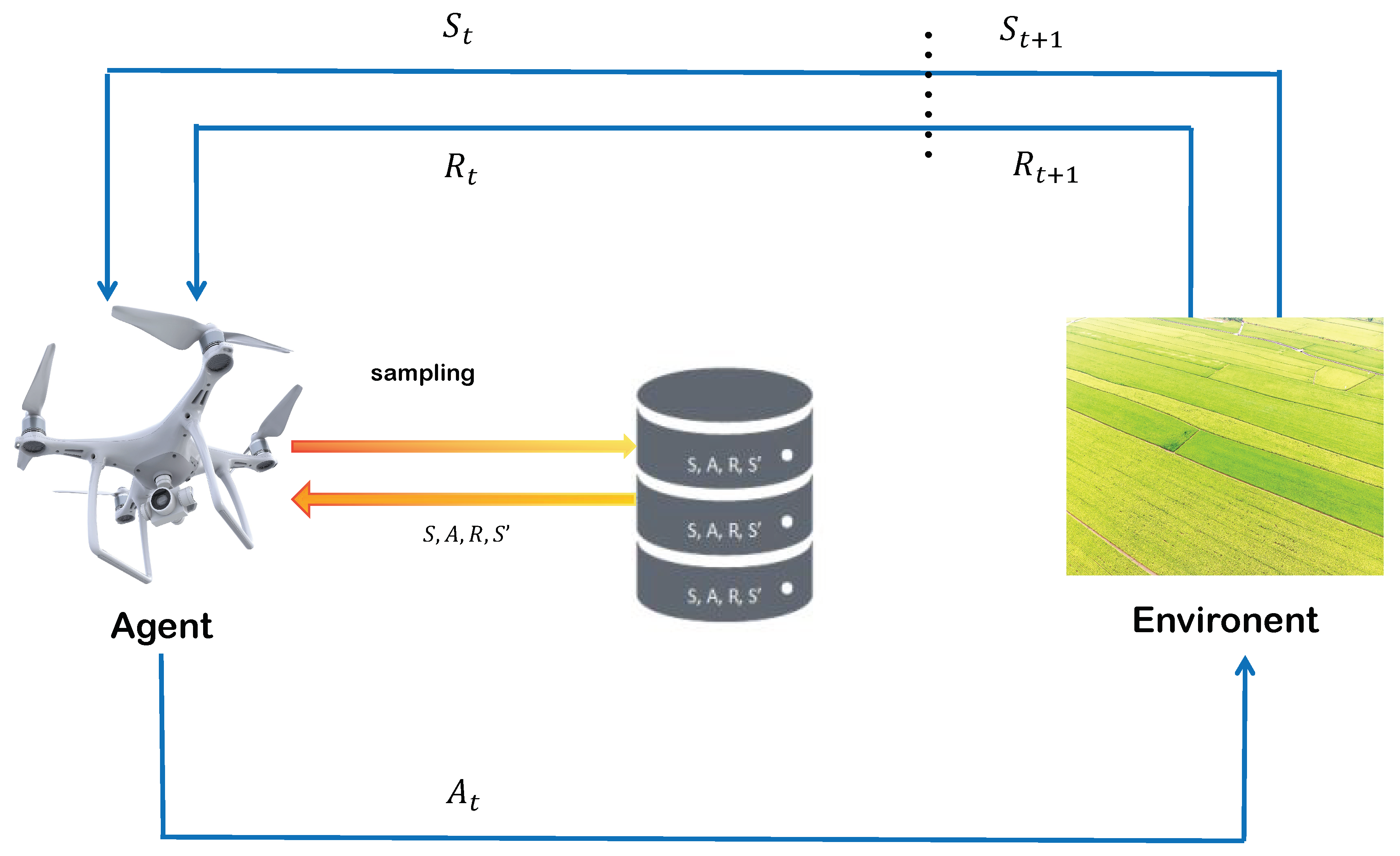
Figure 3.
(a) The overall framework of the algorithm, with red arrows representing data during the training phase and blue arrows representing data during the execution phase; (b) The internal structure of the Actor network; (c) The internal structure of the Critic network.
Figure 3.
(a) The overall framework of the algorithm, with red arrows representing data during the training phase and blue arrows representing data during the execution phase; (b) The internal structure of the Actor network; (c) The internal structure of the Critic network.
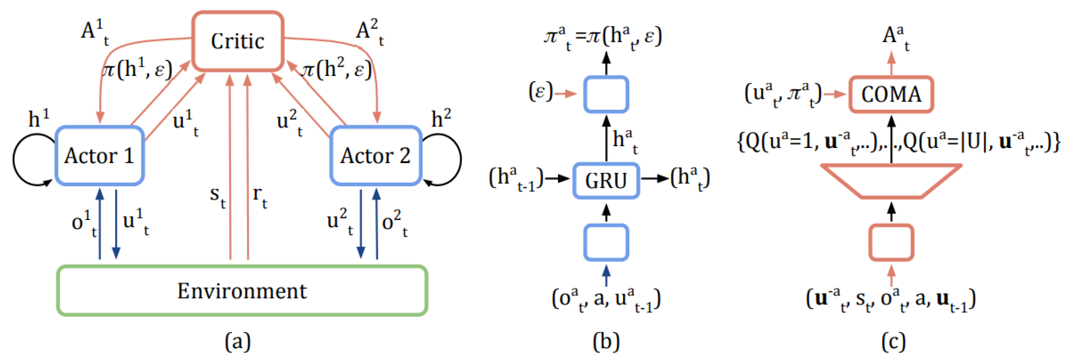
Figure 4.
The figure shows the autoencoder structure, which is divided into the input layer, hidden layer, and output layer.
Figure 4.
The figure shows the autoencoder structure, which is divided into the input layer, hidden layer, and output layer.
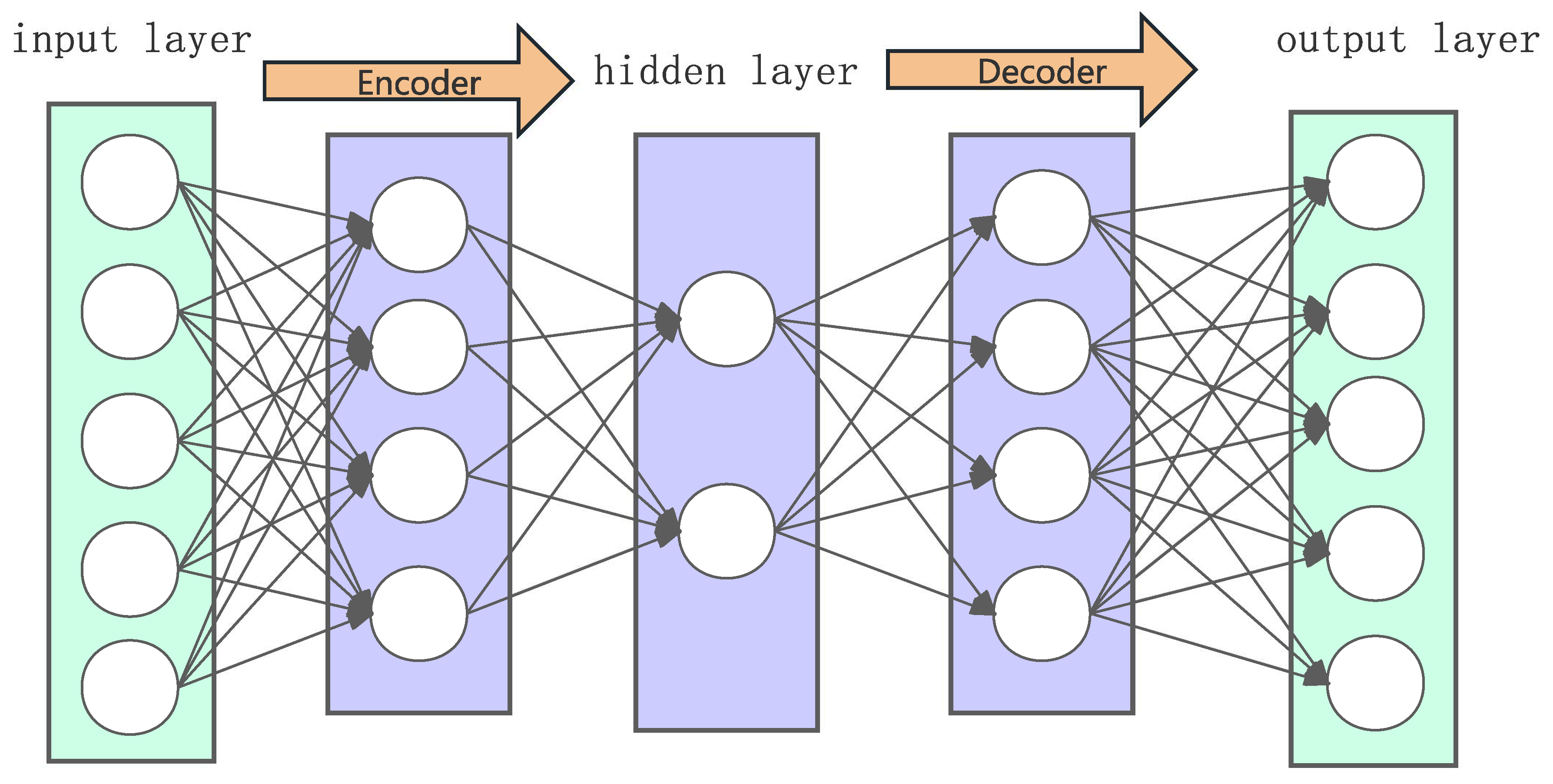
Figure 5.
This diagram depicts the process of deploying and training a multi-UAV system for information gathering. During deployment, UAVs create local maps from their sensor data, which are then processed by an encoder-decoder and an actor network to generate navigation policies. These policies guide the UAVs in collecting data, which is compiled into a global map. During training, the global map is analyzed by a critic network to evaluate the policies’ effectiveness. Feedback from the critic network is used to update the actor network, enhancing future UAV performance.
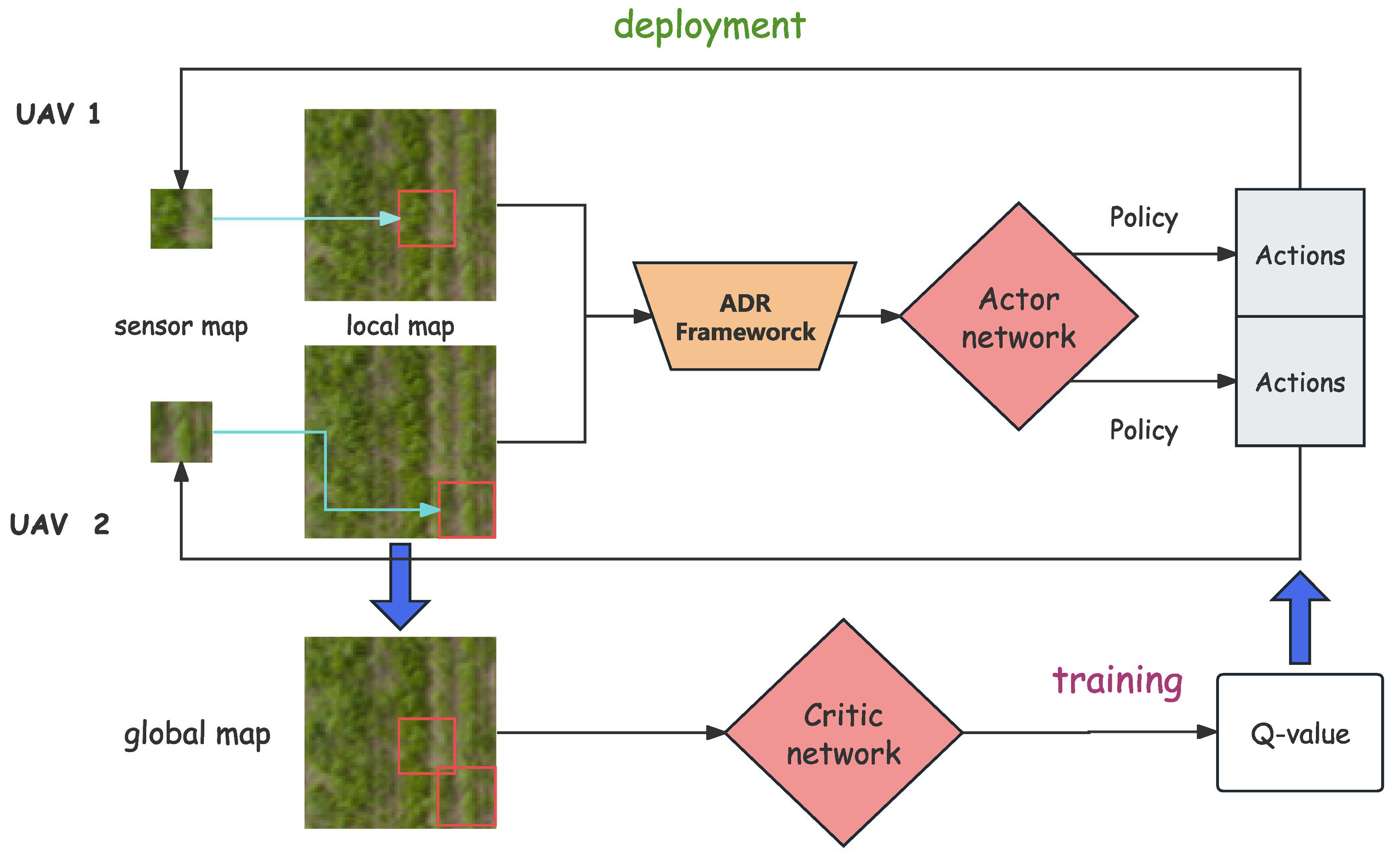
Figure 6.
Illustration of the internal communication of the UAV. The UAVs will interact with each other about their current measurements (shown here as orange, yellow, and purple rectangles). They must be within the communication range to interact, and the range is drawn in white circles in the figure. The green background represents in range, and the red represents out of range.
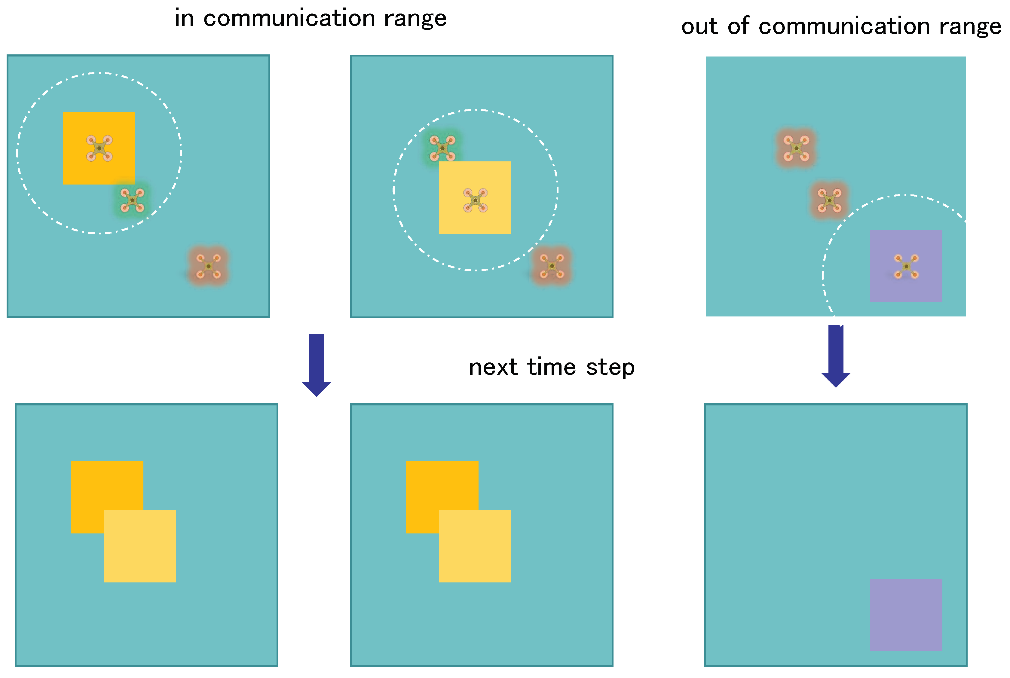
Figure 7.
This is an aerial view of the Chaoyang Campus of Jilin University. The green rectangular building in the centre, called the "Geology Palace," is our area of interest, matching the description of our Scenario 0. Besides the central rectangular building, the two smaller buildings next to it (shown in orange in the image) are also considered secondary areas of interest.
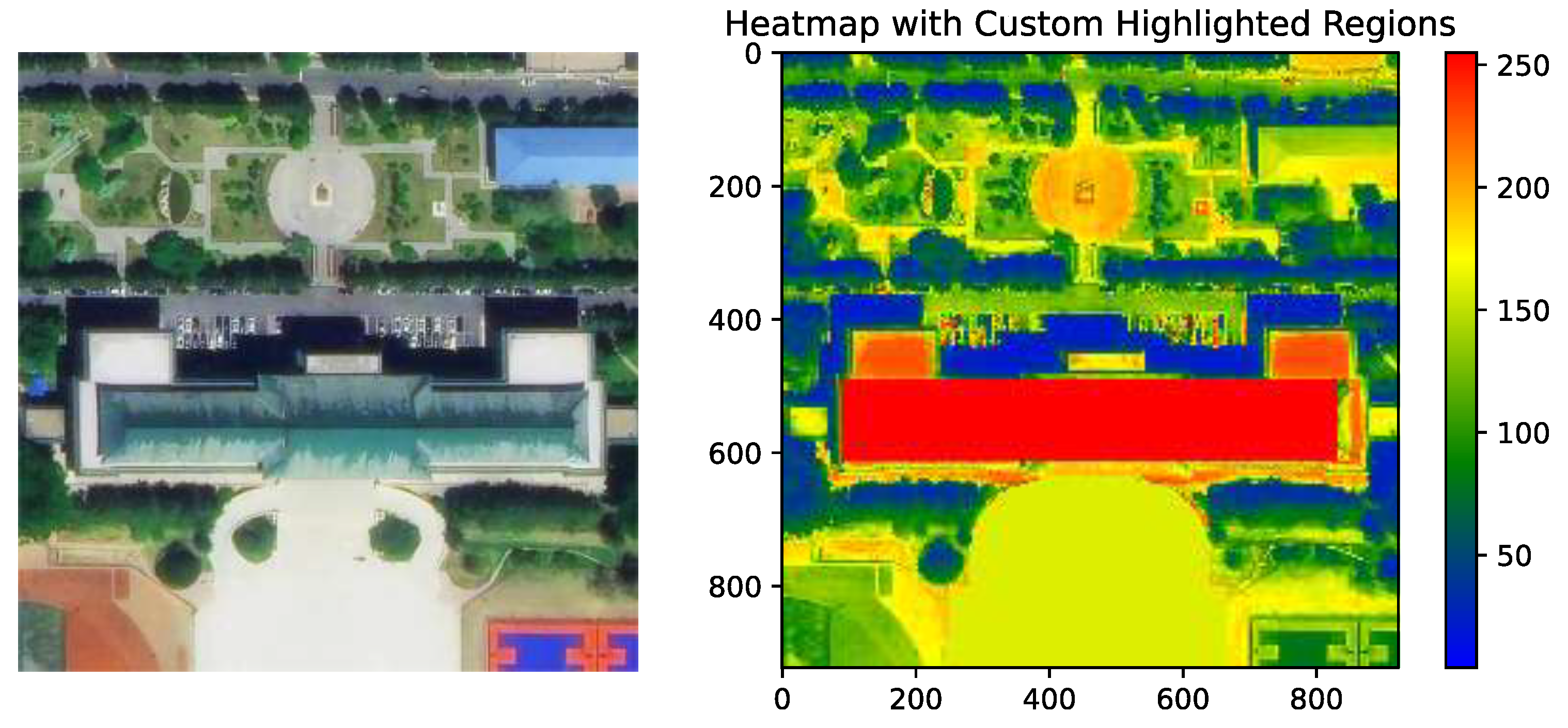
Figure 8.
This is an aerial view of a softball field. The quarter-circle area in the corner is our area of interest, matching the description of our Scenario 1. In this image, we have not designated the highest-interest area (red); only secondary areas of interest are marked. This is because, in real-life scenarios, it is not always possible for every scene to have a highest-interest area.
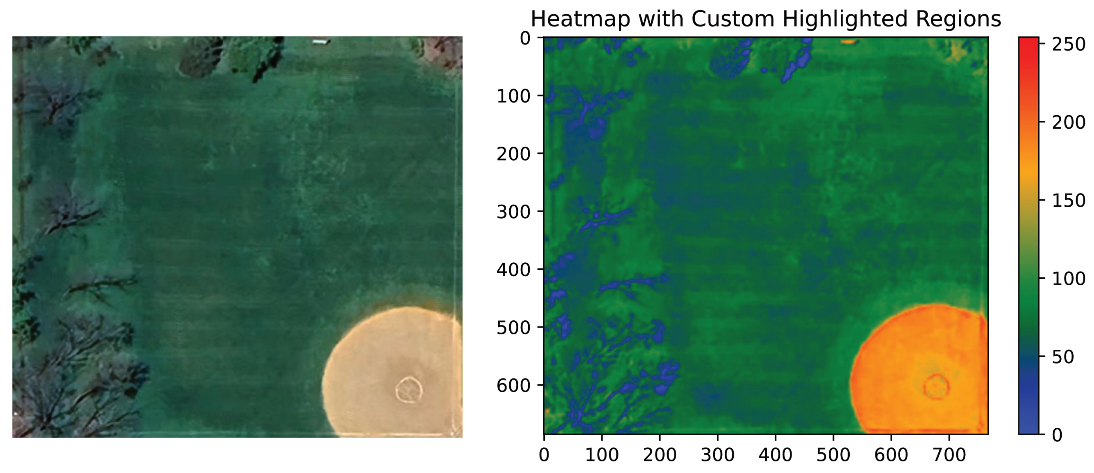
Figure 9.
This is an aerial view of a construction site. The blue rectangular building in the corner is our area of interest, matching the description of Scenario 2. In this image, besides the blue rectangular building being the highest-interest area, we have designated many secondary areas of interest to simulate the real-life scenario where a scene contains numerous areas of interest.
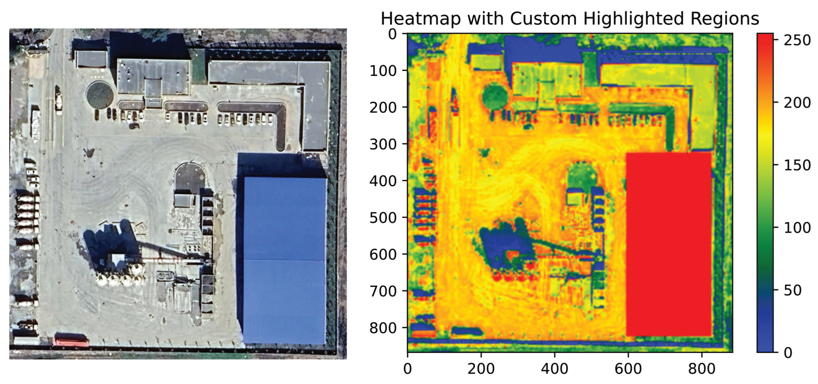
Figure 10.
Reward Trend: Training Performance Across Different Dimensionality Reduction Strategies in Scenario 1.
Figure 10.
Reward Trend: Training Performance Across Different Dimensionality Reduction Strategies in Scenario 1.
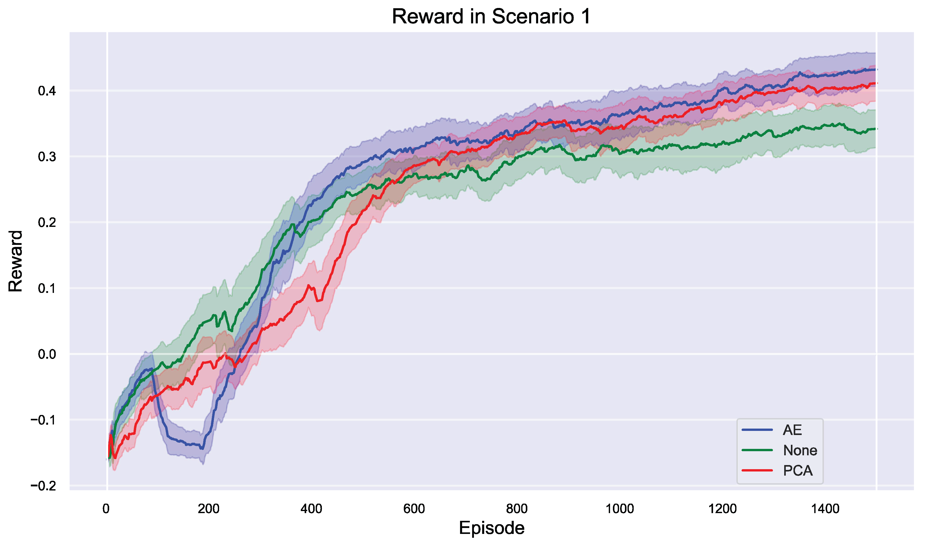
Figure 11.
Q-Value and Entropy Trends: Comparative Analysis of Dimensionality Reduction Strategies in Scenario 1.
Figure 11.
Q-Value and Entropy Trends: Comparative Analysis of Dimensionality Reduction Strategies in Scenario 1.
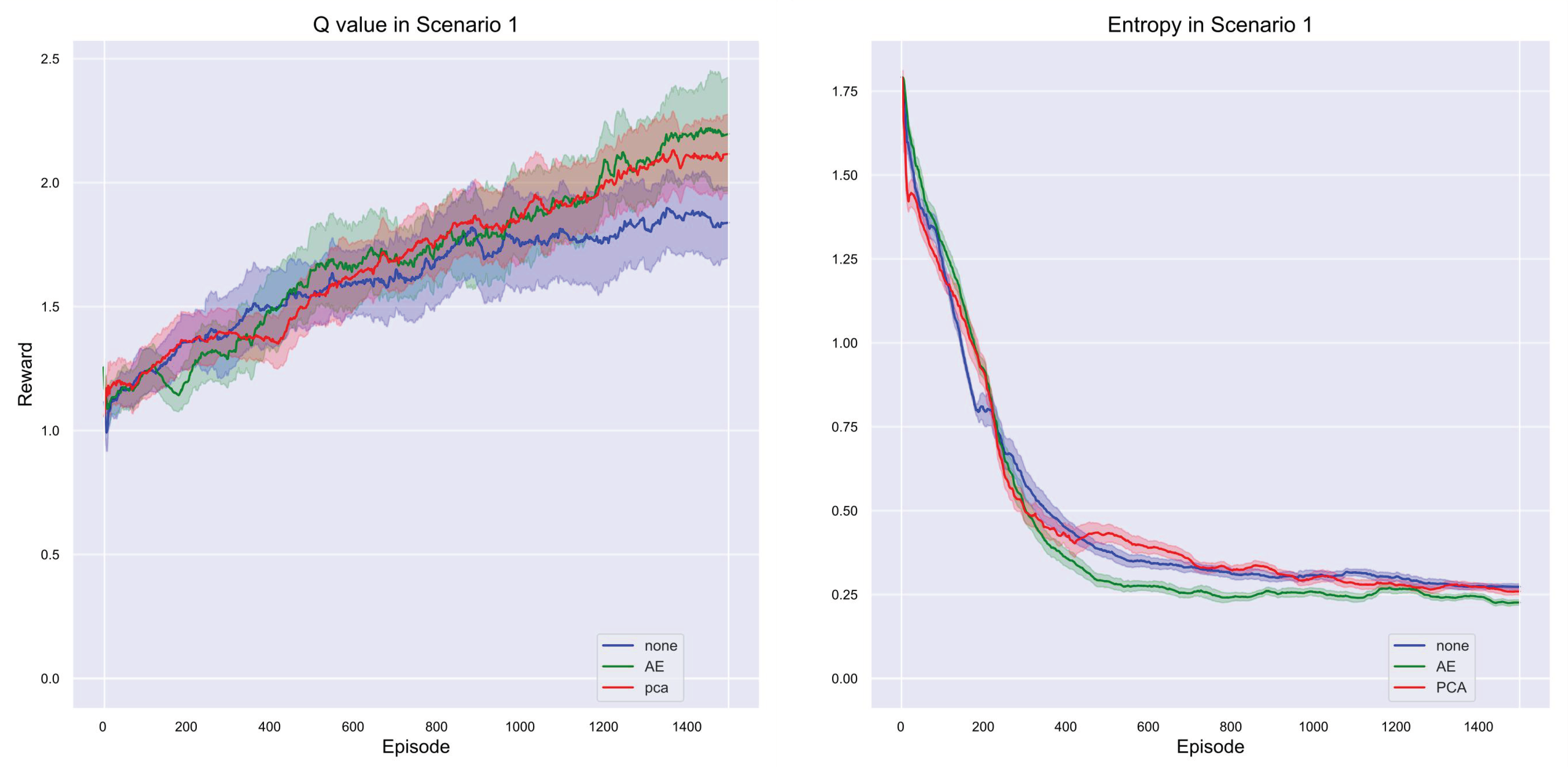
Figure 12.
Reward Trend: Training Performance Across Different Dimensionality Reduction Strategies in Scenario 2.
Figure 12.
Reward Trend: Training Performance Across Different Dimensionality Reduction Strategies in Scenario 2.
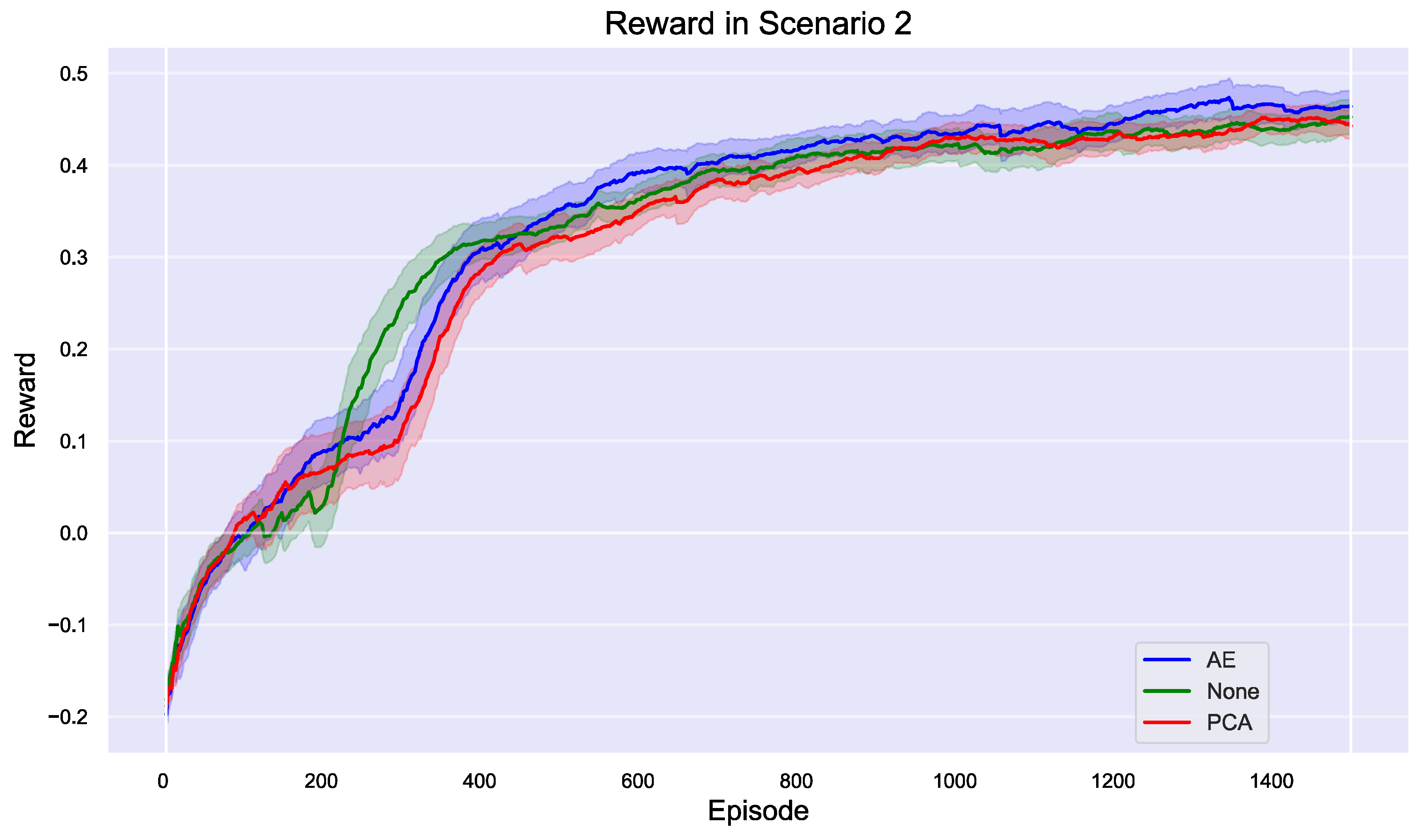
Figure 13.
Q-Value and Entropy Trends: Comparative Analysis of Dimensionality Reduction Strategies in Scenario 2.
Figure 13.
Q-Value and Entropy Trends: Comparative Analysis of Dimensionality Reduction Strategies in Scenario 2.
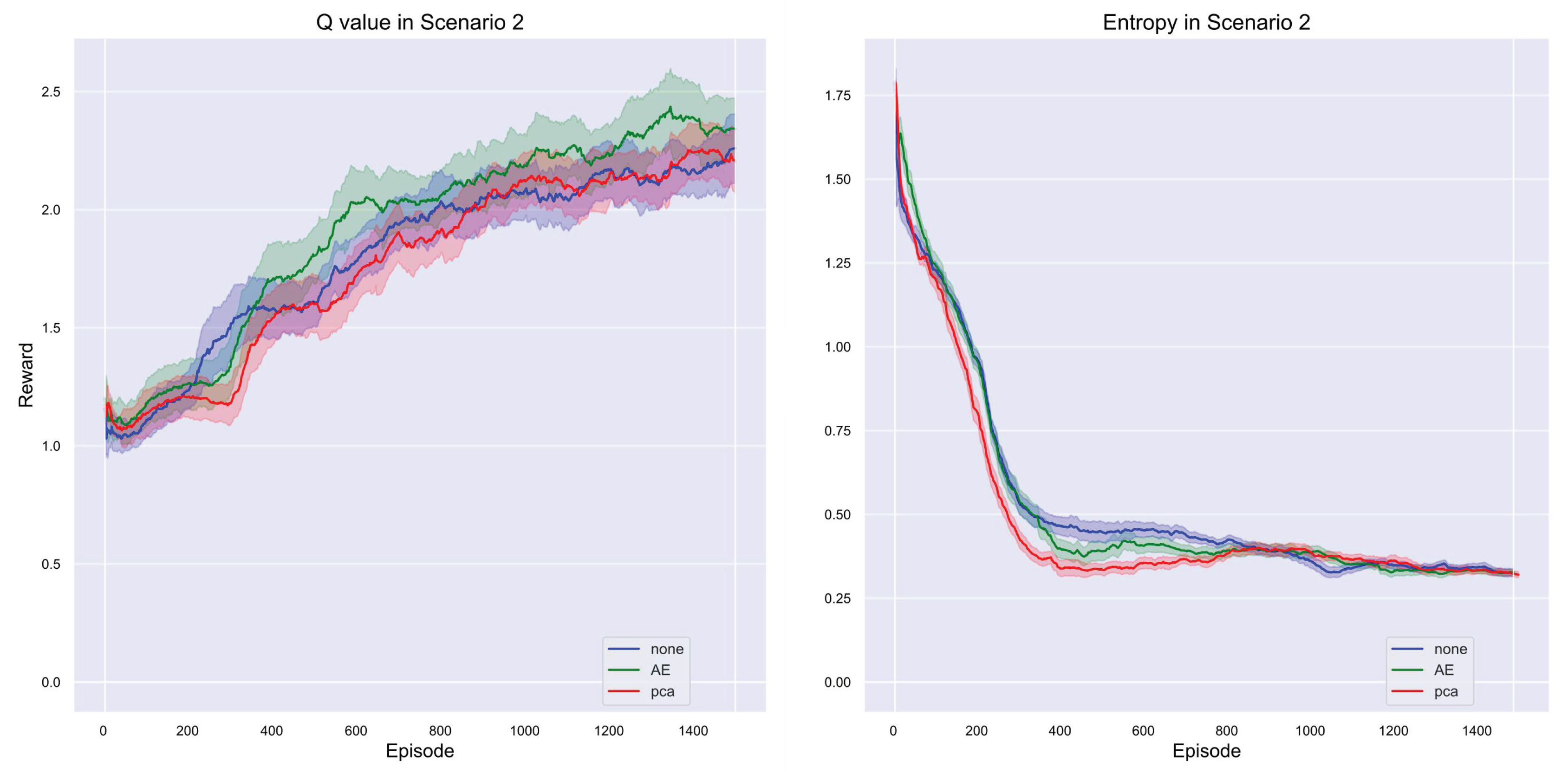
Figure 14.
Reward Trend: Training Performance Across Different Dimensionality Reduction Strategies in Scenario 3.
Figure 14.
Reward Trend: Training Performance Across Different Dimensionality Reduction Strategies in Scenario 3.
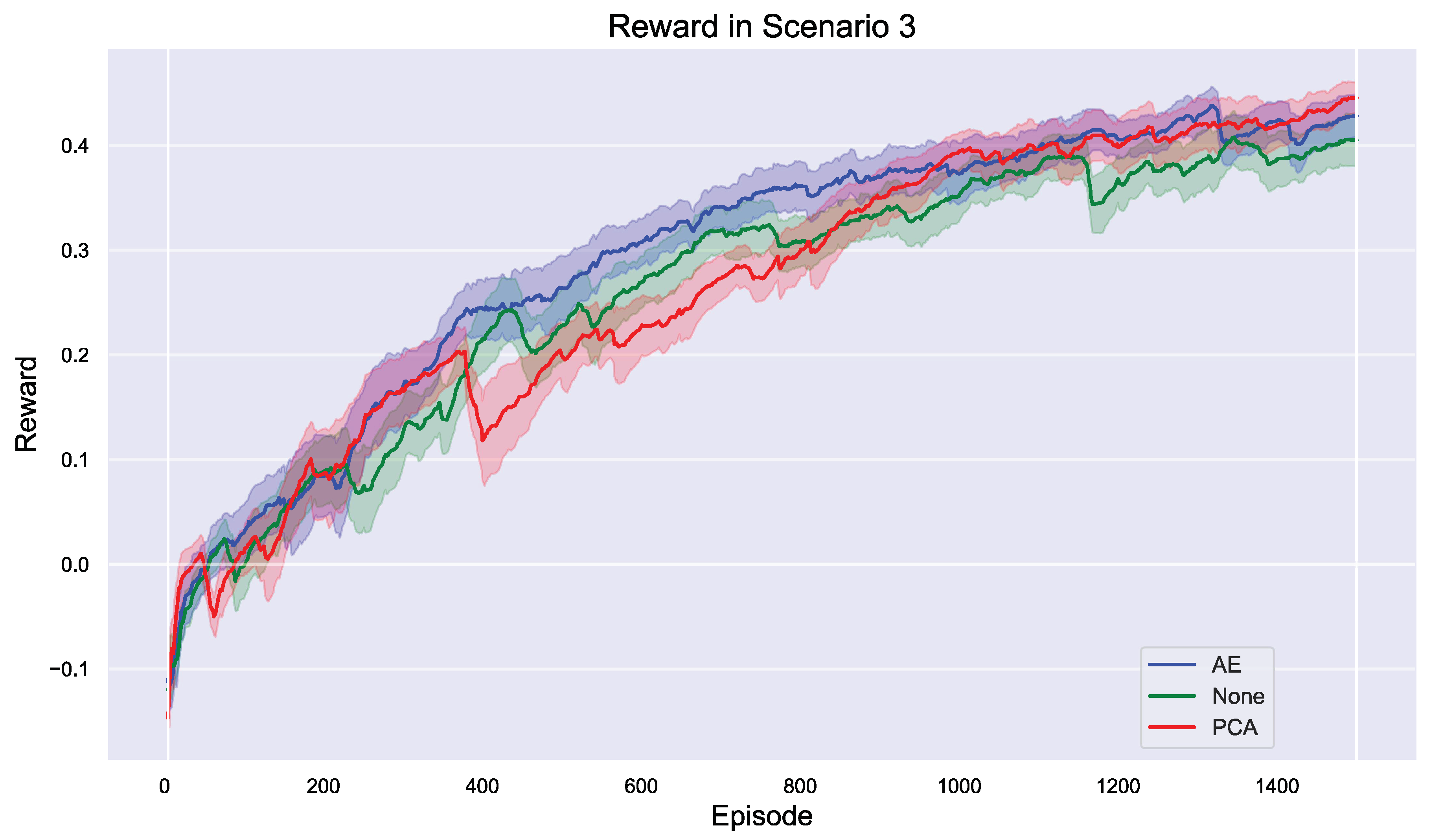
Figure 15.
Q-Value and Entropy Trends: Comparative Analysis of Dimensionality Reduction Strategies in Scenario 3.
Figure 15.
Q-Value and Entropy Trends: Comparative Analysis of Dimensionality Reduction Strategies in Scenario 3.
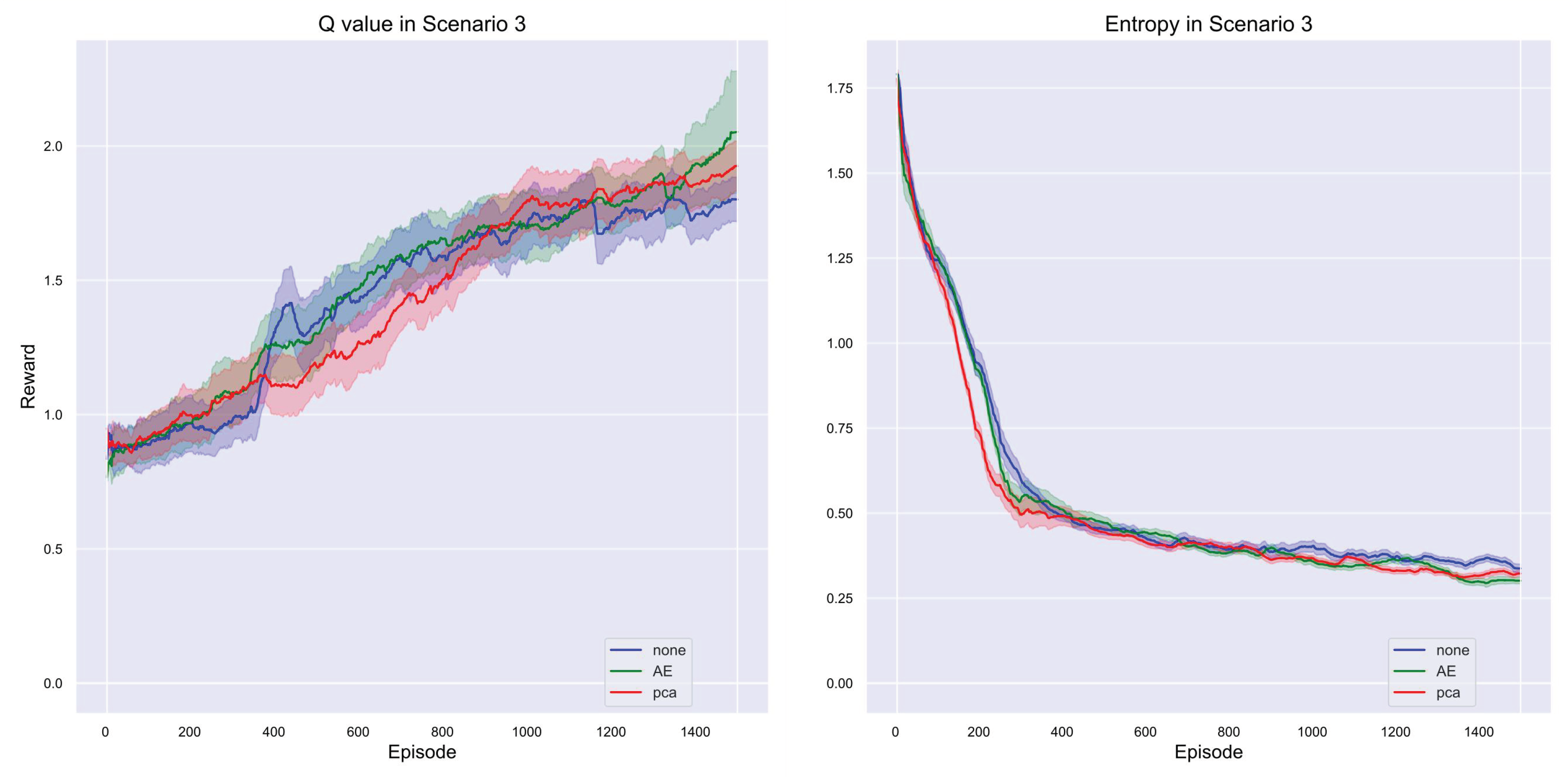

Table 1.
Parameter Configuration Table.
| Parameter Name | Value | Meaning |
|---|---|---|
| 0.99 | Discount factor for future rewards | |
| 0.8 | Weighting factor for future rewards | |
| 0.2 | Parameter in the reward function | |
| 0.5 | Parameter in the reward function | |
| 0.01 | Factor for soft update of target network parameters | |
| learning_rate | 0.00001 | Step size for gradient descent |
| momentum | 0.9 | Factor to accelerate gradient descent in the relevant direction |
| gradient_norm | 10 | Maximum norm for gradients |
| data_passes | 5 | Number of times the dataset is passed through |
| batch_size | 600 | Number of samples processed before the model is updated |
| eps_max | 0.5 | Maximum value for in -greedy strategy, controlling the exploration rate |
| eps_min | 0.02 | Minimum value for in -greedy strategy, controlling the exploration rate |
| sampling_time | 2 | Sampling time in seconds, determines how often the data is collected |
Disclaimer/Publisher’s Note: The statements, opinions and data contained in all publications are solely those of the individual author(s) and contributor(s) and not of MDPI and/or the editor(s). MDPI and/or the editor(s) disclaim responsibility for any injury to people or property resulting from any ideas, methods, instructions or products referred to in the content. |
© 2024 by the authors. Licensee MDPI, Basel, Switzerland. This article is an open access article distributed under the terms and conditions of the Creative Commons Attribution (CC BY) license (http://creativecommons.org/licenses/by/4.0/).
Copyright: This open access article is published under a Creative Commons CC BY 4.0 license, which permit the free download, distribution, and reuse, provided that the author and preprint are cited in any reuse.


