
Submitted:
28 November 2025
Posted:
02 December 2025
You are already at the latest version
Abstract
Among various statistical process control (SPC) methods, control charts are widely employed as essential instruments for monitoring and improving process quality. This study focuses on a new modified exponentially weighted moving average (New Modified EWMA) control chart that enhances detection capability under integrated and fractionally integrated time series processes. Special attention is given to the effect of symmetry on the chart structure and performance. The proposed chart preserves a symmetric monitoring configuration, in which the two-sided design (LCL>0) establishes control limits that are equally spaced around the center line, enabling balanced detection of both upward and downward shifts. Conversely, the one-sided version (LCL=0) introduces a deliberate asymmetry to increase sensitivity to upward mean shifts, which is particularly useful when downward deviations are physically implausible or less critical. The efficacy of the control chart utilizing both models is assessed through Average Run Length (ARL). Herein, the explicit formula of ARL is derived and compared to the ARL obtained from the numerical integral equation (NIE) in terms of both accuracy and computational time. The efficacy of the control chart employing both models is evaluated via Average Run Length (ARL). The explicit formula for ARL is derived and compared to the ARL produced by the numerical integral equation (NIE) regarding accuracy and processing time. The accuracy of the analytical ARL expression is validated by its negligible percentage difference (%diff) in comparison to the results derived using the NIE approach and the display processing time not exceeding 3 seconds. To confirm the highest capability, the suggested method is compared to both the classic EWMA and the modified EWMA charts using evaluation metrics such as ARL and SDRL (standard deviation run length), as well as RMI (relative mean index) and PCI (performance comparison index). Finally, Its examination of US stock prices illustrates performance, employing a symmetrical two-sided control chart for the rapid detection of changes through the new modified EWMA, in contrast to standard EWMA and modified EWMA charts.
Keywords:
average run length
; autoregressive Fractionally Integrated
; control chart
; numerical integral equation
; statistical process control
1. Introduction
Statistical Process Control (SPC) offers a methodical and ongoing strategy for overseeing processes through real-time data to assess whether a system maintains stability or diverges from anticipated performance. Control charts are the fundamental analytical instrument in the SPC framework, allowing practitioners to visualize process variation, swiftly detect anomalous patterns, and execute prompt corrective measures. Their adaptability has facilitated applications in several sectors, including industrial manufacturing [1], financial risk evaluation and economic management [2], environmental monitoring [3], and healthcare systems [4]. Modern data environments often produce intricate time-series signals. Persistence, structural changes, autocorrelation, and long-range dependence distinguish these signals. These characteristics compromise the efficacy of conventional control charts, potentially resulting in asymmetric responses, directional bias, or variable detection capabilities when applied to dynamic, real-world scenarios. These constraints are particularly significant in domains like finance and economics, where the capacity to detect both increasing and decreasing trends with equivalent precision is essential for monitoring volatility, assessing systemic risk, and identifying distinctive economic conditions.
Here, symmetry is essential for design. Symmetrical control limits enable neutrality, stability, and fair detection by responding equally to increase and decrease signals. SPC applications are more reliable in high-volatility, irregularly structured, or changing system contexts due to their symmetric behavior. Consequently, symmetry-preserving control charts provide a solid foundation for monitoring modern real-world systems across disciplines. By applying these ideas to globally influential systems like the U.S. stock market, which is a barometer for macroeconomic circumstances and a major source of financial risk and volatility, control charts become even more important. Market movements affect investor behavior, economic confidence, and indicators of systemic change. Using control charts in this context allows early identification of shifts, monitoring of uncertainty, and an unbiased perspective on price fluctuations. We can now better and faster understand U.S. financial market trends.
Control charts were initially presented by Walter A. Shewhart, [5], who suggested that current sample information may be used to differentiate between common-cause fluctuation and special-cause signals in a process. The simplicity and ease of interpretation of Shewhart charts make them ideal for spotting relatively large changes in the mean process. The cumulative sum (CUSUM) control chart, which counts variances over time, was introduced by Page [6] to make it more sensitive to moderate and minor changes. In a subsequent work, Roberts [7] created the exponentially weighted moving average (EWMA) control chart, which uses a geometrically diminishing weighting structure to enhance sensitivity to subtle or long-lasting shifts in the data. Many extensions of the EWMA framework have been proposed, building on these fundamental advancements. Patel and Divecha [8] introduced the Modified EWMA (Modified EWMA) control chart to enhance sensitivity to subtle process changes. Khan et al. [9] later verified and expanded its performance for a broader range of operating situations. Subsequently, Silpakob et al. [10] enhanced the modified EWMA chart and developed an explicit ARL formula under the AR(p) model. Its efficacy in assessing ARL surpasses that of classic modified EWMA and EWMA charts. Furthermore, recent developments in EWMA-type techniques have brought to light the significance of maintaining chart response symmetry to guarantee balanced detection of upward and downward shifts, thereby lowering directional bias and enhancing accuracy in intricate, correlated, or extremely volatile processes. Symmetric two-sided control charts are essential tools for monitoring process changes because they respond equally to increases and decreases in the signal. The EWMA, modified EWMA, and enhanced new modified EWMA were the main subjects of this investigation. Depending on the monitoring objective, some real-world applications only need one upper or lower limit, even though these charts normally include two. Even while autocorrelation exists in many real systems, conventional charts also imply data independence and uniformity, which can impair detection performance. In some circumstances, specialized or altered control charts are necessary to manage dependency and ensure accurate monitoring.
The ARIMA and ARFIMA models are widely recognized time-series frameworks because they effectively capture key real-world characteristics such as persistence, non-stationarity, and long-memory behavior, which frequently appear in financial and economic data. For the ARIMA model under financial and economic data seen in Sinu et al. [11] as well as ARIMA based on environmental series seen in Hrithik et al. [12]. Pan and Chen [13] and Rabyk and Schmid [14] have further employed these models to examine how dependence structures influence control-chart performance. ARFIMA extends the integer differencing of ARIMA through fractional differencing, allowing a more flexible representation of long-range dependence. With their broad applicability and strong forecasting performance, both models remain essential tools in time-series analysis. In this study, we focus on the ARI and ARFI classes, which are particularly suitable for data exhibiting persistence and long-memory traits features commonly observed in U.S. stock market series characterized by temporal dependence and sustained volatility. Hyung and Franses [15] demonstrated long-memory behavior using daily volatility of the S&P 500, and subsequent ARFI based applications have consistently confirmed this property in U.S. market data.
One important statistic in statistical process control is the average run length (ARL), which is the predicted amount of observations needed before a control chart indicates a state that is out of control. It consists of two parts: , which is best when high since it represents the average run length when the process is under control, and , which is best when low since it reflects the average run length when the process is uncontrolled and needs to be detected quickly when it shifts. In the event that a change or variation takes place in the process, the control chart needs to be able to notice it promptly and indicate whether or not it is necessary to take corrective action or conduct additional investigation. To provide evidence for this assertion, a number of strategies for calculating the ARL have been presented in the scientific literature (see [16,17,18]). These techniques include the Markov chain approach, Monte Carlo simulation, numerical integral equation techniques (NIE), and explicit analytical formulations.
Our primary objective in this research was to assess the efficacy and precision of the explicit formula and the Numerical Integral Equation (NIE) approach in predicting the ARL. It is worth delving further into the relative merits and shortcomings of the two methods, as prior research demonstrated that they can both produce accurate ARL estimations; however, their efficacy differs with respect to model complexity and distributional assumptions. Furthermore, comprehensive study has shown that utilizing the explicit formula can markedly decrease the computation time for determining the ARL.
According to the findings of previous studies, a significant number of scholars have presented the NIE method and established explicit formulas and effectively applied them to any field. For instance, Suriyakat and Petcharat [19] talked about ARL results they got using the NIE method for a CUSUM chart in a seasonal AR model with exogenous variables. Furthermore, Chananet and Phanyaem[20] used the NIE method on an EWMA chart based on an MA model of exogenous variables and showed the ARL performance that went with it. Using real-world economic facts, as a summary, several researchers have also published ARL results obtained using both NIE and explicit formula methods and a range of time-series models. The ARL of the CUSUM control chart was evaluated by Bualuang and Peerajit [21] and Peerajit [22] in 2023. They used the time series model as ARFI and FIMA with external factors. According to the study of Riaz et al. [23], Sunthornwat et al. [24] also came up with an explicit formula for ARL running on the HWMA control chat. These were developed under the MA with exogenous and showed better performance when compared to the CUSUM control chart. Karoon et al. [25] provided explicit ARL formulas for the double EWMA control chart in AR(p). These formulas were then used on a set of economic time series to show how well the process of finding changes works. In their study, Karoon and Areepong [26] demonstrated that the AR(p) model, which includes both trend and quadratic trend components, could derive the Average Run Length (ARL) on the adjusted modified EWMA control chart more effectively than it could on the standard EWMA and modified EWMA control charts. Recently, Karoon and Areepong [27] provided a method that explicitly uses the AR(p) model to derive ARL on the new extended EWMA control chart, which outperforms both standard EWMA and extended EWMA control charts in terms of capability.
Moreover, the literature review indicates that the general AR integrated and fractionally integrated time series models, often referred to as the ARI and ARFI models, have been incorporated into various control charts. For instance, the modified EWMA [28] in 2023 and the double modified EWMA [29] in 2025 are two examples of these control charts. Nevertheless, the new modified EWMA control chart based on ARI and ARFI models has not yet been reported to have any applications. Thus, we showcase the ARL of the new modified EWMA control chart for general ARI and ARFI models, as well as general AR integrated and fractionally integrated time series models. To complete the computation, we used both the precise solution and the NIE approach. The two approaches were compared using the one- and two-sided new modified EWMA control chart for accuracy and calculation speed. Next, the conventional EWMA and modified EWMA control charts were used to compare with the proposed new modified EWMA chart based on both simulated and real-world US stock prices from the S&P 500. Furthermore, this study uses real-life data to demonstrate the change detection capabilities of the new modified EWMA control chart. It was double-checked by displaying a graph to detect changes in control charts.
2. Structures of Control Charts
In the present investigation, the EWMA control charts, the modified EWMA control charts, and the new modified EWMA control charts are all able to detect even minute and modulated alterations in the process. The charts are able to catch deviations that occur in either direction because their upper and lower control limits are positioned in a symmetrical manner around the target value. A signal is created to indicate that the process mean has begun to drift higher or lower when the observed data surpass these restrictions. This signal is generated when the data exceed these limits. This upper–lower symmetrical structure provides a balanced monitoring system that increases the sensitivity of each chart to changes in the mean of the process. In addition, the distinctive upper and lower control limit formula structures of control charts may have an impact on the capacity or sensitivity of these charts to identify changes.
2.1. The EWMA Control Chart
First, the EWMA control chart was initially published in 1959 by Roberts as the first of its kind in research on quality control [7]. Its increased performance compared to previous charts led to its widespread usage in statistical process control (SPC) for tracking and identifying small to moderate process changes. To provide an explan (1) might be used.
where sequence represents observed value at time (t) with exponential white noise. is the exponential smoothing parameter with . And then, represented previously EWMA value, denotes the initial value of the EWMA statistics, and the constant value equal to . It is necessary for the EWMA control chart () to provide evidence of the solution of the mean ( and the variance (, which may be represented as
This system provides the upper control limit (UCL) as indicated in (2) and the lower control limit (LCL) as shown in () to monitor the process, illustrated by the following formulas:
The width of the control limit on the EWMA control chart is denoted by the variable . The EWMA stopping time () is subsequently able to be stated as follows:
The symbols and represent the lower control limit (abbreviated as LCL) and the upper control limit (abbreviated as UCL), respectively.
2.2. The Modified EWMA Control Chart
Second, the modified EWMA chart was initially proposed by Patel and Divecha ([8]). Thereafter, Khan et al. [9] designed it with the purpose of identifying changes in the process that range from minor to moderate magnitude. The following formula can be employed to delineate the statistics of the modified EMWA control chart. It is expressed in (4).
where r is the constant . represented previously modified EWMA value, denotes the initial value of the modified EWMA statistics, and a fixed value: . The solution of the mean () and the variance (), which may be expressed as, must be provided by the modified EWMA control chart (). To explain the modified EMWA chart’s statistics, you can apply this formula.
The following equations demonstrate how this system monitors the process: (5) for the upper control limit (UCL) and () for the lower control limit (LCL).
To represent the stopping time of the modified EWMA control chart, one might likely write it as follows:
Further, if the value of r is equal to 0, the modified EWMA statistic is transformed into the EWMA statistic.
2.3. The New Modified EWMA Control Chart
Third, the new modified EWMA control chart was built as a modification of the modified EWMA chart. This job was accomplished by separating the chart constant r into two distinct values, and . It is possible to characterize the statistic of the new modified EWMA control chart by utilizing the formula that is presented in (7) underneath.
where and are constants . represented previously new modified EWMA value, denotes the initial value of the new modified EWMA statistics, and a fixed value: . It is important to apply the new modified EWMA control chart () in order to offer the information that may be defined as being necessary. The solution of the mean () and the variance () is required. Use this formula to explain the data that are displayed on the new modified EMWA chart.
Equations (8) for the upper control limit (UCL) and () for the lower control limit (LCL) illustrate the manner in which this system carries out the monitoring of the process.
The stopping time of the new modified MEWMA control chart is most likely expressed as follows:
It should be noted that the new modified EWMA statistic is transformed into the modified EWMA statistic when , and back into the EWMA statistic when .
3. Preliminaries of Integrated and Fractionally Integrated Time Series
3.1. The Autoregressive Integrated Model
The autoregressive integrated (ARI) model is a reduced ARIMA framework that retains only the autoregressive and integrated components and omits the moving average term. This standard is suitable for non-stationary time series without significant short-term shock effects that would need a moving average component. In this configuration, the noise term is supposed to be white-noise without autocorrelation. The ARI model’s operator form is shown by Equation (10), which combines the autoregressive polynomial with the differencing operator to describe the process’s dynamic structure.
Expanding the backshift operator, thus
where is constant value, represents autoregressive coefficients, and at . Moreover, the random error is shown to be at period time (t) which is , The degree of differencing to achieve stationarity is denoted by d.
3.2. The Autoregressive Fractionally Integrated Model
By removing the restriction that the differencing order can only accept integer values, the Autoregressive Fractionally Integrated (ARFI) model expands the ARI framework. Due to its adaptability, the model is ideal for depicting long-memory behavior, where the correlation between observations gradually decreases with time. The autoregressive component of the ARFI model explains short-run dynamics, while the fractional differencing operator captures persistent long-term dependency. To illustrate the dynamic structure of the process, Equation (11) combines the autoregressive polynomial with the differencing operator to demonstrate the operator form of the ARFI(p, d) model. The ARFI model generally looks like this:
Therefore, by extending the backshift operator
The parameter d represents the fractional differencing order, which is non-integer and restricted to the interval in this context. As noted by Mcleod and Hipel [30], the fractional differencing parameter typically lies within this range to maintain the stability of the process. Under this condition, the operator can be expressed as an infinite binomial expansion involving successive powers of the backward-shift operator, it can be shown in (11) as follow.
4. Evaluation of Average Run Length for the New Modifed EWMA Control Chart
This section formulates the ARL expressions using two complementary methodologies: the explicit analytical formulation and the Numerical Integral Equation (NIE) technique, both established inside the ARI and ARFI frameworks. Furthermore, it confirms the existence and uniqueness of the ARL derived from the explicit solution.
4.1. Derivation of the ARL Under the ARI() Model
ARI is an autoregressive integrated model of order p, first studied as a particular instance of ARIMA in which the moving-average component is omitted . The current series value is presented as a linear combination of prior observations plus a random error term. Let be observations of the ARI model. An elegant rewriting of the ARI() model is possible with the use of Equations (10) and (12).
where represent the initial values of ARI() model.
First, to obtain the explicit Average Run Length (ARL) for the new modified EWMA control chart under the ARI model.
We can be adjusted by substituting from the ARI in Equation (10) and replacing it in Equation (7). It can result in the following reformulated expression.
where the initial time at , it was set ,and ,
and represents .
So, Equation (7) can be rewritten as
When the process is in control, let us assume that is the symmetrically control limit for . The control limits for are defined by the interval , and this symmetrically controlled limit interval is expressed using the following formulation.
Following is a revised version of the equation that was previously presented, which expresses it in terms of the variable :
Based on the Fredholm integral equation [31], which was employed to create the explicit formula for ARL, let be the explicit ARL formula that is applicable to the new modified EWMA control chart while operating under the ARI model. In the following equation, (13), it is possible to rearrange this item.
Let correspond to , and then and solving for , we obtain . As a result of this, we modified the variable in (13), and the variable is now the solution in (14) in the way that follows:
The mathematical theorem known as the Fixed Point Theorem, discussed in Section 4.3, will verify the solution of the explicit ARL, which has the qualities of existence and uniqueness. It is important to take note of the fact that Equation (14) will accomplish this verification.
After we have demonstrated our existence and uniqueness, Based on the determination of , the solution can be found as follows:
It can be rearranged into the following mathematical equation:
As mentioned earlier, we have defined some variables, which we will discuss further below.
, , and .
In order that we get the equation shown in (15):
Following that, the variable C is considered.
Finally, (16) is replaced in (15), and the solution for the ARL of the new modified EWMA chart under the ARI or called as , that is expressed in (17) as follows:
Consequently, the ARL of the new modified EWMA chart under the ARI can be articulated for the symmetric two-sided control chart utilizing the formulation in (18) as follows:
While, the one-sided new modified EWMA chart under the ARI can be expressed in (19) as follows:
Moreover, for ARLs based on controllable and out-of-control processes, () are set to and . These result in a transformation of the solution to , and in (19), respectively.
Second, the numerical integral equation (NIE) method is used to calculate the Average Run Length (ARL) of the new modified EWMA control chart for the ARI model. When you use the NIE method with quadrature rules, you can evaluate the ARL in a way that is both very accurate and simple to perform on the computer [18].
Let be the ARL of the new modified EWMA chart for the ARI model, computed using the midpoint quadrature rule. Both the two-sided symmetric interval and the one-sided interval with were used to work it out. are the parts that make it up. The quadrature rule is used to set the fixed weights as , and then, represents . Following the steps outlined in equation below, the quadrature rule assesses the approximation of an integral.
We compute using the quadrature rule
The NIE-based ARL can be computed from the matrix equation , which represents the linear system linking the transition probabilities to the expected run length [27],
where and
Changing the order of the previous equation and replacing u with . The NIE approach obtains the numerical approximation of the integral equation for , abbreviated as ARL, as demonstrated in the following.
4.2. Derivation of the ARL Under the ARFI Model
The ARFI model is a fractionally integrated autoregressive process characterized by the differencing parameter. It may assume non-integer values. It is regarded as a specific instance of ARFIMA with signifies that the present value is contingent upon historical observations and a stochastic error component. Fractional differencing engenders long-memory characteristics, rendering ARFI more adaptable than the conventional ARI model. Equations (11) and (12) allow for the concise reformulation of the ARFI process in an autoregressive format for enhanced analysis.
where represent the initial values of ARFI() model, and refer to long-memory process.
First step: To determine the explicit Average Run Length (ARL) for the new modified EWMA control chart under the ARFI model, one must first substitute from the ARFI into Equation (11) and subsequently include it into Equation (7). This action may yield the subsequent reformed phrase.
At the beginning time , was designated as u, as ,
and ℧ is .
Thus, Equation (7) may be reformulated as
Suppose that is the symmetric control limit for when the process is in control state. This symmetric control limit range is expressed using the following formula, and the control limit for is defined as the range .
All steps are expressed as in the ARI process but different parameters.
Here is an updated equation that was previously given, this time using the variable as its expression:
Afterwards, to derive explicit ARL formula, we will use the ARFI model and the new modified EWMA control chart to obtain . This item can be rearranged in the equation given by (22).
Let is , and then and solving for , we obtain . Because of this, the variable is now calculated as the answer in Equation (23) in the following manner:
The explicit ARL’s existence and uniqueness will be verified using the Fixed Point Theorem, explained in Section 4.3. Verification is made easier by solving Equation (23) after solving .
The solution for the ARL of the modified EWMA chart under ARFI, denoted as , is given in (24):
For, the NIE method is used to calculate the ARL of the two-sided new modified EWMA control chart for the ARFI model; It can be called as equation below.
4.3. The Existence and Uniqueness of ARL
Banach’s fixed-point theorem [26] proves the ARL equation’s validity by revealing a unique solution for explicit formulations of the integral equation. Call any continuous function T an operation on the class of all. Example: It showed as:
For a contraction operator T, Banach’s fixed-point theorem states that the fixed-point theorem has a unique solution. The proof of equation for ARI running on the New modified EWMA chart is expressed as:
Proof.
where . □
Therefore, Banach’s fixed point theorem demonstrates the solution exists and is unique.
Moreover, the proof of solution based on ARFI() of the suggested control chart follows proof of the ARI() process mentioned above.
4.4. The Measure Used for Evaluating Capability
Algorithm 1 Computed the explicit ARL and arrived at the control chart coefficients to calculate the ARL on the new modified EWMA chart using the ARI and ARFI models.
| Algorithm 1 The explicit ARL solution for the ARI and ARFI processes running on the new modified EWMA chart |
| Input: |
| - Set the coefficients values of models: and d. |
| - Set the parameters for the new modified EWMA control chart: , and |
| - Set the mean: for the in-control and |
| - Set the mean shifts: , and |
| Output: |
| In-control () |
| - Solve the ARI and ARFI models defined as and with exponential white noise, respectively. |
| - Define the initial parameters and coefficient values. |
| - Set the exponential white noise parameter |
| - Set the lower control limit to for one-sided charts and for symmetrically two-sided charts. |
| - Calculate the upper control limit. 370 is the ARL value for . |
| Out-of-control process () |
| -Determine the mean shift , adjust shifts (). |
| -Compute the ARL values of out-of-control using the explicit formula and the NIE technique. |
After calculating the ARL of two methods, namely the explicit formula and the NIE algorithm:
The next step in evaluating a control chart is to look at its ARL. Here, we begin with the absolute percentage difference (), which contrasts the ARL values ( and ) from the explicit solution with those ( and ) from the NIE method for the ARI and ARFI models, respectively. It can be calculated from the equation in (26) below.
Evaluations of efficiency like SDRL are used with ARL to assess control chart capability in detecting out-of-control circumstances [32]. The SDRL for an in-control and out-of-control processes are calculated as follows:
where, the was set at 370, and the corresponding , evaluated using (27), approximates this value. Control charts with smaller and values can detect shifts in the process mean, leading to better performance.
Moreover, the Performance Comparison Index (PCI).and the Relative Mean Index (RMI) are the main indicators used to evaluate the control charts’ performance in this study. These metrics give a thorough assessment of the charts’ capability to detect process alterations. One important statistic for comparison is the PCI [33], which ranks control charts according to how efficient they are in comparison to the top-performing chart. It is represented in (28) and is defined as the ratio of a particular chart’s AEQL to the lowest AEQL among all charts evaluated.
A PCI number closer to 1 indicates better capability, which allows for quicker detection of out-of-control situations with less loss.
The RMI [29] adds a primary measure of detection improvement across charts, allowing for further technique differentiation. Better process shift sensitivity with lower RMI values (around 0) boosts performance ranking. It can be calculates as in (29) below.
where is the total number of mean shift values used in the evaluation, is the out-of-control ARL when the process mean shift is equal to , and is The lowest ARL value among all charts being compared in .
Here, the Average Extra Quadratic Loss (AEQL) [33] is utilized as a supporting statistic that is employed in the computation of PCI. The AEQL quantifies the average extra loss, which can be calculated using the following formula. As can be seen below.
where, is the total number of shift values from , is the mean shift value, and is the out-of-control ARL at shift . Lower values of the AEQL correspond with lower values of the PCI, which is an indication that the chart is performing more effectively overall.
5. Results and Discussion
5.1. Numerical Findings
Simulation investigations on the new modified EWMA chart compare the efficiency of the NIE technique with that of the explicit formula for the ARI and ARFI models. As mentioned in Algorithm 1, the initial step in comparing the ARL of the two methods was to determine that represents the in-control and represents the out-of-control. The NIE for ARL is created using the division point amount, or 500. The findings are likely shown in Table 1. Please be aware that the findings derived from the two distinct approaches were calculated with the aid of a machine that was operating on Windows 10 (64-bit) and had the following specifications: an Intel Core i5-8250U CPU (1.60 GHz, up to 1.80 GHz) and 4 GB of RAM. The results demonstrate that the ARL values, derived from the ARI model with and , can be expressed for both one-sided and symmetrically two-sided charts, with UCL values of 0, , and . While Table 2 shows the ARL results from running under the ARFI process. It is expressed to set long memory that determined different means at . The accuracy of the results from both tables was measured using the , which indicated excellent accuracy, approaching 0 in all situations. Nevertheless, the explicit formula outperforms NIE in terms of performance since it calculates practically quickly due to its much lower computing time requirements. In contrast, NIE takes more time, always ranging from 2 to 3 seconds. In the future, it makes sense to compare control charts using the explicit ARL formula. The following step involves comparing the efficacy of the new modified EWMA control to the classic EWMA and modified EWMA control charts on the basis of several different situations. This comparison is performed under the ARI and ARFI models, with the explicit formula being used to determine the average run length (ARL). Additionally, the Standard Deviation of Working Length (SDRL) serves as a complementary metric to the ARL, helping to compare the ability to detect performance changes in the process. The results presented by the SDRL can be expressed similarly to the ARL values in all situations.
The results presented in Table 3 and Table 4 illustrate a comparative analysis of the efficiencies of the EWMA, modified EWMA, and new modified EWMA charts across various parameters, with the parameter set for all charts being . The lower control limit is fixed at 0, indicating a one-sided chart, and fixed at 0.5, indicating a two-sided chart; these are expressed in Table 3 and Table 4, respectively. Furthermore, d is fixed at 1 and 2 under the ARI model. The new modified EWMA chart establishes constants , , , and , whereas the EWMA and modified EWMA are defined with and 2, respectively. In every instance across all models, the findings demonstrated that the new modified EWMA chart exhibited reduced and compared to the EEWMA and EWMA control charts when was held constant. Furthermore, the modified EWMA chart with a diminished , specifically in this study, yielded the lowest values for and . This decrease is evidenced by superior capabilities as compared to EWMA and modified EWMA charts.
Table 5 and Table 6 summarize the capability results of the control charts inside the ARFI model, yielding findings congruent with those derived from the ARI model in Table 3 and Table 4. In these assessments, the lower control limit (LCL) is established at 0 for the one-sided chart and at 0.5 for the two-sided chart, as indicated in Table 5 and Table 6, respectively. This study fixed the differencing parameter at and , both of which are within the fractional range . These values signify long-memory behavior, indicating that previous observations have a gradually diminishing impact on the current process, leading to sustained dependency over time. The findings indicate that the new modified EWMA chart with parameters (, ) exhibited the lowest ARL1 and SDRL1 across all scenarios, succeeded by the new modified EWMA chart with (), (), the modified EWMA, and the EWMA charts, respectively. The above results still indicate the new modified EWMA chart’s better performance.
The PCI and RMI, which were calculated using the ARL values, were employed to illustrate that the new modified EWMA control chart performed exceptionally well, which served to corroborate the abilities of the control charts. Moreover, the new modified EWMA control chart, which uses much less than , gives the values less than the new modified EWMA control chart, which uses near . This outcome indicated that the new modified EWMA control chart, which uses much less than , is an alternative chart for evaluating the efficacy of several control charts in this study’s implementation of real-world datasets.
5.2. Empirical Application
The U.S. stock prices hold considerable importance in the global financial arena due to the U.S. stock market being the largest, most liquid, and most important market worldwide. Fluctuations in U.S. stock prices not only signify the performance, stability, and profitability of large firms but also act as a predictive indication of macroeconomic circumstances, investor expectations, and worldwide economic mood. The S&P 500, including 500 prominent U.S. corporations, serves as a well-established benchmark that reflects overall market dynamics and is commonly utilized for investment assessment, portfolio management, and policy analysis. Due to their inherent volatility, long-term dependency, and susceptibility to external shocks in stock prices, they present a realistic and demanding context for assessing statistical monitoring techniques. Thus, employing U.S. stock data enables researchers to assess the efficacy of control charts in identifying structural changes, abrupt shifts, or anomalous patterns in actual time series. This study utilizes three U.S. stock price datasets as representative real-world data sources to validate and assess the efficacy of control charts in monitoring process changes. This research makes use of actual data sets, which include the current U.S. stock prices of Walmart (WMT), Amazon.com (AMZN), and Microsoft (MSFT). All three of these companies are members of the S&P 500 indexes. All of these were fitted using the 82th sample of monthly data from January 2019 to October 2025, searched on the of November, 2025. Three different applications of the U.S. stock price datasets were fitted as ARI and ARFI models using the t-statistics test from the Box-Jenkins technique in the R programming language. The white noise of each model was subsequently checked for its exponential mean using the one-sample Kolmogorov-Smirnov test in SPSS.
Firstly, application 1 was fitted with an ARI() model that shows monthly data of the U.S. stock prices of Walmart (WMT) (Unit:USD). These data were obtained from https://th.investing.com/equities/wal-mart-stores-historical-data. The Box-Ljung test indicated that the model was appropriated (Sig ), and the one-sample Kolmogorov-Smirnov test indicated that the residuals of the ARI() model follow an exponential distribution (Sig ). An acceptable way to write the answer is as follows:
This is the operator form of the ARI() model, with B defined as the backward shift operator.
Second, application 2 was fitted with an ARFI() model that shows monthly data of the U.S. stock prices of Amazon.com (AMZN) (Unit:USD). These data were obtained from https://th.investing.com/equities/amazon-com-inc-historical-data. The Box-Ljung test indicated that the model was appropriated (Sig ), and the one-sample Kolmogorov-Smirnov test indicated that the residuals of the ARFI() model follow an exponential distribution (Sig ). The following is a good way to write it:
Since B is the backward shift operator, this is the operator form of the ARFI() model.
Third, application 3 was fitted with an ARFI() model that shows monthly data of the U.S. stock prices of Microsoft (MSFT) (Unit:USD). These data were obtained from https://th.investing.com/equities/microsoft-corp-historical-data. The Box-Ljung test indicated that the model was appropriated (Sig ), and the one-sample Kolmogorov-Smirnov test indicated that the residuals of the ARFI() model follow an exponential distribution (Sig ). An example of an effective style of writing it is:
In this operator form, B is specified as the backward shift operator, and the ARFI() model is represented.
The results of capability of new modified EWMA, modified EWMA, and EWMA charts under ARI(), ARFI(),and ARFI() that to showed in Table 7, Table 8, and Table 9, respectively. They examined a one-sided control chart with an LCL of 0 and a symmetrically two-sided control chart with an LCL of 0.5, after setting equal to 0.05. Take note that the new modified EWMA chart in this section, which is used with the set , provides a lower ARL and SDRL than the sets and . The findings show that, in every scenario and for every model, the new modified EWMA control chart computed fewer and values compared to the EWMA control chart and the modified EWMA control chart, both a one-sided and a two-sided chart. Based on the PCI and RMI analysis, the New Modified EWMA control chart demonstrates the highest effectiveness in detecting process shifts for both one-sided and two-sided cases. The Modified EWMA chart performs better than the traditional EWMA chart, which shows the lowest effectiveness among the three. The findings were comparable to those from the simulated data in the preceding section, and they validated the capabilities of the new modified EWMA chart. The graphic representation of the PCI and RMI values for all charts under ARI (), ARFI (), and ARFI () clearly demonstrated the capability in Figure 1, Figure 2, and Figure 3.
After that, all control charts were set to in order to identify changes using a two-sided control limit. The EWMA, modified EWMA, and new modified EWMA charts were set to , , and , respectively. In addition, the UCL and LCL controls are symmetrically located around the center line of a symmetric control chart, allowing them to detect process changes equally in both directions. Process monitoring is simplified, and balanced performance is assured, even when detecting little changes, due to this symmetry. In order to identify changes in the process mean, three control charts were utilized to fit three datasets of US stock prices using the 82th sample of monthly data from January 2019 to October 2025. These were achieved by fitting the models followed by the above-mentioned assessment.
As is seen in Figure 4, in the case of the ARI model, the new modified EWMA control chart is able to recognize changes for the first time at the 1st samples, whereas the modified EWMA and EWMA charts are able to identify changes for the first time at 21st and 71st samples, respectively. As shown in Figure 5, the new modified EWMA control chart is able to detect changes for the first time at the 1st samples for the ARFI model, and the modified EWMA is able to detect changes for the first time at the 8th samples, but the EWMA chart is unable to detect changes inside the 82nd samples. Finally, as shown in Figure 6, the ARFI model can be observed with the new modified EWMA control chart at the 1st samples, and with the modified EWMA at the 28th samples as well. However, the EWMA chart fails to detect changes within the 82nd samples of the same ARFI().
6. Conclusions
One way to assess a control chart’s performance using precise formulae and NIE methods is to examine and analyze the ARL computation. This study used both methods to track the ARI and ARFI models with exponential white noise to compute the ARL on the new modified EWMA chart. In contrast to numerical ARL, which requires much longer computation times, analytical ARL performs better and may be computed instantaneously. In the subsequent step, the ARL was used to compare the EWMA and modified EWMA charts instead of the new modified EWMA chart that was created using an explicit formula. Compared to both the conventional EWMA and the modified EWMA charts, it shows greater capability detection in all tests run under the condition’s examination. The findings indicate that the new modified EWMA chart is an effective instrument for detecting minor to moderate shifts utilizing the ARI and ARFI models. Notably, the modified EWMA chart with parameters (, ) demonstrated the lowest ARL1 and SDRL1 across all scenarios, followed by the modified EWMA chart with (), (), the modified EWMA, and the standard EWMA charts, respectively. In addition, the values are lower in the new updated EWMA control chart that utilizes close to , whereas the old control chart uses much more than . Based on these results, the new modified EWMA control chart—which makes far less use of than —is a viable alternative to the control charts used to evaluate the effectiveness of the real-world datasets used in this work. Finally, the new modified EWMA control chart’s capacity was proved to outperform utilizing actual lift data from the US stock prices dataset under the ARFI and ARI models. Further research will employ several models such as ARIMA, SARIMA, ARFIMA, and SARFIMA to determine the ARL of the revised EWMA control chart using an explicit formula. The reason for this is because data from the actual world and data from simulations are different.
Author Contributions
Conceptualization, K.K. and Y.A.; methodology, K.K.; software, K.K.; validation, Y.A.; formal analysis, K.K.; investigation, K.K.; writing—original draft preparation, K.K.; writing—review and editing, K.K. and Y.A.; visualization, K.K.; supervision, Y.A.; funding acquisition, Y.A.; All authors have read and agreed to the published version of the manuscript.
Funding
This research was funded by the National Science, Research, and Innovation Fund (NSRF) and King Mongkut’s University of Technology North Bangkok with Contract no. KMUTNB-FF-69-B-05
Data Availability Statement
This data can be found at https://www.investing.com/equities/united-states.
Acknowledgments
This research was funded by the National Science, Research, and Innovation Fund (NSRF) and King Mongkut’s University of Technology North Bangkok with Contract no. KMUTNB-FF-69-B-05
Conflicts of Interest
The authors declare no conflict of interest.
References
- Malindzakova, M.; Čulková, K.; Trpčevská, J. Shewhart control charts implementation for quality and production management. Processes 2023, 11, 1246. [Google Scholar] [CrossRef]
- Kovarik, M.; Šarga, L.; Klímek, P. Usage of control charts for time series analysis in financial management. J. Bus. Econ. Manag. 2015, 16, 138–158. [Google Scholar] [CrossRef]
- Morrison, L. The use of control charts to interpret environmental monitoring data. Nat. Areas J. 2008, 28, 66–73. [Google Scholar] [CrossRef]
- Suman, G.; Prajapati, D. Control chart applications in healthcare: a literature review. Int. J. Metrol. Qual. Eng. 2018, 9, 5. [Google Scholar] [CrossRef]
- Shewhart, W.A. The application of statistics as an aid in maintaining quality of a manufactured product. J. Am. Stat. Assoc. 1925, 20, 546–548. [Google Scholar] [CrossRef]
- Page, E.S. Continuous inspection schemes. Biometrika 1954, 41, 100–115. [Google Scholar]
- Roberts, S.W. Control chart tests based on qeometric moving averages. Technometrics 1959, 1, 239–250. [Google Scholar]
- Patel, A.K.; Divecha, J. Modified exponentially weighted moving average (EWMA) control chart for an analytical process data. J. Chem. Eng. Mater. Sci. 2011, 2, 12–20. [Google Scholar]
- Khan, N.; Aslam, M.; Jun, C. Design of a control chart using a modified EWMA statistic. Qual. Reliab. Eng. Int. 2016, 33, 1095–1104. [Google Scholar] [CrossRef]
- Silpakob, K.; Areepong, Y.; Sukparungsee, S.; Sunthornwat, R. A new modified EWMA control chart for monitoring processes involving autocorrelated data. Intell. Autom. Soft Comput. 2022, 36, 281–298. [Google Scholar] [CrossRef]
- Sinu, E.; Kleden, M.A.; Atti, A. Application of ARIMA model for forecasting national economic growth: A focus on gross domestic product data. Barekeng J. Ilmu Mat. Terap. 2024, 18, 1261–1272. [Google Scholar] [CrossRef]
- Hrithik, P.M.; Rehman, M.Z.; Dar, A.A.; Wangmo, A.T. Forecasting CO2 emissions in India: A time series analysis using ARIMA. Processes 2024, 12, 2699. [Google Scholar] [CrossRef]
- Pan, J.N.; Chen, S.T. Monitoring long-memory air quality data using ARFIMA model. Environmetrics 2008, 19, 209–219. [Google Scholar] [CrossRef]
- Rabyk, L.; Schmid, W. EWMA control charts for detecting changes in the mean of a long-memory process. Metrika 2016, 79, 267–301. [Google Scholar] [CrossRef]
- Hyung, N.; Franses, P.H. Forecasting time series with long memory and level shifts. J. Forecast. 2005, 24, 1–16. [Google Scholar] [CrossRef]
- Champ, C.W.; Rigdon, S.E. A comparison of the Markov chain and the integral equation approaches for evaluating the run length distribution of quality control charts. Commun. Stat. Simul. Comput. 1991, 20, 191–204. [Google Scholar] [CrossRef]
- Fu, M.C.; Hu, J. Efficient design and sensitivity analysis of control charts using Monte Carlo simulation. Management Science 1999, 45, 395–413. [Google Scholar] [CrossRef]
- Phanyaem, S. Explicit Formulas and Numerical Integral Equation of ARL for SARX(P,r)L Model Based on CUSUM Chart. Mathematics and Statistics 2022, 10, 88–99. [Google Scholar] [CrossRef]
- Suriyakat, W.; Petcharat, K. Exact run length computation on EWMA control chart for stationary moving average process with exogenous variables. Math. Stat. 2022, 10, 624–635. [Google Scholar] [CrossRef]
- Chananet, C.; Phanyaem, S. Improving CUSUM control chart for monitoring a change in processes based on seasonal ARX model. IAENG Int. J. Appl. Math. 2022, 52, IJAM_52_3_08. [Google Scholar]
- Bualuang, D.; Peerajit, W. Performance of the CUSUM control chart using approximation to ARL for long-memory fractionally integrated autoregressive process with exogenous variable. Appl. Sci. Eng. Prog. 2023, 16, 5917. [Google Scholar] [CrossRef]
- Peerajit, W. Developing average run length for monitoring changes in the mean in the presence of long memory under seasonal fractionally integrated MAX model. Math. Stat. 2023, 11, 34–50. [Google Scholar] [CrossRef]
- Riaz, M.; Abbas, Z.; Nazir, H.Z.; Abid, M. On the development of triple homogeneously weighted moving average control chart. CSymmetry 2021, 13, 360. [Google Scholar] [CrossRef]
- Sunthornwat, R.; Sukparungsee, S.; Areepong, Y. Analytical explicit formulas of average run length of homogeneously weighted moving average control chart based on a MAX process. Symmetry 2023, 15, 2112. [Google Scholar] [CrossRef]
- Karoon, K.; Areepong, Y.; Sukparungsee, S. Modification of ARL for detecting changes on the double EWMA chart in time series data with the autoregressive model. Connection Science 2023, 35, 2219040. [Google Scholar] [CrossRef]
- Karoon, K.; Areepong, Y. Enhancing the performance of an adjusted MEWMA control chart running on trend and quadratic trend autoregressive models. Lobachevskii Journal of Mathematics 2024, 45, 1601–1617. [Google Scholar] [CrossRef]
- Karoon, K.; Areepong, Y. The efficiency of the new extended EWMA control chart for detecting changes under an autoregressive model and its application. Symmetry 2025, 17, 104. [Google Scholar] [CrossRef]
- Peerajit, W.; Areepong, Y. Alternative to detecting changes in the mean of an autoregressive fractionally integrated process with exponential white noise running on the modified EWMA control chart. Processes 2023, 11, 503. [Google Scholar] [CrossRef]
- Neammai, J.; Sukparungsee, S.; Areepong, Y. Analytical assessment of the DMEWMA control chart for detecting shifts in ARI and ARFI models with applications. Symmetry 2025, 17, 1889. [Google Scholar] [CrossRef]
- Mcleod, I.; Hipel, K.W. Simulation procedures for Box–Jenkins models. Water Resour. Res. 1978, 14, 969–975. [Google Scholar] [CrossRef]
- Almousa, M. Adomian decomposition method with modified Bernstein polynomials for solving nonlinear Fredholm and Volterra integral equations. Math. Stat. 2020, 8, 278–285. [Google Scholar] [CrossRef]
- Fonseca, A.; Ferreira, P.H.; Nascimento, D.C.; Fiaccone, R.; Correa, C.U.; Piña, A.G.; Louzada, F. Water particles monitoring in the Atacama desert: SPC approach based on proportional data. Axioms 2021, 10, 154. [Google Scholar] [CrossRef]
- Alevizakos, V.; Chatterjee, K.; Koukouvinos, C. The triple exponentially weighted moving average control chart for monitoring Poisson process. Quality and Reliability Engineering International 2023, 38, 532–549. [Google Scholar] [CrossRef]
Figure 1.
PCI and RMI of the EWMA, Modified EWMA, and New Modified EWMA control charts under the ARI(2,2) model, based on monthly Walmart (WMT) stock prices. (a)–(b) show one-sided charts (), while (c)–(d) present two-sided charts ().
Figure 1.
PCI and RMI of the EWMA, Modified EWMA, and New Modified EWMA control charts under the ARI(2,2) model, based on monthly Walmart (WMT) stock prices. (a)–(b) show one-sided charts (), while (c)–(d) present two-sided charts ().
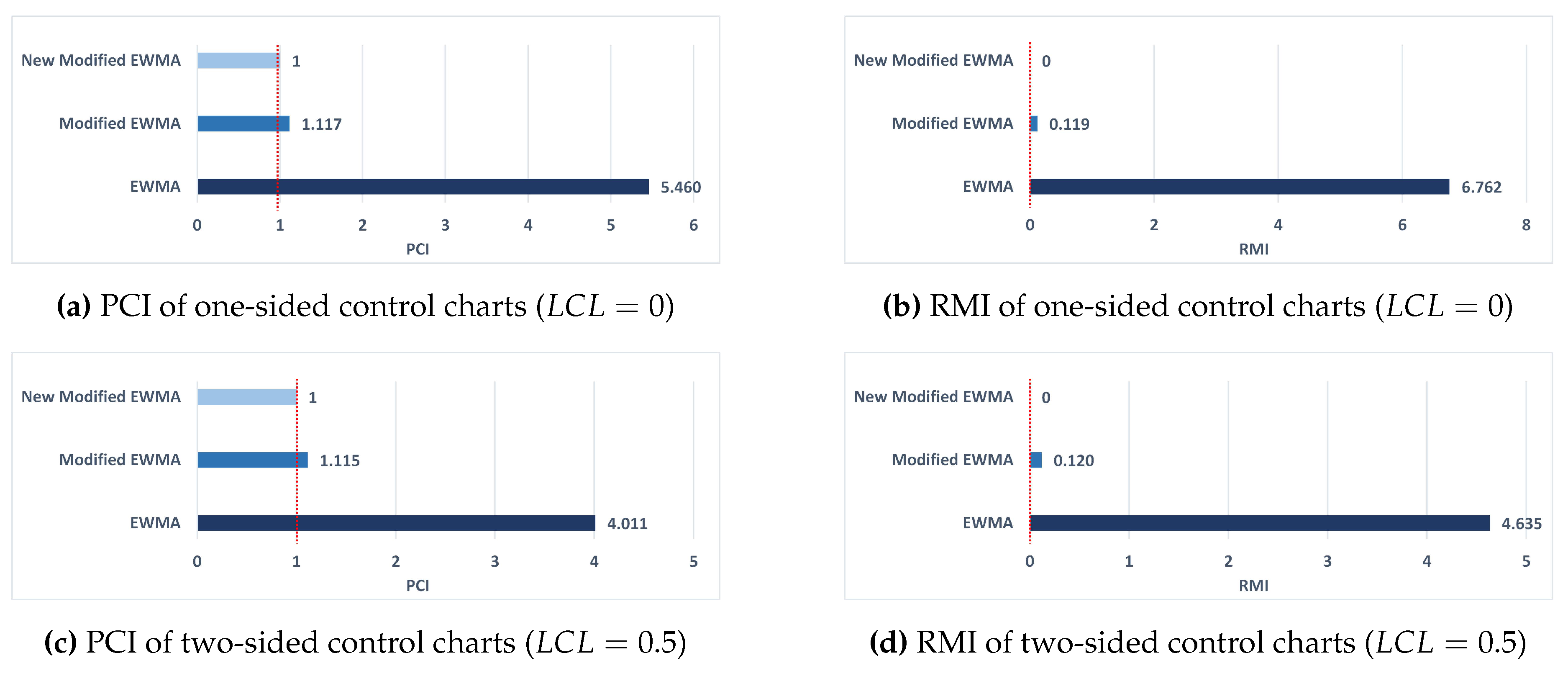
Figure 2.
The PCI and RMI values of the EWMA, Modified EWMA, and New Modified EWMA control charts under the ARFI(1,0.2) model are analytical from monthly Amazon.com (AMZN) stock prices. (a) and (b) illustrate the PCI and RMI for the one-sided control charts (). (c) and (d) display the PCI and RMI for the two-sided control charts ().
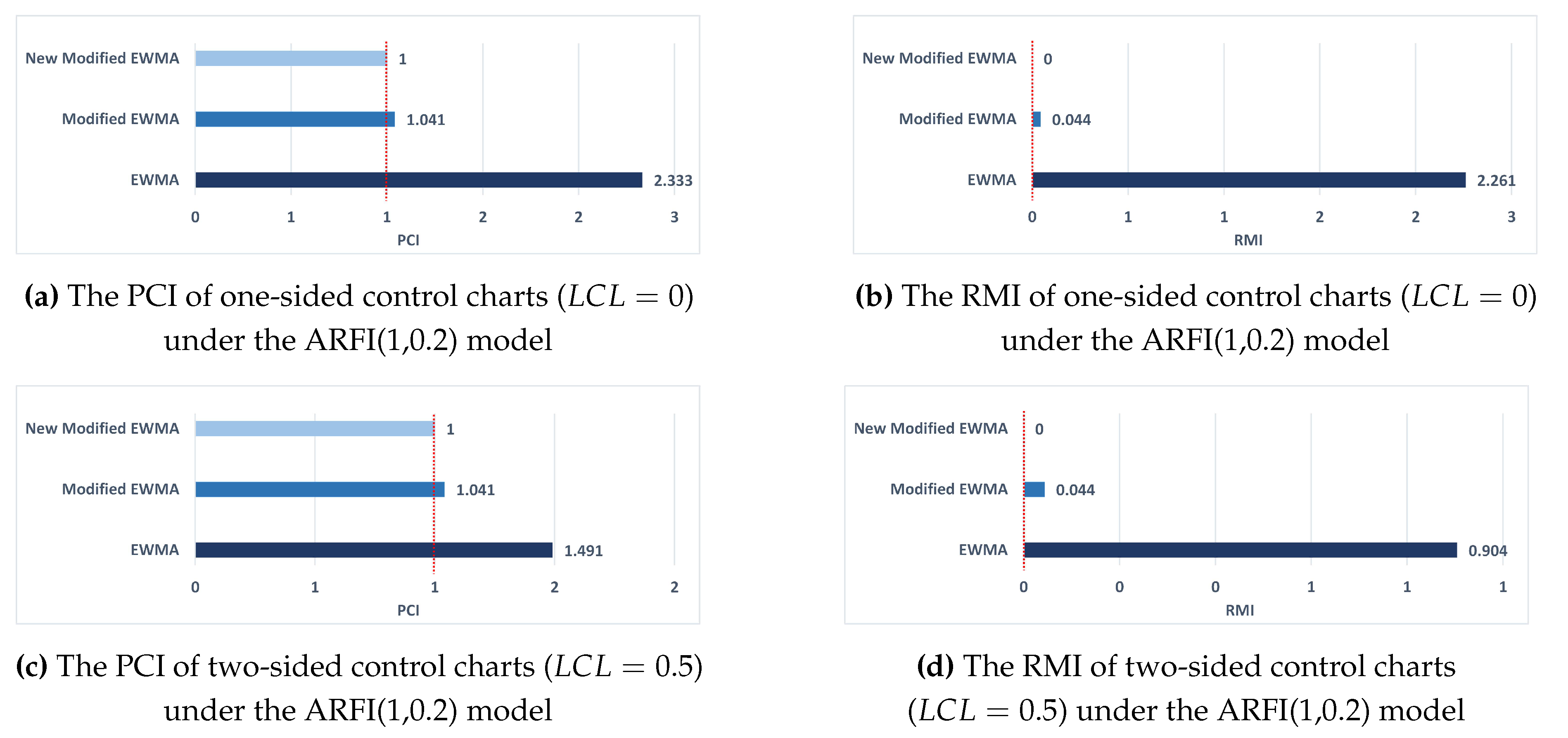
Figure 3.
The PCI and RMI values of the EWMA, Modified EWMA, and New Modified EWMA control charts under the ARFI(2,0.4) model are analytical from monthly Microsoft (MSFT) stock prices. (a) and (b) illustrate the PCI and RMI for the one-sided control charts (). (c) and (d) display the PCI and RMI for the two-sided control charts ().
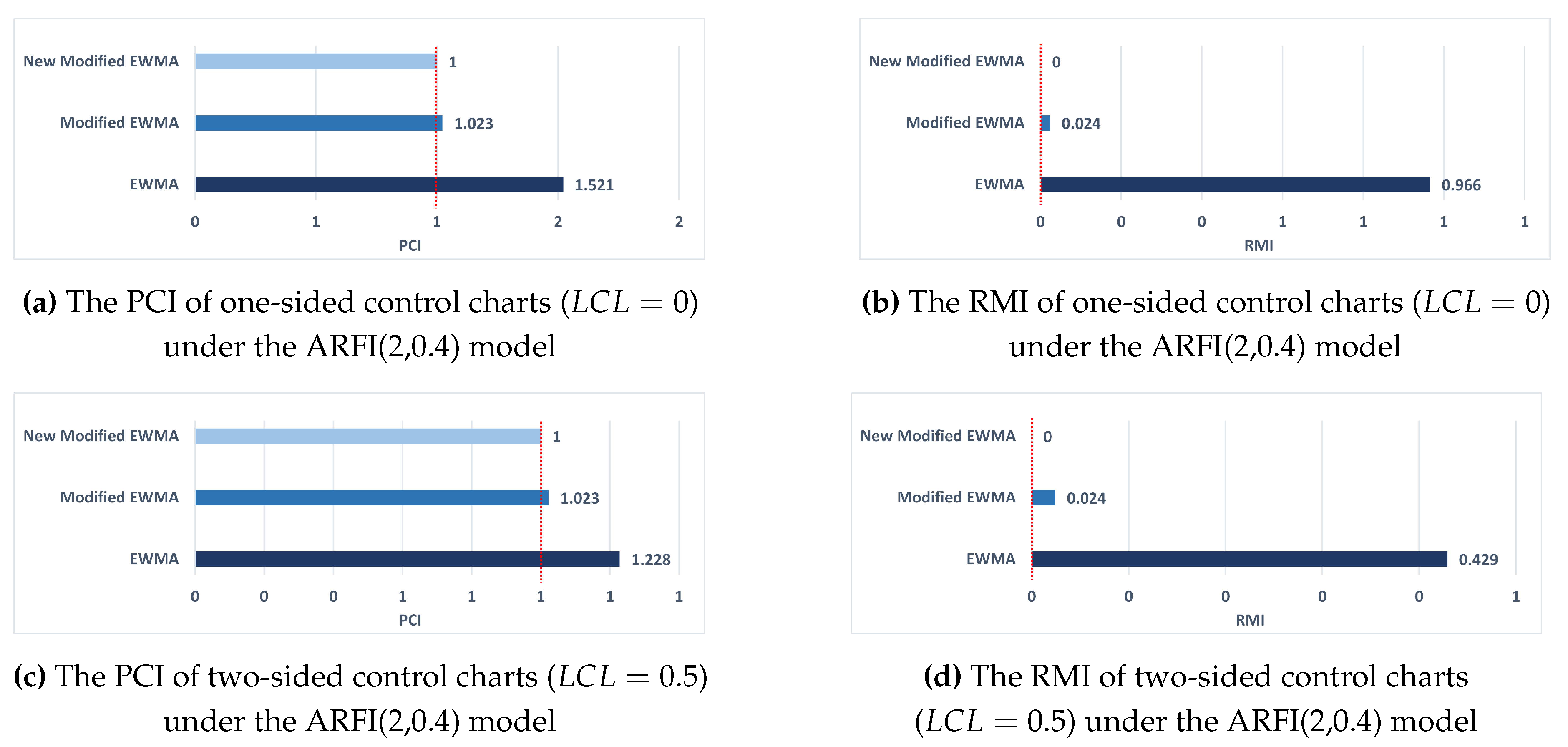
Figure 4.
The capability to detect on symmetric two-sided control charts, namely (a) EWMA, (b) Modified EWMA, and (c) New Modified EWMA under the ARI(2,2) model, is demonstrated using the dataset of monthly Walmart (WMT) stock prices.
Figure 4.
The capability to detect on symmetric two-sided control charts, namely (a) EWMA, (b) Modified EWMA, and (c) New Modified EWMA under the ARI(2,2) model, is demonstrated using the dataset of monthly Walmart (WMT) stock prices.

Figure 5.
The capability to detect on symmetric two-sided control charts, namely (a) EWMA, (b) Modified EWMA, and (c) New Modified EWMA under the ARFI(1,0.2) model, is demonstrated using the dataset of monthly Amazon.com (AMZN) stock prices.
Figure 5.
The capability to detect on symmetric two-sided control charts, namely (a) EWMA, (b) Modified EWMA, and (c) New Modified EWMA under the ARFI(1,0.2) model, is demonstrated using the dataset of monthly Amazon.com (AMZN) stock prices.

Figure 6.
The capability to detect on symmetric two-sided control charts, namely (a) EWMA, (b) Modified EWMA, and (c) New Modified EWMA under the ARFI(2,0.4) model, is demonstrated using the dataset of monthly Microsoft (MSFT) stock prices.
Figure 6.
The capability to detect on symmetric two-sided control charts, namely (a) EWMA, (b) Modified EWMA, and (c) New Modified EWMA under the ARFI(2,0.4) model, is demonstrated using the dataset of monthly Microsoft (MSFT) stock prices.
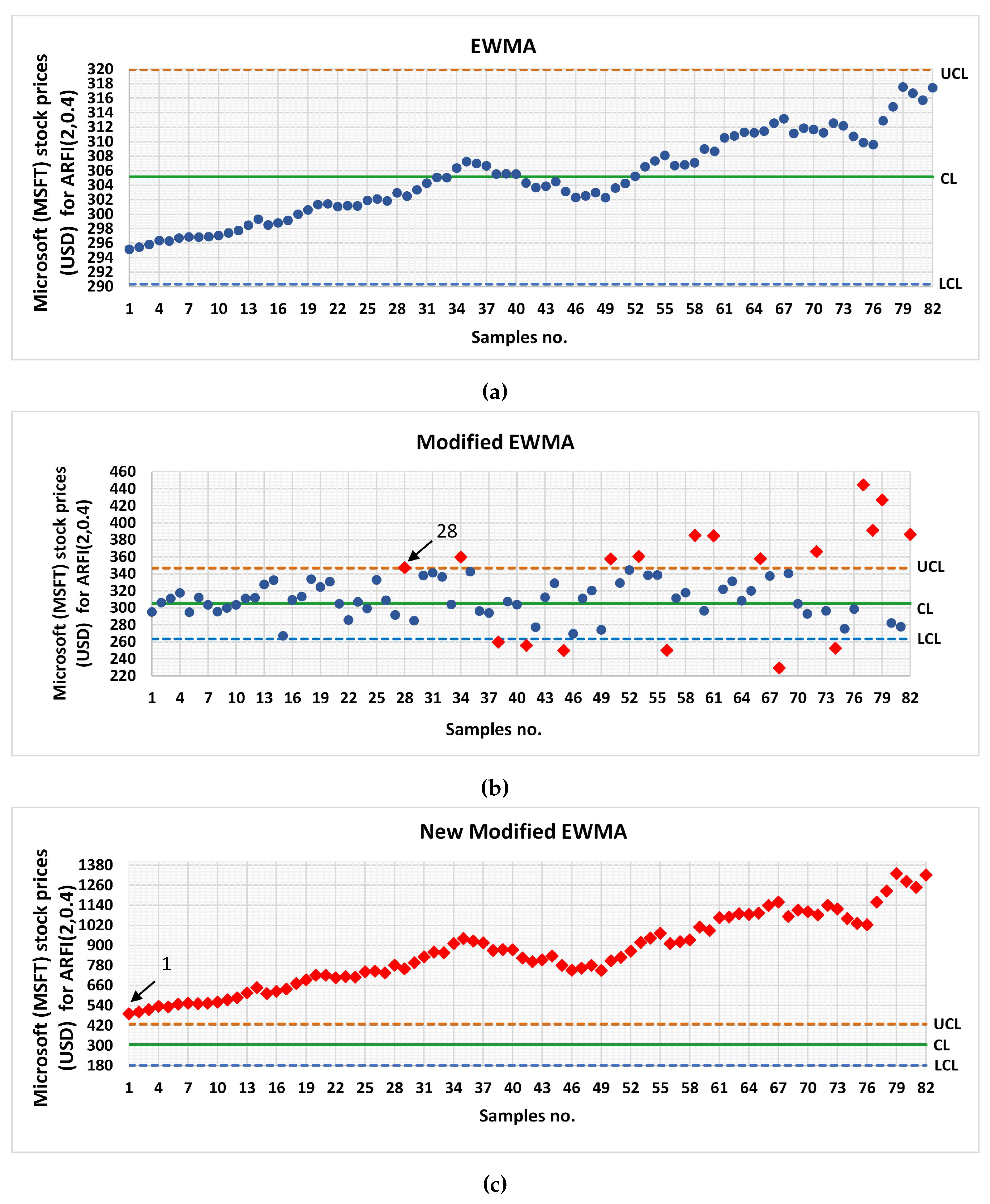

Table 1.
Comparing the accuracy of the ARL on the New Modified EWMA control chart, which are set with lower control limit both one-sided, and two-sided control charts, under the ARI model using the explicit formula against NIE method with determined and .
Table 1.
Comparing the accuracy of the ARL on the New Modified EWMA control chart, which are set with lower control limit both one-sided, and two-sided control charts, under the ARI model using the explicit formula against NIE method with determined and .
| Model | LCL | 0 | 0.1 | 0.5 | ||||||||
| UCL | ||||||||||||
| Methods | ARL | Time | ARL | Time | ARL | Time | ||||||
| ARI(1,1) | 0.05 | 1 | 0.1 | 0 | 370.21370240 | 370.08547158 | 370.17019320 | |||||
| 370.21369836 | 2.375 | 370.08546745 | 2.329 | 370.17018863 | 2.39 | |||||||
| 0.000001090 | 0.000001116 | 0.000001233 | ||||||||||
| 0.0005 | 277.81865343 | 274.57125435 | 261.21200766 | |||||||||
| 277.81865070 | 2.344 | 274.57125160 | 2.421 | 261.21200487 | 2.344 | |||||||
| 0.000000982 | 0.000000999 | 0.000001069 | ||||||||||
| 0.001 | 222.37267580 | 218.29292181 | 201.88494481 | |||||||||
| 222.37267376 | 2.36 | 218.29291978 | 2.359 | 201.88494283 | 2.422 | |||||||
| 0.000000917 | 0.000000929 | 0.000000979 | ||||||||||
| 0.003 | 123.78592235 | 120.09425219 | 105.98808489 | |||||||||
| 123.78592136 | 2.344 | 120.09425122 | 2.359 | 105.98808401 | 2.469 | |||||||
| 0.000000798 | 0.000000804 | 0.000000829 | ||||||||||
| 0.005 | 85.862955829 | 82.942616181 | 72.006860288 | |||||||||
| 85.862955185 | 2.468 | 82.942615555 | 2.406 | 72.006859732 | 2.359 | |||||||
| 0.000000749 | 0.000000754 | 0.000000773 | ||||||||||
| 0.01 | 48.763139703 | 46.924750974 | 40.172384279 | |||||||||
| 48.763139365 | 2.422 | 46.924750647 | 2.39 | 40.172383993 | 2.312 | |||||||
| 0.000000694 | 0.000000698 | 0.000000711 | ||||||||||
| 0.03 | 18.147953507 | 17.442567437 | 14.887866199 | |||||||||
| 18.147953396 | 2.391 | 17.442567330 | 2.343 | 14.887866107 | 2.406 | |||||||
| 0.000000612 | 0.000000614 | 0.000000621 | ||||||||||
| 0.1 | 6.0390546030 | 5.8390012684 | 5.1138777568 | |||||||||
| 6.0390545750 | 2.343 | 5.8390012413 | 2.405 | 5.1138777332 | 2.312 | |||||||
| 0.000000465 | 0.000000464 | 0.000000460 | ||||||||||
| 0.3 | 2.4930107771 | 2.4427301596 | 2.2578068241 | |||||||||
| 2.4930107712 | 2.391 | 2.4427301539 | 2.36 | 2.2578068190 | 2.407 | |||||||
| 0.000000237 | 0.000000235 | 0.000000227 | ||||||||||
| 1 | 1.3456911642 | 1.3383423320 | 1.3104502905 | |||||||||
| 1.3456911636 | 2.359 | 1.3383423314 | 2.39 | 1.3104502900 | 2.343 | |||||||
| 0.000000043 | 0.000000042 | 0.000000041 | ||||||||||
| UCL | ||||||||||||
| Methods | ARL | Time | ARL | Time | ARL | Time | ||||||
| ARI(2,2) | 0.05 | 1.5 | 0.1 | 0.1 | 0 | 370.21370240 | 370.08547158 | 370.17019320 | ||||
| 370.21369836 | 2.375 | 370.08546745 | 2.329 | 370.17018863 | 2.39 | |||||||
| 0.000001090 | 0.000001116 | 0.000001233 | ||||||||||
| 0.0005 | 277.81865343 | 274.57125435 | 261.21200766 | |||||||||
| 277.81865070 | 2.344 | 274.57125160 | 2.421 | 261.21200487 | 2.344 | |||||||
| 0.000000982 | 0.000000999 | 0.000001069 | ||||||||||
| 0.001 | 222.37267580 | 218.29292181 | 201.88494481 | |||||||||
| 222.37267376 | 2.36 | 218.29291978 | 2.359 | 201.88494283 | 2.422 | |||||||
| 0.000000917 | 0.000000929 | 0.000000979 | ||||||||||
| 0.003 | 123.78592235 | 120.09425219 | 105.98808489 | |||||||||
| 123.78592136 | 2.344 | 120.09425122 | 2.359 | 105.98808401 | 2.469 | |||||||
| 0.000000798 | 0.000000804 | 0.000000829 | ||||||||||
| 0.005 | 85.862955829 | 82.942616181 | 72.006860288 | |||||||||
| 85.862955185 | 2.468 | 82.942615555 | 2.406 | 72.006859732 | 2.359 | |||||||
| 0.000000749 | 0.000000754 | 0.000000773 | ||||||||||
| 0.01 | 48.763139703 | 46.924750974 | 40.172384279 | |||||||||
| 48.763139365 | 2.422 | 46.924750647 | 2.39 | 40.172383993 | 2.312 | |||||||
| 0.000000694 | 0.000000698 | 0.000000711 | ||||||||||
| 0.03 | 18.147953507 | 17.442567437 | 14.887866199 | |||||||||
| 18.147953396 | 2.391 | 17.442567330 | 2.343 | 14.887866107 | 2.406 | |||||||
| 0.000000612 | 0.000000614 | 0.000000621 | ||||||||||
| 0.1 | 6.0390546030 | 5.8390012684 | 5.1138777568 | |||||||||
| 6.0390545750 | 2.343 | 5.8390012413 | 2.405 | 5.1138777332 | 2.312 | |||||||
| 0.000000465 | 0.000000464 | 0.000000460 | ||||||||||
| 0.3 | 2.4930107771 | 2.4427301596 | 2.2578068241 | |||||||||
| 2.4930107712 | 2.391 | 2.4427301539 | 2.36 | 2.2578068190 | 2.407 | |||||||
| 0.000000237 | 0.000000235 | 0.000000227 | ||||||||||
| 1 | 1.3456911642 | 1.3383423320 | 1.3104502905 | |||||||||
| 1.3456911636 | 2.359 | 1.3383423314 | 2.39 | 1.3104502900 | 2.343 | |||||||
| 0.000000043 | 0.000000042 | 0.000000041 | ||||||||||
Table 2.
Comparing the accuracy of the ARL on the New Modified EWMA control chart, which are set with a lower control limit at LCL for one-sided and LCL for two-side control charts, under the ARFI model using the explicit formula against NIE method with determined , and .
Table 2.
Comparing the accuracy of the ARL on the New Modified EWMA control chart, which are set with a lower control limit at LCL for one-sided and LCL for two-side control charts, under the ARFI model using the explicit formula against NIE method with determined , and .
| Model | ARFI | ||||||||||
| d | |||||||||||
| (LCL,UCL) | |||||||||||
| Methods | ARL | Time | ARL | Time | ARL | Time | ARL | Time | |||
| 0.15 | 1 | 0 | 370.05357527 | 370.11033031 | 370.14146867 | 370.07644250 | |||||
| 370.05352820 | 2.625 | 370.11025127 | 2.594 | 370.14143910 | 2.484 | 370.07640357 | 2.594 | ||||
| 0.000012722 | 0.000021354 | 0.000007989 | 0.000010519 | ||||||||
| 0.0005 | 284.12295732 | 289.72760017 | 279.24019232 | 282.11358439 | |||||||
| 284.12292850 | 2.501 | 289.72755009 | 2.577 | 279.24017477 | 2.547 | 282.11356086 | 2.608 | ||||
| 0.000010143 | 0.000017286 | 0.000006283 | 0.000008340 | ||||||||
| 0.001 | 230.62640419 | 238.07579658 | 224.23193953 | 227.98309858 | |||||||
| 230.62638450 | 2.485 | 238.07576165 | 2.578 | 224.23192776 | 2.438 | 227.98308263 | 2.438 | ||||
| 0.000008537 | 0.000014670 | 0.000005250 | 0.000006999 | ||||||||
| 0.003 | 131.70181522 | 139.12657992 | 125.56166925 | 129.13741609 | |||||||
| 131.70180790 | 2.469 | 139.12656649 | 2.501 | 125.56166499 | 2.532 | 129.13741022 | 2.5 | ||||
| 0.000005560 | 0.000009649 | 0.000003392 | 0.000004543 | ||||||||
| 0.005 | 92.286586707 | 98.402160317 | 87.309408650 | 90.199015169 | |||||||
| 92.286582677 | 2.5 | 98.402152866 | 2.546 | 87.309406322 | 2.562 | 90.199011949 | 2.563 | ||||
| 0.000004367 | 0.000007572 | 0.000002667 | 0.000003569 | ||||||||
| 0.01 | 52.960178234 | 56.999825876 | 49.725705650 | 51.597718573 | |||||||
| 52.960176561 | 2.484 | 56.999822779 | 2.547 | 49.725704684 | 2.516 | 51.597717236 | 2.5 | ||||
| 0.000003159 | 0.000005432 | 0.000001943 | 0.000002589 | ||||||||
| 0.03 | 19.917023026 | 21.600627002 | 18.587945087 | 19.355089975 | |||||||
| 19.917022617 | 2.452 | 21.600626253 | 2.562 | 18.587944848 | 2.562 | 19.355089646 | 2.532 | ||||
| 0.000002056 | 0.000003468 | 0.000001285 | 0.000001697 | ||||||||
| 0.1 | 6.6844575161 | 7.2595651570 | 6.2336730700 | 6.4934834643 | |||||||
| 6.6844574268 | 2.501 | 7.2595649948 | 2.515 | 6.2336730177 | 2.499 | 6.4934833925 | 2.515 | ||||
| 0.000001336 | 0.000002234 | 0.000000839 | 0.000001105 | ||||||||
| 0.3 | 2.7642652085 | 2.9814943402 | 2.5952426678 | 2.6924955062 | |||||||
| 2.7642651899 | 2.703 | 2.9814943060 | 2.485 | 2.5952426570 | 2.531 | 2.6924954914 | 2.563 | ||||
| 0.000000673 | 0.000001147 | 0.000000415 | 0.000000553 | ||||||||
| 1 | 1.4500558766 | 1.5261690885 | 1.3919495203 | 1.4252423551 | |||||||
| 1.4500558747 | 2.516 | 1.5261690847 | 2.562 | 1.3919495192 | 2.578 | 1.4252423536 | 2.499 | ||||
| 0.000000135 | 0.000000245 | 0.000000079 | 0.000000108 | ||||||||
| d | |||||||||||
| (LCL,UCL) | |||||||||||
| Methods | ARL | Time | ARL | Time | ARL | Time | ARL | Time | |||
| 0.15 | 3.5 | 0 | 370.04780163 | 370.09273890 | 370.18132219 | 370.02034117 | |||||
| 370.04780141 | 2.578 | 370.09273834 | 2.594 | 370.18132201 | 2.578 | 370.02034087 | 2.688 | ||||
| 0.0000000587 | 0.0000001520 | 0.0000000479 | 0.0000000786 | ||||||||
| 0.0005 | 212.50418511 | 221.26755323 | 210.62842029 | 215.17853412 | |||||||
| 212.50418504 | 2.531 | 221.26755301 | 2.594 | 210.62842023 | 2.625 | 215.17853401 | 2.532 | ||||
| 0.0000000371 | 0.0000000980 | 0.0000000292 | 0.0000000499 | ||||||||
| 0.001 | 149.15102108 | 157.90603732 | 147.29195064 | 151.79886834 | |||||||
| 149.15102104 | 2.5 | 157.90603720 | 2.563 | 147.29195061 | 2.547 | 151.79886828 | 2.594 | ||||
| 0.0000000279 | 0.0000000753 | 0.0000000223 | 0.0000000379 | ||||||||
| 0.003 | 68.240909481 | 73.813635601 | 67.079011538 | 69.903749927 | |||||||
| 68.240909469 | 2.469 | 73.813635568 | 2.531 | 67.079011529 | 2.516 | 69.903749911 | 2.625 | ||||
| 0.0000000164 | 0.0000000446 | 0.0000000131 | 0.0000000224 | ||||||||
| 0.005 | 44.384810240 | 48.308784667 | 43.571806944 | 45.550726555 | |||||||
| 44.384810234 | 2.593 | 48.308784650 | 2.501 | 43.571806940 | 2.563 | 45.550726547 | 2.578 | ||||
| 0.0000000129 | 0.0000000352 | 0.0000000104 | 0.0000000177 | ||||||||
| 0.01 | 23.863597504 | 26.101197388 | 23.402632849 | 24.525948209 | |||||||
| 23.863597502 | 2.609 | 26.101197381 | 2.516 | 23.402632847 | 2.687 | 24.525948205 | 2.624 | ||||
| 0.0000000100 | 0.0000000266 | 0.0000000080 | 0.0000000136 | ||||||||
| 0.03 | 8.6920385969 | 9.5192555825 | 8.5224426837 | 8.9361439812 | |||||||
| 8.6920385963 | 2.656 | 9.5192555807 | 2.563 | 8.5224426832 | 2.593 | 8.9361439803 | 2.5 | ||||
| 0.0000000071 | 0.0000000188 | 0.0000000057 | 0.0000000096 | ||||||||
| 0.1 | 3.0947895889 | 3.3603094043 | 3.0405904182 | 3.1729361007 | |||||||
| 3.0947895887 | 2.578 | 3.3603094039 | 2.562 | 3.0405904181 | 2.532 | 3.1729361005 | 2.484 | ||||
| 0.0000000043 | 0.0000000117 | 0.0000000034 | 0.0000000059 | ||||||||
| 0.3 | 1.5317428488 | 1.6241193266 | 1.5131174218 | 1.5587407373 | |||||||
| 1.5317428488 | 2.577 | 1.6241193266 | 2.625 | 1.5131174217 | 2.641 | 1.5587407373 | 2.594 | ||||
| 0.0000000015 | 0.0000000044 | 0.0000000012 | 0.0000000021 | ||||||||
| 1 | 1.0859500052 | 1.1110193914 | 1.0811119290 | 1.0930979498 | |||||||
| 1.0859500052 | 2.516 | 1.1110193914 | 2.531 | 1.0811119290 | 2.563 | 1.0930979498 | 2.563 | ||||
| 0.0000000001 | 0.0000000005 | 0.0000000001 | 0.0000000002 | ||||||||
Table 3.
Comparing the capabilities of one-sided control charts, all set with a lower control limit at LCL, using simulated data from the ARI model for various shift sizes when determined with parameters defined as and for , whereas , , and for .
Table 3.
Comparing the capabilities of one-sided control charts, all set with a lower control limit at LCL, using simulated data from the ARI model for various shift sizes when determined with parameters defined as and for , whereas , , and for .
| Model | ARI(1,1) | ||||||||||
| Control Chart |
EWMA | Modified EWMA | New Modified EWMA | ||||||||
| 0.05 | UCL | ||||||||||
| 0.0005 | 365.733 | 365.233 | 250.316 | 249.815 | 235.141 | 234.640 | 239.884 | 239.383 | 247.094 | 246.593 | |
| 0.001 | 361.389 | 360.889 | 189.148 | 188.647 | 172.243 | 171.742 | 177.503 | 177.002 | 185.316 | 184.815 | |
| 0.003 | 344.563 | 344.063 | 95.773 | 95.272 | 83.332 | 82.831 | 87.125 | 86.623 | 92.776 | 92.275 | |
| 0.005 | 328.584 | 328.084 | 64.208 | 63.706 | 55.047 | 54.544 | 57.816 | 57.314 | 61.964 | 61.462 | |
| 0.01 | 292.047 | 291.547 | 35.320 | 34.816 | 29.889 | 29.385 | 31.518 | 31.014 | 33.971 | 33.467 | |
| 0.03 | 184.405 | 183.904 | 12.839 | 12.329 | 10.779 | 10.267 | 11.393 | 10.881 | 12.322 | 11.811 | |
| 0.1 | 42.469 | 41.966 | 4.287 | 3.754 | 3.627 | 3.087 | 3.823 | 3.285 | 4.120 | 3.585 | |
| 0.3 | 2.407 | 1.840 | 1.865 | 1.270 | 1.641 | 1.025 | 1.706 | 1.098 | 1.807 | 1.208 | |
| 1 | 1.002 | 0.043 | 1.154 | 0.421 | 1.096 | 0.324 | 1.112 | 0.353 | 1.138 | 0.397 | |
| PCI | 1.429 | 1.068 | 1 | 1.019 | 1.050 | ||||||
| RMI | 5.081 | 0.136 | 0 | 0.041 | 0.102 | ||||||
| 0.15 | UCL | ||||||||||
| 0.001 | 367.044 | 366.544 | 244.163 | 243.662 | 229.436 | 228.935 | 233.929 | 233.428 | 240.632 | 240.131 | |
| 0.003 | 363.947 | 363.447 | 182.223 | 181.722 | 166.139 | 165.638 | 171.083 | 170.582 | 178.352 | 177.851 | |
| 0.005 | 351.907 | 351.407 | 90.590 | 90.089 | 79.127 | 78.625 | 82.610 | 82.108 | 87.776 | 87.274 | |
| 0.01 | 340.402 | 339.902 | 60.382 | 59.880 | 52.031 | 51.528 | 54.553 | 54.051 | 58.315 | 57.813 | |
| 0.03 | 313.783 | 313.283 | 33.065 | 32.561 | 28.162 | 27.658 | 29.634 | 29.130 | 31.843 | 31.339 | |
| 0.05 | 231.361 | 230.860 | 12.022 | 11.511 | 10.175 | 9.662 | 10.726 | 10.214 | 11.558 | 11.047 | |
| 0.1 | 95.726 | 95.225 | 4.063 | 3.528 | 3.472 | 2.929 | 3.647 | 3.107 | 3.914 | 3.377 | |
| 0.5 | 17.158 | 16.650 | 1.810 | 1.211 | 1.608 | 0.989 | 1.667 | 1.055 | 1.758 | 1.155 | |
| 1 | 1.671 | 1.059 | 1.145 | 0.408 | 1.092 | 0.317 | 1.107 | 0.344 | 1.131 | 0.385 | |
| PCI | 3.440 | 1.062 | 1 | 1.018 | 1.046 | ||||||
| RMI | 8.826 | 0.130 | 0 | 0.039 | 0.097 | ||||||
| UCL | |||||||||||
| 0.25 | |||||||||||
| 0.001 | 353.142 | 352.642 | 238.594 | 238.093 | 223.815 | 223.314 | 228.460 | 227.959 | 235.332 | 234.831 | |
| 0.003 | 336.942 | 336.442 | 176.015 | 175.514 | 160.440 | 159.939 | 165.294 | 164.793 | 172.415 | 171.914 | |
| 0.005 | 284.238 | 283.738 | 86.064 | 85.562 | 75.399 | 74.897 | 78.657 | 78.155 | 83.481 | 82.980 | |
| 0.01 | 245.239 | 244.738 | 57.073 | 56.571 | 49.394 | 48.891 | 51.722 | 51.220 | 55.190 | 54.688 | |
| 0.03 | 181.263 | 180.762 | 31.134 | 30.629 | 26.669 | 26.165 | 28.014 | 27.510 | 30.027 | 29.523 | |
| 0.05 | 84.274 | 83.772 | 11.326 | 10.815 | 9.656 | 9.142 | 10.156 | 9.643 | 10.909 | 10.397 | |
| 0.1 | 23.775 | 23.269 | 3.873 | 3.335 | 3.338 | 2.794 | 3.497 | 2.955 | 3.738 | 3.199 | |
| 0.5 | 5.087 | 4.560 | 1.763 | 1.160 | 1.580 | 0.957 | 1.634 | 1.018 | 1.717 | 1.109 | |
| 1 | 1.307 | 0.633 | 1.138 | 0.396 | 1.089 | 0.312 | 1.103 | 0.337 | 1.125 | 0.375 | |
| PCI | 1.647 | 1.057 | 1 | 1.016 | 1.042 | ||||||
| RMI | 3.387 | 0.125 | 0 | 0.038 | 0.094 | ||||||
| Control Chart |
EWMA | Modified EWMA | New Modified EWMA | ||||||||
| 0.05 | UCL | ||||||||||
| 0.0005 | 366.027 | 365.527 | 269.483 | 268.983 | 252.544 | 252.044 | 258.152 | 257.652 | 265.595 | 265.095 | |
| 0.001 | 361.859 | 361.359 | 211.882 | 211.381 | 191.712 | 191.211 | 198.178 | 197.677 | 207.141 | 206.640 | |
| 0.003 | 345.697 | 345.197 | 114.348 | 113.847 | 97.759 | 97.258 | 102.843 | 102.342 | 110.284 | 109.783 | |
| 0.005 | 330.318 | 329.818 | 78.398 | 77.897 | 65.695 | 65.193 | 69.529 | 69.027 | 75.240 | 74.738 | |
| 0.01 | 295.033 | 294.533 | 44.027 | 43.524 | 36.215 | 35.712 | 38.539 | 38.036 | 42.057 | 41.554 | |
| 0.03 | 189.883 | 189.382 | 16.243 | 15.735 | 13.184 | 12.674 | 14.082 | 13.573 | 15.462 | 14.953 | |
| 0.1 | 46.429 | 45.926 | 5.402 | 4.876 | 4.399 | 3.866 | 4.691 | 4.161 | 5.143 | 4.616 | |
| 0.3 | 2.772 | 2.216 | 2.260 | 1.687 | 1.903 | 1.311 | 2.006 | 1.420 | 2.167 | 1.590 | |
| 1 | 1.003 | 0.056 | 1.271 | 0.586 | 1.164 | 0.438 | 1.194 | 0.481 | 1.242 | 0.548 | |
| PCI | 1.380 | 1.109 | 1 | 1.030 | 1.080 | ||||||
| RMI | 4.258 | 0.165 | 0 | 0.049 | 0.124 | ||||||
| 0.15 | UCL | ||||||||||
| 0.001 | 367.601 | 367.101 | 264.029 | 263.529 | 247.348 | 246.847 | 252.816 | 252.316 | 260.310 | 259.810 | |
| 0.003 | 364.905 | 364.405 | 205.289 | 204.788 | 185.743 | 185.242 | 191.962 | 191.461 | 200.746 | 200.245 | |
| 0.005 | 354.380 | 353.880 | 108.770 | 108.269 | 93.191 | 92.689 | 97.945 | 97.444 | 104.959 | 104.458 | |
| 0.01 | 344.258 | 343.758 | 74.094 | 73.592 | 62.302 | 61.800 | 65.850 | 65.348 | 71.162 | 70.660 | |
| 0.03 | 320.589 | 320.089 | 41.380 | 40.877 | 34.208 | 33.704 | 36.337 | 35.834 | 39.570 | 39.067 | |
| 0.05 | 244.904 | 244.403 | 15.242 | 14.733 | 12.457 | 11.947 | 13.275 | 12.765 | 14.530 | 14.021 | |
| 0.1 | 110.372 | 109.871 | 5.115 | 4.588 | 4.204 | 3.670 | 4.469 | 3.938 | 4.880 | 4.352 | |
| 0.5 | 22.489 | 21.983 | 2.183 | 1.607 | 1.859 | 1.264 | 1.952 | 1.363 | 2.099 | 1.518 | |
| 1 | 2.136 | 1.558 | 1.257 | 0.568 | 1.159 | 0.429 | 1.186 | 0.470 | 1.230 | 0.532 | |
| PCI | 3.990 | 1.101 | 1 | 1.028 | 1.074 | ||||||
| RMI | 8.112 | 0.160 | 0 | 0.048 | 0.120 | ||||||
| UCL | |||||||||||
| 0.25 | |||||||||||
| 0.001 | 355.884 | 355.384 | 259.081 | 258.581 | 242.500 | 241.999 | 247.880 | 247.379 | 255.319 | 254.819 | |
| 0.003 | 342.398 | 341.898 | 199.346 | 198.845 | 180.307 | 179.806 | 186.322 | 185.821 | 194.872 | 194.371 | |
| 0.005 | 296.965 | 296.465 | 103.869 | 103.368 | 89.168 | 88.667 | 93.638 | 93.136 | 100.254 | 99.753 | |
| 0.01 | 261.719 | 261.219 | 70.353 | 69.851 | 59.347 | 58.845 | 62.650 | 62.148 | 67.606 | 67.105 | |
| 0.03 | 200.646 | 200.145 | 39.103 | 38.600 | 32.476 | 31.972 | 34.441 | 33.937 | 37.427 | 36.924 | |
| 0.05 | 99.380 | 98.879 | 14.388 | 13.878 | 11.835 | 11.324 | 12.584 | 12.074 | 13.735 | 13.225 | |
| 0.1 | 29.866 | 29.361 | 4.870 | 4.341 | 4.037 | 3.501 | 4.280 | 3.747 | 4.656 | 4.125 | |
| 0.5 | 6.722 | 6.202 | 2.118 | 1.539 | 1.821 | 1.222 | 1.906 | 1.314 | 2.040 | 1.457 | |
| 1 | 1.528 | 0.898 | 1.244 | 0.552 | 1.154 | 0.422 | 1.179 | 0.460 | 1.220 | 0.518 | |
| PCI | 1.855 | 1.094 | 1 | 1.026 | 1.069 | ||||||
| RMI | 3.233 | 0.155 | 0 | 0.046 | 0.116 | ||||||
Table 4.
Comparing the capabilities of two-sided control charts, all set with a lower control limit at LCL, using simulated data from the ARI model for various shift sizes when determined with parameters defined as and for , whereas , , and for .
Table 4.
Comparing the capabilities of two-sided control charts, all set with a lower control limit at LCL, using simulated data from the ARI model for various shift sizes when determined with parameters defined as and for , whereas , , and for .
| Model | ARI(1,2) | ||||||||||
| Control Chart |
EWMA | Modified EWMA | New Modified EWMA | ||||||||
| 0.05 | UCL | ||||||||||
| 0.0005 | 367.421 | 366.921 | 231.473 | 230.972 | 215.082 | 214.581 | 220.133 | 219.632 | 227.540 | 227.039 | |
| 0.001 | 364.846 | 364.346 | 168.337 | 167.836 | 151.573 | 151.072 | 156.732 | 156.231 | 164.286 | 163.785 | |
| 0.003 | 354.751 | 354.251 | 80.707 | 80.205 | 69.696 | 69.195 | 73.031 | 72.529 | 77.990 | 77.488 | |
| 0.005 | 344.974 | 344.474 | 53.216 | 52.714 | 45.389 | 44.886 | 47.745 | 47.242 | 51.270 | 50.768 | |
| 0.01 | 321.851 | 321.351 | 28.920 | 28.415 | 24.419 | 23.913 | 25.765 | 25.260 | 27.793 | 27.288 | |
| 0.03 | 245.510 | 245.009 | 10.554 | 10.041 | 8.879 | 8.364 | 9.377 | 8.863 | 10.132 | 9.619 | |
| 0.1 | 102.945 | 102.444 | 3.679 | 3.140 | 3.140 | 2.592 | 3.299 | 2.754 | 3.542 | 3.001 | |
| 0.3 | 14.882 | 14.373 | 1.728 | 1.121 | 1.539 | 0.911 | 1.594 | 0.973 | 1.679 | 1.068 | |
| 1 | 1.271 | 0.586 | 1.138 | 0.396 | 1.086 | 0.305 | 1.100 | 0.332 | 1.124 | 0.373 | |
| PCI | 3.079 | 1.061 | 1 | 1.017 | 1.045 | ||||||
| RMI | 10.252 | 0.137 | 0 | 0.041 | 0.103 | ||||||
| 0.15 | UCL | ||||||||||
| 0.001 | 351.662 | 351.162 | 228.321 | 227.820 | 212.227 | 211.726 | 217.307 | 216.806 | 224.374 | 223.873 | |
| 0.003 | 334.729 | 334.229 | 165.036 | 164.535 | 148.874 | 148.373 | 153.907 | 153.406 | 161.085 | 160.584 | |
| 0.005 | 280.241 | 279.741 | 78.477 | 77.975 | 68.067 | 67.565 | 71.236 | 70.734 | 75.900 | 75.399 | |
| 0.01 | 240.503 | 240.002 | 51.623 | 51.121 | 44.263 | 43.760 | 46.487 | 45.984 | 49.792 | 49.289 | |
| 0.03 | 176.353 | 175.852 | 28.008 | 27.503 | 23.794 | 23.289 | 25.059 | 24.554 | 26.954 | 26.449 | |
| 0.05 | 81.435 | 80.933 | 10.229 | 9.716 | 8.667 | 8.151 | 9.133 | 8.618 | 9.836 | 9.323 | |
| 0.1 | 23.385 | 22.880 | 3.590 | 3.049 | 3.087 | 2.538 | 3.236 | 2.690 | 3.463 | 2.920 | |
| 0.5 | 5.280 | 4.753 | 1.705 | 1.097 | 1.529 | 0.899 | 1.581 | 0.958 | 1.660 | 1.047 | |
| 1 | 1.372 | 0.714 | 1.134 | 0.390 | 1.085 | 0.304 | 1.099 | 0.330 | 1.121 | 0.369 | |
| PCI | 1.723 | 1.057 | 1 | 1.016 | 1.042 | ||||||
| RMI | 3.729 | 0.132 | 0 | 0.040 | 0.099 | ||||||
| UCL | |||||||||||
| 0.25 | |||||||||||
| 0.001 | 311.216 | 310.716 | 225.241 | 224.740 | 209.829 | 209.328 | 214.758 | 214.257 | 221.809 | 221.308 | |
| 0.003 | 268.299 | 267.799 | 161.952 | 161.451 | 146.541 | 146.040 | 151.374 | 150.873 | 158.363 | 157.862 | |
| 0.005 | 172.642 | 172.141 | 76.472 | 75.970 | 66.637 | 66.135 | 69.641 | 69.139 | 74.080 | 73.578 | |
| 0.01 | 127.031 | 126.530 | 50.205 | 49.702 | 43.273 | 42.770 | 45.373 | 44.871 | 48.499 | 47.996 | |
| 0.03 | 76.136 | 75.634 | 27.202 | 26.697 | 23.245 | 22.739 | 24.436 | 23.930 | 26.219 | 25.714 | |
| 0.05 | 28.539 | 28.035 | 9.944 | 9.431 | 8.479 | 7.964 | 8.918 | 8.403 | 9.577 | 9.063 | |
| 0.1 | 8.307 | 7.791 | 3.511 | 2.969 | 3.040 | 2.490 | 3.180 | 2.633 | 3.393 | 2.849 | |
| 0.5 | 2.614 | 2.054 | 1.685 | 1.075 | 1.520 | 0.889 | 1.569 | 0.945 | 1.643 | 1.028 | |
| 1 | 1.198 | 0.487 | 1.131 | 0.385 | 1.085 | 0.303 | 1.098 | 0.328 | 1.119 | 0.365 | |
| PCI | 1.230 | 1.054 | 1 | 1.015 | 1.040 | ||||||
| RMI | 1.338 | 0.126 | 0 | 0.038 | 0.095 | ||||||
| Control Chart |
EWMA | Modified EWMA | New Modified EWMA | ||||||||
| 0.05 | UCL | ||||||||||
| 0.0005 | 367.823 | 367.323 | 252.081 | 251.581 | 233.930 | 233.429 | 239.577 | 239.076 | 247.786 | 247.285 | |
| 0.001 | 365.432 | 364.932 | 191.141 | 190.640 | 170.925 | 170.424 | 177.177 | 176.676 | 186.290 | 185.789 | |
| 0.003 | 356.047 | 355.547 | 97.377 | 96.876 | 82.483 | 81.981 | 86.975 | 86.474 | 93.688 | 93.187 | |
| 0.005 | 346.939 | 346.439 | 65.476 | 64.974 | 54.497 | 53.995 | 57.775 | 57.273 | 62.725 | 62.223 | |
| 0.01 | 325.319 | 324.819 | 36.188 | 35.685 | 29.666 | 29.161 | 31.594 | 31.090 | 34.536 | 34.032 | |
| 0.03 | 253.067 | 252.567 | 13.329 | 12.819 | 10.834 | 10.322 | 11.566 | 11.054 | 12.691 | 12.181 | |
| 0.1 | 112.911 | 112.410 | 4.592 | 4.061 | 3.770 | 3.232 | 4.009 | 3.473 | 4.380 | 3.847 | |
| 0.3 | 18.540 | 18.033 | 2.061 | 1.479 | 1.760 | 1.157 | 1.846 | 1.250 | 1.982 | 1.395 | |
| 1 | 1.447 | 0.805 | 1.243 | 0.550 | 1.148 | 0.412 | 1.174 | 0.452 | 1.217 | 0.514 | |
| PCI | 3.325 | 1.099 | 1 | 1.027 | 1.072 | ||||||
| RMI | 9.051 | 0.167 | 0 | 0.049 | 0.124 | ||||||
| 0.15 | UCL | ||||||||||
| 0.001 | 355.341 | 354.841 | 249.393 | 248.892 | 231.429 | 230.928 | 237.298 | 236.797 | 245.353 | 244.852 | |
| 0.003 | 341.423 | 340.923 | 188.144 | 187.643 | 168.400 | 167.899 | 174.646 | 174.145 | 183.515 | 183.014 | |
| 0.005 | 294.845 | 294.345 | 95.120 | 94.619 | 80.809 | 80.307 | 85.153 | 84.652 | 91.596 | 91.095 | |
| 0.01 | 259.037 | 258.537 | 63.802 | 63.300 | 53.306 | 52.803 | 56.450 | 55.948 | 61.179 | 60.677 | |
| 0.03 | 197.644 | 197.143 | 35.195 | 34.691 | 28.987 | 28.483 | 30.825 | 30.321 | 33.623 | 33.119 | |
| 0.05 | 97.590 | 97.089 | 12.963 | 12.452 | 10.597 | 10.085 | 11.291 | 10.779 | 12.357 | 11.847 | |
| 0.1 | 29.884 | 29.379 | 4.486 | 3.955 | 3.709 | 3.170 | 3.936 | 3.399 | 4.286 | 3.753 | |
| 0.5 | 7.092 | 6.573 | 2.032 | 1.448 | 1.748 | 1.144 | 1.830 | 1.232 | 1.958 | 1.370 | |
| 1 | 1.647 | 1.032 | 1.237 | 0.542 | 1.147 | 0.411 | 1.172 | 0.449 | 1.213 | 0.508 | |
| PCI | 1.992 | 1.094 | 1 | 1.026 | 1.069 | ||||||
| RMI | 3.627 | 0.162 | 0 | 0.048 | 0.121 | ||||||
| UCL | |||||||||||
| 0.25 | |||||||||||
| 0.001 | 321.870 | 321.370 | 247.050 | 246.549 | 229.559 | 229.058 | 234.997 | 234.496 | 243.038 | 242.537 | |
| 0.003 | 284.602 | 284.102 | 185.510 | 185.009 | 166.348 | 165.847 | 172.254 | 171.753 | 180.965 | 180.464 | |
| 0.005 | 194.282 | 193.781 | 93.142 | 92.640 | 79.380 | 78.878 | 83.516 | 83.014 | 89.735 | 89.234 | |
| 0.01 | 147.265 | 146.764 | 62.337 | 61.835 | 52.280 | 51.777 | 55.274 | 54.771 | 59.815 | 59.312 | |
| 0.03 | 91.400 | 90.898 | 34.328 | 33.824 | 28.399 | 27.895 | 30.148 | 29.644 | 32.823 | 32.319 | |
| 0.05 | 35.563 | 35.059 | 12.644 | 12.133 | 10.391 | 9.879 | 11.051 | 10.539 | 12.066 | 11.556 | |
| 0.1 | 10.613 | 10.101 | 4.395 | 3.863 | 3.656 | 3.116 | 3.871 | 3.334 | 4.204 | 3.670 | |
| 0.5 | 3.317 | 2.772 | 2.007 | 1.422 | 1.737 | 1.132 | 1.815 | 1.216 | 1.937 | 1.347 | |
| 1 | 1.346 | 0.682 | 1.233 | 0.535 | 1.147 | 0.410 | 1.170 | 0.447 | 1.209 | 0.503 | |
| PCI | 1.328 | 1.089 | 1 | 1.025 | 1.065 | ||||||
| RMI | 1.334 | 0.157 | 0 | 0.046 | 0.118 | ||||||
Table 5.
Comparing the capabilities of one-sided control charts, all set with a lower control limit at LCL, using simulated data from the ARFI model for various shift sizes when determined with parameters defined as and , , and .
Table 5.
Comparing the capabilities of one-sided control charts, all set with a lower control limit at LCL, using simulated data from the ARFI model for various shift sizes when determined with parameters defined as and , , and .
| Model | ARFI(1,0.2) | ||||||||||
| Control Chart |
EWMA | Modified EWMA | New Modified EWMA | ||||||||
| 0.05 | UCL | ||||||||||
| 0.0005 | 365.942 | 365.442 | 265.801 | 265.301 | 248.911 | 248.410 | 254.246 | 253.746 | 261.658 | 261.158 | |
| 0.001 | 361.739 | 361.239 | 207.162 | 206.661 | 187.499 | 186.998 | 193.651 | 193.150 | 202.378 | 201.877 | |
| 0.003 | 345.443 | 344.943 | 110.174 | 109.673 | 94.490 | 93.988 | 99.261 | 98.759 | 106.291 | 105.790 | |
| 0.005 | 329.942 | 329.442 | 75.134 | 74.633 | 63.247 | 62.745 | 66.822 | 66.320 | 72.163 | 71.661 | |
| 0.01 | 294.403 | 293.903 | 41.982 | 41.479 | 34.741 | 34.238 | 36.895 | 36.392 | 40.155 | 39.651 | |
| 0.03 | 188.741 | 188.240 | 15.430 | 14.921 | 12.617 | 12.107 | 13.446 | 12.936 | 14.713 | 14.204 | |
| 0.1 | 45.590 | 45.087 | 5.133 | 4.605 | 4.216 | 3.682 | 4.484 | 3.952 | 4.897 | 4.369 | |
| 0.3 | 2.690 | 2.133 | 2.163 | 1.586 | 1.840 | 1.243 | 1.933 | 1.343 | 2.079 | 1.497 | |
| 1 | 1.003 | 0.053 | 1.241 | 0.546 | 1.147 | 0.411 | 1.173 | 0.450 | 1.215 | 0.511 | |
| PCI | 1.393 | 1.099 | 1 | 1.028 | 1.072 | ||||||
| RMI | 4.428 | 0.159 | 0 | 0.047 | 0.119 | ||||||
| 0.15 | UCL | ||||||||||
| 0.001 | 367.919 | 367.419 | 260.213 | 259.713 | 243.514 | 243.013 | 248.714 | 248.213 | 256.077 | 255.577 | |
| 0.003 | 365.136 | 364.636 | 200.472 | 199.971 | 181.433 | 180.932 | 187.336 | 186.835 | 195.806 | 195.305 | |
| 0.005 | 354.284 | 353.784 | 104.648 | 104.147 | 89.975 | 89.473 | 94.420 | 93.919 | 101.001 | 100.500 | |
| 0.01 | 343.862 | 343.362 | 70.912 | 70.410 | 59.923 | 59.421 | 63.220 | 62.718 | 68.158 | 67.656 | |
| 0.03 | 319.544 | 319.044 | 39.411 | 38.907 | 32.791 | 32.287 | 34.758 | 34.254 | 37.737 | 37.234 | |
| 0.05 | 242.303 | 241.802 | 14.466 | 13.957 | 11.917 | 11.406 | 12.668 | 12.158 | 13.817 | 13.308 | |
| 0.1 | 107.241 | 106.740 | 4.859 | 4.330 | 4.029 | 3.494 | 4.272 | 3.739 | 4.646 | 4.116 | |
| 0.5 | 21.264 | 20.757 | 2.091 | 1.510 | 1.798 | 1.198 | 1.883 | 1.289 | 2.015 | 1.430 | |
| 1 | 2.020 | 1.435 | 1.228 | 0.529 | 1.142 | 0.403 | 1.166 | 0.440 | 1.205 | 0.497 | |
| PCI | 3.871 | 1.091 | 1 | 1.026 | 1.067 | ||||||
| RMI | 8.276 | 0.153 | 0 | 0.045 | 0.114 | ||||||
| UCL | |||||||||||
| 0.25 | |||||||||||
| 0.001 | 354.944 | 354.444 | 254.761 | 254.261 | 238.636 | 238.135 | 243.715 | 243.214 | 250.913 | 250.413 | |
| 0.003 | 340.928 | 340.428 | 194.223 | 193.722 | 175.998 | 175.497 | 181.675 | 181.174 | 189.835 | 189.334 | |
| 0.005 | 294.040 | 293.540 | 99.741 | 99.240 | 86.022 | 85.520 | 90.182 | 89.681 | 96.348 | 95.847 | |
| 0.01 | 258.014 | 257.514 | 67.220 | 66.718 | 57.038 | 56.536 | 60.095 | 59.593 | 64.676 | 64.174 | |
| 0.03 | 196.296 | 195.795 | 37.193 | 36.689 | 31.111 | 30.607 | 32.919 | 32.415 | 35.658 | 35.154 | |
| 0.05 | 95.907 | 95.406 | 13.644 | 13.135 | 11.317 | 10.806 | 12.004 | 11.493 | 13.052 | 12.542 | |
| 0.1 | 28.430 | 27.925 | 4.626 | 4.095 | 3.870 | 3.332 | 4.091 | 3.556 | 4.432 | 3.900 | |
| 0.5 | 6.328 | 5.806 | 2.030 | 1.446 | 1.762 | 1.159 | 1.840 | 1.243 | 1.960 | 1.372 | |
| 1 | 1.472 | 0.833 | 1.217 | 0.514 | 1.138 | 0.396 | 1.160 | 0.431 | 1.196 | 0.484 | |
| PCI | 1.807 | 1.084 | 1.000 | 1.024 | 1.062 | ||||||
| RMI | 3.265 | 0.147 | 0.000 | 0.044 | 0.110 | ||||||
| Control Chart |
EWMA | Modified EWMA | New Modified EWMA | ||||||||
| 0.05 | UCL | ||||||||||
| 0.0005 | 366.130 | 365.630 | 262.849 | 262.349 | 246.728 | 246.227 | 251.808 | 251.308 | 259.022 | 258.522 | |
| 0.001 | 361.900 | 361.400 | 203.783 | 203.282 | 184.886 | 184.385 | 190.794 | 190.293 | 199.265 | 198.764 | |
| 0.003 | 345.504 | 345.004 | 107.443 | 106.942 | 92.445 | 91.944 | 97.010 | 96.509 | 103.754 | 103.253 | |
| 0.005 | 329.912 | 329.412 | 73.045 | 72.543 | 61.717 | 61.215 | 65.128 | 64.626 | 70.227 | 69.725 | |
| 0.01 | 294.180 | 293.680 | 40.697 | 40.194 | 33.823 | 33.319 | 35.871 | 35.367 | 38.968 | 38.465 | |
| 0.03 | 188.111 | 187.610 | 14.926 | 14.417 | 12.265 | 11.755 | 13.051 | 12.541 | 14.250 | 13.741 | |
| 0.1 | 45.069 | 44.567 | 4.967 | 4.439 | 4.102 | 3.567 | 4.355 | 3.823 | 4.745 | 4.216 | |
| 0.3 | 2.639 | 2.080 | 2.103 | 1.523 | 1.801 | 1.201 | 1.888 | 1.295 | 2.025 | 1.441 | |
| 1 | 1.003 | 0.051 | 1.223 | 0.522 | 1.136 | 0.394 | 1.160 | 0.431 | 1.199 | 0.489 | |
| PCI | 1.402 | 1.092 | 1 | 1.026 | 1.068 | ||||||
| RMI | 4.544 | 0.154 | 0 | 0.046 | 0.115 | ||||||
| 0.15 | UCL | ||||||||||
| 0.001 | 367.307 | 366.807 | 257.201 | 256.701 | 241.085 | 240.584 | 246.371 | 245.870 | 253.315 | 252.815 | |
| 0.003 | 364.475 | 363.975 | 197.063 | 196.562 | 178.698 | 178.197 | 184.545 | 184.044 | 192.626 | 192.125 | |
| 0.005 | 353.439 | 352.939 | 101.972 | 101.471 | 87.953 | 87.452 | 92.243 | 91.742 | 98.509 | 98.007 | |
| 0.01 | 342.848 | 342.348 | 68.888 | 68.387 | 58.434 | 57.932 | 61.593 | 61.091 | 66.281 | 65.779 | |
| 0.03 | 318.172 | 317.672 | 38.180 | 37.676 | 31.908 | 31.404 | 33.781 | 33.277 | 36.600 | 36.097 | |
| 0.05 | 240.128 | 239.627 | 13.988 | 13.479 | 11.582 | 11.071 | 12.293 | 11.783 | 13.377 | 12.867 | |
| 0.1 | 105.062 | 104.561 | 4.702 | 4.172 | 3.921 | 3.385 | 4.151 | 3.616 | 4.503 | 3.971 | |
| 0.5 | 20.471 | 19.965 | 2.035 | 1.451 | 1.761 | 1.158 | 1.840 | 1.244 | 1.964 | 1.376 | |
| 1 | 1.948 | 1.359 | 1.211 | 0.505 | 1.132 | 0.386 | 1.154 | 0.421 | 1.190 | 0.475 | |
| PCI | 3.791 | 1.085 | 1 | 1.024 | 1.063 | ||||||
| RMI | 8.366 | 0.149 | 0 | 0.045 | 0.111 | ||||||
| UCL | |||||||||||
| 0.25 | |||||||||||
| 0.001 | 355.059 | 354.559 | 251.801 | 251.301 | 235.735 | 235.234 | 241.022 | 240.521 | 248.281 | 247.780 | |
| 0.003 | 340.637 | 340.137 | 190.853 | 190.352 | 173.024 | 172.523 | 178.702 | 178.201 | 186.738 | 186.237 | |
| 0.005 | 292.629 | 292.129 | 97.134 | 96.633 | 83.991 | 83.490 | 88.012 | 87.510 | 93.933 | 93.432 | |
| 0.01 | 255.992 | 255.492 | 65.264 | 64.762 | 55.572 | 55.070 | 58.500 | 57.998 | 62.867 | 62.365 | |
| 0.03 | 193.725 | 193.224 | 36.012 | 35.508 | 30.256 | 29.751 | 31.975 | 31.471 | 34.569 | 34.066 | |
| 0.05 | 93.774 | 93.273 | 13.188 | 12.679 | 10.996 | 10.484 | 11.645 | 11.134 | 12.633 | 12.123 | |
| 0.1 | 27.544 | 27.039 | 4.477 | 3.945 | 3.766 | 3.228 | 3.975 | 3.439 | 4.296 | 3.763 | |
| 0.5 | 6.086 | 5.563 | 1.976 | 1.389 | 1.726 | 1.120 | 1.799 | 1.199 | 1.912 | 1.320 | |
| 1 | 1.438 | 0.794 | 1.200 | 0.491 | 1.128 | 0.380 | 1.148 | 0.413 | 1.181 | 0.462 | |
| PCI | 1.777 | 1.079 | 1 | 1.022 | 1.058 | ||||||
| RMI | 3.290 | 0.143 | 0 | 0.043 | 0.108 | ||||||
Table 6.
Comparing the capabilities of two-sided control charts, all set with a lower control limit at LCL, using simulated data from the ARFI model for various shift sizes when determined with parameters defined as , , and , whereas , and .
Table 6.
Comparing the capabilities of two-sided control charts, all set with a lower control limit at LCL, using simulated data from the ARFI model for various shift sizes when determined with parameters defined as , , and , whereas , and .
| Model | ARFI(2,0.2) | ||||||||||
| Control Chart |
EWMA | Modified EWMA | New Modified EWMA | ||||||||
| 0.05 | UCL | ||||||||||
| 0.0005 | 368.108 | 367.608 | 260.444 | 259.944 | 241.398 | 240.897 | 247.572 | 247.071 | 256.144 | 255.644 | |
| 0.001 | 365.787 | 365.287 | 200.981 | 200.480 | 179.183 | 178.682 | 186.065 | 185.564 | 195.871 | 195.370 | |
| 0.003 | 356.671 | 356.171 | 105.252 | 104.751 | 88.430 | 87.928 | 93.525 | 93.024 | 101.105 | 100.604 | |
| 0.005 | 347.816 | 347.316 | 71.445 | 70.943 | 58.842 | 58.340 | 62.605 | 62.103 | 68.286 | 67.784 | |
| 0.01 | 326.771 | 326.271 | 39.827 | 39.324 | 32.225 | 31.721 | 34.465 | 33.961 | 37.893 | 37.390 | |
| 0.03 | 256.106 | 255.606 | 14.752 | 14.243 | 11.806 | 11.295 | 12.664 | 12.153 | 13.993 | 13.483 | |
| 0.1 | 117.014 | 116.513 | 5.068 | 4.541 | 4.088 | 3.553 | 4.371 | 3.838 | 4.813 | 4.284 | |
| 0.3 | 20.188 | 19.682 | 2.240 | 1.667 | 1.875 | 1.281 | 1.979 | 1.392 | 2.144 | 1.566 | |
| 1 | 1.542 | 0.914 | 1.304 | 0.630 | 1.183 | 0.465 | 1.216 | 0.512 | 1.271 | 0.587 | |
| PCI | 3.411 | 1.119 | 1 | 1.033 | 1.087 | ||||||
| RMI | 8.560 | 0.181 | 0 | 0.053 | 0.135 | ||||||
| 0.15 | UCL | ||||||||||
| 0.001 | 356.362 | 355.862 | 258.309 | 257.809 | 239.540 | 239.039 | 245.595 | 245.094 | 253.853 | 253.353 | |
| 0.003 | 343.633 | 343.133 | 198.430 | 197.929 | 177.052 | 176.551 | 183.767 | 183.266 | 193.275 | 192.774 | |
| 0.005 | 300.370 | 299.870 | 103.173 | 102.672 | 86.855 | 86.354 | 91.775 | 91.273 | 99.098 | 98.596 | |
| 0.01 | 266.414 | 265.914 | 69.865 | 69.363 | 57.690 | 57.188 | 61.310 | 60.807 | 66.784 | 66.282 | |
| 0.03 | 206.710 | 206.209 | 38.868 | 38.365 | 31.554 | 31.050 | 33.700 | 33.196 | 36.994 | 36.491 | |
| 0.05 | 105.162 | 104.661 | 14.391 | 13.882 | 11.567 | 11.056 | 12.387 | 11.876 | 13.660 | 13.150 | |
| 0.1 | 33.146 | 32.642 | 4.963 | 4.435 | 4.026 | 3.490 | 4.296 | 3.763 | 4.718 | 4.189 | |
| 0.5 | 8.048 | 7.531 | 2.211 | 1.636 | 1.863 | 1.268 | 1.962 | 1.373 | 2.119 | 1.540 | |
| 1 | 1.805 | 1.206 | 1.298 | 0.622 | 1.182 | 0.464 | 1.214 | 0.510 | 1.267 | 0.581 | |
| PCI | 2.124 | 1.114 | 1 | 1.032 | 1.083 | ||||||
| RMI | 3.581 | 0.177 | 0 | 0.052 | 0.132 | ||||||
| UCL | |||||||||||
| 0.25 | |||||||||||
| 0.001 | 326.213 | 325.713 | 256.661 | 256.161 | 237.527 | 237.026 | 243.556 | 243.055 | 252.038 | 251.538 | |
| 0.003 | 291.333 | 290.833 | 196.322 | 195.821 | 174.977 | 174.476 | 181.583 | 181.082 | 191.111 | 190.610 | |
| 0.005 | 203.842 | 203.341 | 101.398 | 100.897 | 85.435 | 84.934 | 90.210 | 89.709 | 97.381 | 96.880 | |
| 0.01 | 156.563 | 156.062 | 68.510 | 68.008 | 56.669 | 56.166 | 60.168 | 59.665 | 65.495 | 64.993 | |
| 0.03 | 98.753 | 98.252 | 38.044 | 37.541 | 30.967 | 30.462 | 33.034 | 32.530 | 36.222 | 35.719 | |
| 0.05 | 39.115 | 38.611 | 14.081 | 13.572 | 11.360 | 10.849 | 12.147 | 11.637 | 13.374 | 12.864 | |
| 0.1 | 11.812 | 11.301 | 4.872 | 4.343 | 3.972 | 3.436 | 4.231 | 3.697 | 4.637 | 4.106 | |
| 0.5 | 3.694 | 3.155 | 2.185 | 1.610 | 1.852 | 1.256 | 1.947 | 1.357 | 2.097 | 1.517 | |
| 1 | 1.432 | 0.787 | 1.293 | 0.616 | 1.182 | 0.464 | 1.213 | 0.508 | 1.263 | 0.576 | |
| PCI | 1.377 | 1.109 | 1 | 1.030 | 1.080 | ||||||
| RMI | 1.333 | 0.174 | 0 | 0.051 | 0.129 | ||||||
| Control Chart |
EWMA | Modified EWMA | New Modified EWMA | ||||||||
| 0.05 | UCL | ||||||||||
| 0.0005 | 368.039 | 367.539 | 261.666 | 261.166 | 242.670 | 242.169 | 248.749 | 248.248 | 257.340 | 256.840 | |
| 0.001 | 365.729 | 365.229 | 202.441 | 201.940 | 180.508 | 180.007 | 187.388 | 186.887 | 197.278 | 196.777 | |
| 0.003 | 356.653 | 356.153 | 106.455 | 105.954 | 89.358 | 88.856 | 94.523 | 94.022 | 102.231 | 101.730 | |
| 0.005 | 347.838 | 347.338 | 72.366 | 71.864 | 59.518 | 59.016 | 63.347 | 62.845 | 69.141 | 68.639 | |
| 0.01 | 326.880 | 326.380 | 40.394 | 39.891 | 32.623 | 32.119 | 34.909 | 34.405 | 38.414 | 37.911 | |
| 0.03 | 256.464 | 255.964 | 14.976 | 14.467 | 11.957 | 11.446 | 12.835 | 12.324 | 14.197 | 13.687 | |
| 0.1 | 117.575 | 117.074 | 5.143 | 4.616 | 4.138 | 3.603 | 4.427 | 3.895 | 4.881 | 4.353 | |
| 0.3 | 20.429 | 19.923 | 2.269 | 1.697 | 1.893 | 1.300 | 2.000 | 1.414 | 2.170 | 1.593 | |
| 1 | 1.557 | 0.931 | 1.314 | 0.643 | 1.188 | 0.473 | 1.223 | 0.522 | 1.280 | 0.598 | |
| PCI | 3.421 | 1.123 | 1 | 1.034 | 1.089 | ||||||
| RMI | 8.485 | 0.183 | 0 | 0.054 | 0.136 | ||||||
| 0.15 | UCL | ||||||||||
| 0.001 | 356.810 | 356.310 | 259.669 | 259.169 | 240.516 | 240.015 | 246.677 | 246.176 | 255.155 | 254.655 | |
| 0.003 | 344.229 | 343.729 | 199.997 | 199.496 | 178.225 | 177.724 | 185.050 | 184.549 | 194.763 | 194.262 | |
| 0.005 | 301.387 | 300.887 | 104.422 | 103.921 | 87.750 | 87.249 | 92.769 | 92.268 | 100.258 | 99.757 | |
| 0.01 | 267.658 | 267.158 | 70.812 | 70.311 | 58.353 | 57.850 | 62.051 | 61.549 | 67.657 | 67.155 | |
| 0.03 | 208.156 | 207.655 | 39.447 | 38.944 | 31.948 | 31.444 | 34.145 | 33.641 | 37.523 | 37.020 | |
| 0.05 | 106.347 | 105.846 | 14.618 | 14.109 | 11.718 | 11.207 | 12.558 | 12.048 | 13.866 | 13.356 | |
| 0.1 | 33.659 | 33.155 | 5.039 | 4.511 | 4.076 | 3.540 | 4.352 | 3.820 | 4.787 | 4.258 | |
| 0.5 | 8.200 | 7.683 | 2.240 | 1.666 | 1.881 | 1.287 | 1.983 | 1.396 | 2.145 | 1.567 | |
| 1 | 1.831 | 1.234 | 1.308 | 0.635 | 1.188 | 0.473 | 1.221 | 0.519 | 1.275 | 0.593 | |
| PCI | 2.144 | 1.117 | 1 | 1.032 | 1.086 | ||||||
| RMI | 3.576 | 0.180 | 0 | 0.053 | 0.134 | ||||||
| UCL | |||||||||||
| 0.25 | |||||||||||
| 0.001 | 326.519 | 326.019 | 257.741 | 257.241 | 238.829 | 238.328 | 244.861 | 244.360 | 253.246 | 252.746 | |
| 0.003 | 292.053 | 291.553 | 197.751 | 197.250 | 176.338 | 175.837 | 183.006 | 182.505 | 192.566 | 192.065 | |
| 0.005 | 205.138 | 204.637 | 102.628 | 102.127 | 86.381 | 85.879 | 91.247 | 90.745 | 98.547 | 98.045 | |
| 0.01 | 157.891 | 157.390 | 69.455 | 68.953 | 57.355 | 56.853 | 60.930 | 60.428 | 66.375 | 65.873 | |
| 0.03 | 99.852 | 99.351 | 38.627 | 38.123 | 31.369 | 30.865 | 33.486 | 32.983 | 36.756 | 36.253 | |
| 0.05 | 39.666 | 39.162 | 14.310 | 13.801 | 11.512 | 11.001 | 12.320 | 11.810 | 13.582 | 13.072 | |
| 0.1 | 12.002 | 11.491 | 4.949 | 4.421 | 4.022 | 3.487 | 4.288 | 3.755 | 4.706 | 4.176 | |
| 0.5 | 3.755 | 3.216 | 2.214 | 1.640 | 1.870 | 1.276 | 1.968 | 1.380 | 2.123 | 1.544 | |
| 1 | 1.446 | 0.803 | 1.303 | 0.629 | 1.188 | 0.472 | 1.220 | 0.517 | 1.272 | 0.588 | |
| PCI | 1.385 | 1.113 | 1 | 1.031 | 1.082 | ||||||
| RMI | 1.332 | 0.176 | 0 | 0.052 | 0.131 | ||||||
Table 7.
Comparing the capabilities of EWMA, Modified EWMA, and New Modified EWMA control charts, all set with a lower control limit at LCL for one-sided and LCL for two-sided control charts, under the ARI model using the monthly Walmart stock prices with parameters defined as , , and and determined .
| Model | Control Chart | EWMA | Modified EWMA | New Modified EWMA | |||||
| ARI(2,2) | 0.05 | LCL | UCL | ||||||
| 0 | |||||||||
| 0.0005 | 368.385 | 367.885 | 297.371 | 296.871 | 287.180 | 286.680 | |||
| 0.001 | 366.764 | 366.264 | 248.560 | 248.059 | 234.620 | 234.119 | |||
| 0.003 | 360.370 | 359.870 | 150.272 | 149.771 | 135.688 | 135.187 | |||
| 0.005 | 354.112 | 353.612 | 107.876 | 107.375 | 95.627 | 95.126 | |||
| 0.01 | 339.040 | 338.540 | 63.536 | 63.034 | 55.283 | 54.780 | |||
| 0.03 | 286.093 | 285.593 | 24.588 | 24.083 | 21.085 | 20.579 | |||
| 0.1 | 165.700 | 165.199 | 8.504 | 7.989 | 7.291 | 6.773 | |||
| 0.3 | 48.054 | 47.551 | 3.615 | 3.075 | 3.143 | 2.595 | |||
| 1 | 4.872 | 4.343 | 1.840 | 1.243 | 1.659 | 1.046 | |||
| PCI | 5.460 | 1.117 | 1 | ||||||
| RMI | 6.762 | 0.119 | 0 | ||||||
| LCL | UCL | ||||||||
| 0.001 | 366.237 | 365.737 | 292.438 | 291.938 | 281.750 | 281.250 | |||
| 0.003 | 362.045 | 361.545 | 241.754 | 241.253 | 227.447 | 226.946 | |||
| 0.005 | 346.091 | 345.591 | 143.026 | 142.525 | 128.692 | 128.191 | |||
| 0.01 | 331.329 | 330.829 | 101.757 | 101.256 | 89.932 | 89.431 | |||
| 0.03 | 298.849 | 298.349 | 59.411 | 58.909 | 51.586 | 51.083 | |||
| 0.05 | 210.629 | 210.128 | 22.884 | 22.378 | 19.610 | 19.103 | |||
| 0.1 | 92.469 | 91.967 | 7.975 | 7.459 | 6.843 | 6.323 | |||
| 0.5 | 26.007 | 25.502 | 3.458 | 2.915 | 3.013 | 2.463 | |||
| 1 | 4.526 | 3.995 | 1.808 | 1.209 | 1.634 | 1.018 | |||
| PCI | 4.011 | 1.115 | 1 | ||||||
| RMI | 4.635 | 0.120 | 0 | ||||||
Table 8.
Comparing the capabilities of EWMA, Modified EWMA, and New Modified EWMA control charts, all set with a lower control limit at LCL for one-sided, and LCL for two-sided control charts, under the ARFI model using the monthly Amazon.com stock prices with parameters defined as , and determined .
| Model | Control Chart | EWMA | Modified EWMA | New Modified EWMA | |||||
| ARFI(1,0.2) | 0.05 | LCL | UCL | ||||||
| 0 | |||||||||
| 0.0005 | 359.142 | 358.642 | 293.164 | 292.664 | 288.881 | 288.381 | |||
| 0.001 | 348.560 | 348.060 | 242.517 | 242.016 | 236.890 | 236.389 | |||
| 0.003 | 311.673 | 311.173 | 143.673 | 143.172 | 137.998 | 137.497 | |||
| 0.005 | 281.661 | 281.161 | 102.279 | 101.778 | 97.564 | 97.063 | |||
| 0.01 | 226.495 | 225.994 | 59.760 | 59.258 | 56.616 | 56.113 | |||
| 0.03 | 124.740 | 124.239 | 23.045 | 22.540 | 21.723 | 21.217 | |||
| 0.1 | 44.779 | 44.276 | 8.049 | 7.533 | 7.595 | 7.077 | |||
| 0.3 | 13.280 | 12.770 | 3.501 | 2.959 | 3.325 | 2.781 | |||
| 1 | 3.274 | 2.729 | 1.834 | 1.236 | 1.766 | 1.163 | |||
| PCI | 2.333 | 1.041 | 1 | ||||||
| RMI | 2.261 | 0.044 | 0 | ||||||
| LCL | UCL | ||||||||
| 0.001 | 338.903 | 338.403 | 291.315 | 290.815 | 287.333 | 286.833 | |||
| 0.003 | 312.530 | 312.030 | 240.121 | 239.620 | 234.692 | 234.191 | |||
| 0.005 | 238.302 | 237.801 | 141.271 | 140.770 | 135.710 | 135.209 | |||
| 0.01 | 192.528 | 192.027 | 100.287 | 99.786 | 95.667 | 95.166 | |||
| 0.03 | 129.995 | 129.494 | 58.439 | 57.937 | 55.362 | 54.860 | |||
| 0.05 | 56.362 | 55.860 | 22.506 | 22.000 | 21.214 | 20.708 | |||
| 0.1 | 18.744 | 18.237 | 7.882 | 7.365 | 7.437 | 6.919 | |||
| 0.5 | 6.507 | 5.986 | 3.451 | 2.908 | 3.278 | 2.733 | |||
| 1 | 2.369 | 1.800 | 1.823 | 1.225 | 1.756 | 1.153 | |||
| PCI | 1.491 | 1.041 | 1 | ||||||
| RMI | 0.904 | 0.044 | 0 | ||||||
Table 9.
Comparing the capabilities of EWMA, Modified EWMA, and New Modified EWMA control charts, all set with a lower control limit at LCL for one-sided, and LCL for two-sided control charts, under the ARFI model using the monthly Microsoft stock prices with parameters defined as , , and determined .
| Model | Control Chart | EWMA | Modified EWMA | New Modified EWMA | |||||
| ARFI(2,0.4) | 0.05 | LCL | UCL | ||||||
| 0 | |||||||||
| 0.0005 | 341.540 | 341.040 | 291.125 | 290.625 | 289.381 | 288.881 | |||
| 0.001 | 317.109 | 316.609 | 240.017 | 239.516 | 237.308 | 236.807 | |||
| 0.003 | 246.505 | 246.004 | 141.269 | 140.768 | 138.257 | 137.756 | |||
| 0.005 | 201.555 | 201.054 | 100.303 | 99.802 | 97.757 | 97.255 | |||
| 0.01 | 138.321 | 137.820 | 58.458 | 57.955 | 56.739 | 56.237 | |||
| 0.03 | 61.027 | 60.525 | 22.514 | 22.009 | 21.787 | 21.281 | |||
| 0.1 | 20.314 | 19.808 | 7.883 | 7.366 | 7.632 | 7.115 | |||
| 0.3 | 6.924 | 6.405 | 3.450 | 2.907 | 3.353 | 2.809 | |||
| 1 | 2.432 | 1.866 | 1.822 | 1.224 | 1.785 | 1.183 | |||
| PCI | 1.521 | 1.023 | 1 | ||||||
| RMI | 0.966 | 0.024 | 0 | ||||||
| LCL | UCL | ||||||||
| 0.001 | 321.083 | 320.583 | 290.382 | 289.882 | 288.191 | 287.691 | |||
| 0.003 | 283.596 | 283.096 | 238.890 | 238.389 | 235.878 | 235.377 | |||
| 0.005 | 193.408 | 192.907 | 140.029 | 139.528 | 136.928 | 136.427 | |||
| 0.01 | 146.825 | 146.324 | 99.258 | 98.757 | 96.679 | 96.178 | |||
| 0.03 | 91.786 | 91.284 | 57.757 | 57.255 | 56.038 | 55.536 | |||
| 0.05 | 37.050 | 36.547 | 22.227 | 21.721 | 21.505 | 20.999 | |||
| 0.1 | 12.447 | 11.937 | 7.794 | 7.276 | 7.545 | 7.028 | |||
| 0.5 | 4.776 | 4.247 | 3.423 | 2.880 | 3.327 | 2.782 | |||
| 1 | 2.078 | 1.497 | 1.816 | 1.218 | 1.779 | 1.177 | |||
| PCI | 1.228 | 1.023 | 1 | ||||||
| RMI | 0.429 | 0.024 | 0 | ||||||
Disclaimer/Publisher’s Note: The statements, opinions and data contained in all publications are solely those of the individual author(s) and contributor(s) and not of MDPI and/or the editor(s). MDPI and/or the editor(s) disclaim responsibility for any injury to people or property resulting from any ideas, methods, instructions or products referred to in the content. |
© 2025 by the authors. Licensee MDPI, Basel, Switzerland. This article is an open access article distributed under the terms and conditions of the Creative Commons Attribution (CC BY) license (http://creativecommons.org/licenses/by/4.0/).
Copyright: This open access article is published under a Creative Commons CC BY 4.0 license, which permit the free download, distribution, and reuse, provided that the author and preprint are cited in any reuse.


