
Submitted:
29 November 2025
Posted:
02 December 2025
You are already at the latest version
Abstract
This is quantitative research that explored cause-and-effect predictions of mental health of college students based on advanced causal inference and machine learning classification methods. The study conducted a cross-sectional analysis of 101 university students, identifying depression, anxiety, and panic attacks prevalence based on the Student Mental Health dataset (Shariful07, 2020). This study used a two-fold analytic literature, wherein five causal inference approaches were used to predict the gender impacts on mental health outcomes adjusting for confounding factors, and three supervised learning algorithms were used to build predictive models. Findings indicated a prevalence rate of 34.7, 33.7, 32.7, and a high degree of comorbidity of mental conditions prevalence of depression, anxiety, and panic attacks respectively. Regression adjustment, Mantel-Haenszel stratification, direct standardization, propensity score, and instrumental variables all provided convergent estimates, and E-values showed that they were robust to unmeasured confounding. Machine learning models had a range of AUC-ROC of 0.52-0.71 with best results by XGBoost. The analysis of the importance of the feature revealed that marital status, age, and academic variables were the important predictors. This paper has shown that causal inference and machine learning are complementary in risk factor knowledge and prediction, respectively, and have implications in terms of early detection and intervention in university mental health services.
Keywords:
mental health prediction
; college students
; machine learning
; causal inference
; propensity score methods
; depression
; anxiety
; XGBoost
Introduction
The problem of mental health in college students has become critical in terms of proportion, and current statistics show that 66.4% of students experience excessive anxiety and 45.1% are debilitatingly depressed (American College Health Association, 2024). Conventional reactive systems of mental health support in higher education, requiring self-referral when the symptom is critical, do not detect the students at risk before academic and personal performance decline greatly (Alamoudi et al., 2024). This is a social health epidemic that requires novel methods that incorporate both strict cause and effect analysis with forecasting to facilitate early action.
The existing state of mental health within universities is not positive. The study by Hengst et al. (2023) reported that out of 2,473 college students, there were moderate levels of stress, moderate levels of anxiety, and moderate levels of depression, which is why preventive identification tools are an urgent issue. The impacts of unaddressed mental health issues go well beyond college life, and they include career paths, relationships, and overall life quality (Hassan et al., 2024). Besides, mental health has a substantial influence on academic performance due to a vicious cycle according to which psychological distress reduces academic performance, and academic performance worsens mental health symptoms (Rahman et al., 2023).
Although machine learning has gained more attention as a potential application in mental health prediction, and its potential remains unexplored within the context of college populations, considerable gaps exist in building practical, deployable systems that are specific to college populations. The prior research has either concentrated on samples of the general population, or used small datasets that did not reflect stressor specificity and dynamics of university life (Liu et al., 2023). Moreover, most of the existing studies utilize one effective, which restricts the possibility to evaluate the strength, and does not differentiate between predictive accuracy and causal knowledge as a key distinction in creating the effective intervention (Chung and Teo, 2022).
The proposed study fills these gaps using a two-layered analysis based on the combination of the most sophisticated methods of causal inference and machine learning classification. This study investigates gender as a key exposure factor in mental health outcomes because it has been acknowledged that to explain gender disparities, it is important to strictly control confounding variables such as age, academic performance, year of study, relationship status, etc. In contrast to earlier investigations based on single methodology, this paper will apply five different causal inference techniques, which will allow triangulation of methods and assess the robustness of the methods. The machine learning aspect will supplement causal analysis with predictive models of early detection of at-risk students based on three algorithms of various modeling paradigms. This is an integrated method that offers explanatory causal information regarding the risk factors as well as prediction methods that are practical to predict vulnerable students before they develop symptoms of clinical importance.
Literature Review
Machine learning as applied to mental health prediction has proven to have much potential in various populations. Alkahtani et al. (2024) found ensemble and deep learning as common outliers to the traditional methods in the cases of depression detection. Research studies conducted recently in the population of colleges have provided some promising outcomes, with a study by Alamoudi et al. (2024) employing six algorithms on the data of 2,088 students and showing the premise that demographic and behavioral data can reveal a clear vision of the mental health risks.
A major conflict of the clinical applications is the interpretability-accuracy trade-off. Learningal. Learning includes deep learning models that are more accurate but traditional machine learning techniques can be better used in clinical settings because it is easier to understand them. The role of feature engineering is crucial on the performance of the model, as Kim et al. (2023) found that work-related stress, sleep quality, and social support are the most important variables.
Attention is to be paid to confounding and unresearched variables in methodological rigor of causal inference. The literature revealed a constant limitation of insufficient control of confounding in the study by He et al. (2024). Propensity score techniques have become useful, but they require proper specification and the fulfillment of the assumptions (Ku et al., 2024). The choice of performance metrics has a substantial effect on inferences, and Stapor et al. (2024) have shown that in the case of class imbalance, AUC-ROC offers a more stable analysis over accuracy metrics.
Student-Specific Mental Health Prediction Applications
The past few years have seen a growth in the usage of machine learning as applied to student mental health. The article Lopez Steinmetz et al. (2024) can be used to predict the development of depression in Argentine college students in the periods of quarantine in the context of the COVID-19 epidemic and prove the adjustability of machine learning strategies to crisis-related conditions. Nakazawa et al. (2023) used the results of annual surveys of the health condition of students and created predictive models and demonstrated that a regular data collection on the institution level can be a valuable contributor to early detection systems. Ooi et al. (2023) used the data on health behaviors of students in universities to forecast mental well-being with a significant degree of accuracy, which implies that the observable behavior could be used to refer to the mental health condition.
Comparative analysis of algorithms has given information on the best methods. Mishra and Kushwaha (2024) established that multinomial logistic regression was not better than random forest algorithms when it comes to predicting psychological wellness among students. The prediction models that were created by Zhai et al. (2025) are specifically created to influence prevention and intervention preferences in case of anxiety and depressive disorders in a group of college students, which is a transition toward practical clinical application. Akinkugbe et al. (2025) also applied these methodologies to NHANES data to predict depression and demonstrated that they can be applied at the population level rather than only on the student population.
Algorithm Selection and Performance Considerations
Random forest models have gained great popularity in prediction of mental health. Zafar and Wani (2024) managed to use them to categorize both anxiety and depression. Al-Hakeim et al. (2024) refined this method by creating weighted random forest models that combine the biological markers of oxidative stress to identify the severity of depression to show the usefulness of combining biological markers with machine learning models. Gradient boosting algorithms and specifically the XGBoost have been promising to use in the clinical setting. The theoretical basis of this scalable tree boosting system was developed by Chen and Guestrin (2016) and used by Zhu et al. (2022) to do multiclassification of schizophrenia on small datasets. The combination of multimodal data is a new direction, and Wang et al. (2024) use multimodal data of virtual reality sessions to predict anxiety symptoms in social anxiety disorder.
Summary
The recent reviews note the rapid increase, and the repetitive methodological constraints of mental health ML research. The study by Ahmad et al. (2023) revealed trends and gaps in external validation, whereas Chung and Teo (2022) focused on the aspects of data quality, generalizability, and the problem of ethical concerns. Lee et al. (2024) demonstrated that preprocessing decisions are a critical determinant of model performance that are underreported and exponential growth in publication accompanied by systemic confounding and validation problems (He et al, 2024). To validate the model, k-fold cross-validation is also popular (Chamorro-Atalaya et al., 2023), but it has been criticized as having potential optimistic bias (Gorriz et al., 2024); more sophisticated or sophisticated alternatives and advice are still in development (Allgaier and Pryss, 2024), and validation choice has been shown to be sensitive to model architecture (Kislay et al., 2024). When it comes to performance metrics, Li (2024) and Stapor et al. (2024) discovered that AUC-ROC proved to be the most consistent in the case of class imbalance, whereas Swaminathan et al. (2024) emphasized the necessity to match metrics with clinical error costs. To deal with imbalance, such dynamically adaptively generated synthetic samples as SMOTE (Chawla et al., 2002), extensions, such as SASMOTE (Huang et al., 2023), geometric feature-aware variants (Sun et al., 2023), and FLEX-SMOTE (Cao et al., 2024) are used.
Methodology
Research Design and Data Source
The research is a cross-sectional, quantitative study that made use of secondary data analysis to achieve two main objectives. The research initially determined causal effects of gender on mental health by regulating confounding factors using various statistical methods. Second, the study formed and validated predictive machine learning models of early detection of at-risk students. The dataset was 101 university students with 11 variables which had the variable Student Mental Health and was acquired at Kaggle (Shariful07, 2020). This publicly available dataset contains the answers of students in various Malaysian universities, which were obtained with the help of the structured self-report questionnaires, which measure mental health status and demographic variables.
In the first round of data quality evaluation, a single observation had blank values in more than one variable and was deleted using the listwise deletion option resulting in an eventual analysis sample of 100 students. It is a small sample size by machine learning standards but allowed the causal inference techniques to be applied rigorously and gave them the statistical power to detect moderate to large effect sizes at standard significance levels.
Variables and Operational Definitions
Three binary mental health outcomes were studied as dependent variables. Depression state was operationalized as a clinical diagnosis or treatment of depression as reported by the students. Anxiety status was also a clinical diagnosis or treatment of anxiety disorders. Status of panic attack showed that the patient had experienced episodes of panic attacks that necessitated clinical treatment. Although both binary operationalizations simplify the continuum of mental health symptomatology, they meet the clinical decision-making thresholds, and they ease the interpretation of causal effects in terms of risk differences and odds ratios.
Gender was used as the major exposure variable in the causal analyses, and it was coded as a binary variable where male was used as the index category and female as the reference category. Although the concept of gender is multidimensional in nature, and includes biological, psychological and social aspects, the data set conceptualized this construct as a dichotomous variable according to the sex assigned at birth, which is the weakness of secondary data analysis.
The identification of potential confounding variables was done a priori according to theoretical information and previous empirical studies. Age, as a demographic variable, is in years, one of the fundamental variables in both genders’ distributions in university populations and mental health risks at different developmental stages. Graduation year, which was coded as a categorical variable, first year to fourth year and above, reflects academic advancement, and stress factors. Cumulative grade point average (CGPA) is a measure of academic performance expressed on a standardized scale, which can be a cause and effect of mental health status. Marital status, which is dichotomized as single or married or being in serious relationships, represents social support and life circumstances that may have an impact on mental health. Subject matter of study, coded categorically in academic subjects, was tested as a possible instrumental variable due to differentiation of gender presentation in different academic subjects without direct causation on mental health except through confounding mechanisms.
Data Preprocessing and Partitioning
Preprocessing of data was done in a systematic way to guarantee that the data will be analyzed. The metrics used to assess quality included checking the pattern of missing data, the presence of outliers using distributional analysis, and logical consistency between the corresponding variables. Label encoding was used to encode categorical variables to give numerical representations of textual categories with ordinal relationships expanded where necessary. The transformation of age into categorical groups (less than 20 years, 20 to 22 years and more than 22 years) was used to make stratified analyses and to minimize the parametric modeling assumptions.
Stratified random sampling was used to divide the dataset into two groups (80 and 20 observations respectively) where the training set and the test set had 80 and 20 observations respectively. The stratification was made so that the distribution of the main outcome variable (depression) is balanced in training and testing subsets and evaluation bias due to varying prevalence of outcomes is eliminated. A fixed random seed was introduced to make all the analyses reproducible and verify the results that were reported.
Causal Inference Framework
The causal inference component utilized five methodological approaches, which were based on various identifying assumptions and provided different perspectives on confounding adjustment (He et al., 2024; Ku et al., 2024). The convergence of methods that use divergent assumptions proves the existence of robustness that is not limited to the limitations of any methodological approach (Akinkugbe et al., 2025).
Method 1 used multivariable logistic regression to carry out regression adjustment (Mishra & Kushwaha, 2024). The crude association between depression and gender was estimated in the unadjusted model with no covariate adjustment to give a baseline that may be biased due to confounding. The adjusted model incorporated age, year of study, CGPA and marital status as covariates to estimate the conditional relationship between gender and depression at the constant of confounders. The methodology presupposes adequate specification of the functional form of covariates and results in interrelationship and is free of unmeasured confounding (Akinkugbe et al., 2025). The condition of multicollinearity was measured by variance inflation factors (VIF), whereby, a value that is less than 2.5 was acceptable to represent a collinearity level (Pedregosa et al., 2011). The area of the receiver operating characteristic curve (AUC-ROC) was used to measure model discrimination, which measures the performance of the model to differentiate between depressed and non-depressed students (Stapor et al., 2024). Also, ordinary least squares (OLS) regression where depression was considered as a continuous dependent variable was estimated to give interpretable coefficient as absolute percentage point changes in the probability of depression which could be compared to propensity score techniques that give risk differences.
Method 2 was based on Mantel-Haenszel stratification to estimate pooled odds ratios in strata by confounding variables (Mishra & Kushwaha, 2024). The students were stratified in terms of age and odds ratios stratum-specific to measure the gender depression relationship in each age group were calculated. Mantel-Haenszel pooled odds ratio is a weighted average of stratum-specific odds ratios where the weights are based on the sizes of the strata and the accuracy of the estimate. Such a method does not assume anything parametrically on the forms of functions but needs sufficient sample sizes within the strata to generate stable results. The level of confounding that can be attributed to the stratification variable is measured by comparing the crude odds ratios with the Mantel-Haenszel adjusted odds ratios (Akinkugbe et al., 2025).
Method 3 adopted direct standardization whereby age-adjusted rates were obtained through the established epidemiological procedures (Akinkugbe et al., 2025). The rate of stratum specific depression was calculated based on each age group and gender combination. These rates were then summed up to a standard population distribution (the total age distribution in the sample) to generate standardized rates eliminating the impact of the age distributions differentiating the genders. The standardized rate ratio is used to compare the rate of depression in each gender adjusting for the effect of age structure, which gives a real indication of the relative risk on the rate scale.
In the 4th method, the propensity score was used in three forms with the use of current causal inference methods (Nakazawa et al., 2023; Ku et al., 2024). Firstly, the propensity score, which depicts the conditional probability of being female, with the covariates observed was estimated by using logistic regression models where the predictors included age, year, CGPA, marital status and course. The distribution of propensity scores was analyzed to check common support (overlap) of the treatment groups, which is a requirement of making valid causal inferences (Nakazawa et al., 2023). Each female student was matched to the male student with the nearest propensity score without replacement to form one-to-one nearest neighbor matching to establish a balanced dataset where covariates distribution was comparable across groups (Pedregosa et al., 2011). The measure of balance was standardized mean differences (SMD), and any value that was below 0.10 reflected acceptable balance. Treatment effects were estimated as difference in means of depression in matched treatment and control groups. Second, the propensity score stratification was used to separate the sample into five quintiles in agreement with the propensity score values. The effect of within-quintile treatment was estimated and averaged across quintiles by precision weighted averaging. Third, inverse probability of treatment weighting (IPTW) formed a pseudo-population in which treatment allocation depended upon measured confounders through weighting every observer by the inverse of their propensity score (commonly treated individuals) or one-minus the propensity score (commonly control individuals). The computation of stabilized weights was done to reduce the variance and the 99th percentile weight was trimmed to reduce the impact of extreme values. The pseudo-population was weighted, and regression was done to estimate the treatment effects (Nakazawa et al., 2023).
Method 5 tried instrumental variable (IV) two stage least squares estimation. Course of study was also discussed as a possible gender tool, but it needs three assumptions to be met. The relevance assumption is to ensure the instrument is used to predict assignment of treatment, which is reported by the first stage F-statistic with values greater than 10 as it is considered to have enough instrument strength. The exclusion restriction demands that the instrument only has an impact on the outcome insofar as it influences treatment which cannot be empirically tested but must be substantiated by substantive reasoning. The independence assumption is that the instrument should be unrelated with unmeasured confounding factors. Course effect on gender was estimated at the first stage of regression and second stage regression predicted depression using predicted gender values of the first stage regression. The linear models package offered formal two-stage least squares implementation with the correct estimation of standard error.
Machine Learning Classification Framework
The machine learning bit trained three supervised classification algorithms that were based on different modeling paradigms (Ahmad et al., 2023; Alkahtani et al., 2024). As an interpretable baseline model, logistic regression was used to estimate the log-odds of mental health outcomes with linear functions of predictor variables (Pedregosa et al., 2011). This parametric method gives the coefficients that can be directly interpreted in terms of probability, but it assumes that the relationships are linear and additive.
Random Forest is an ensemble learning that builds several decision trees by using bootstrap aggregation and random selection of features (Zafar and Wani, 2024; Al-Hakeim et al., 2024). The training data is bootstrap sampled into each tree and a random sample of the features is taken at each node split, providing controlled randomness which helps cut down the correlation between trees and increases the generalization. All trees are aggregated in final predictions using majority voting, which minimizes the variance and minimizes the bias (Pedregosa et al., 2011). The implementation employed 100 trees with default hyperparameters such as maximum tree depth, being unrestricted and the minimum number of samples per leaf being one to balance between the complexity of the model and its interpretability.
XGBoost (Extreme Gradient Boosting) uses gradient boosting, which is the iterative technique of ensemble whereby other trees are added to trees that have already been trained and each new tree is designed to eliminate the errors introduced by the other trees (Chen and Guestrin, 2016; Wang et al., 2024). The algorithm reduces a regularized objective function which is a combination of a prediction error and model complexity penalties which helps to avoid overfitting. XGBoost also implements several optimizations such as second-order gradient information, effective tree construction algorithms, and automatic management of missing values (Zhu et al., 2022). It was implemented using 100 rounds of boosting with learning rate 0.1 which regulates the amount of each tree to contribute to the final prediction as well as allowing the policy to learn gradually. The maximum depth of the trees was established at six, and this was a balance between expressiveness of the model and the risk of overfitting (Chen & Guestrin, 2016).
This was done by training models on original datasets and propensity score-matched datasets (Nakazawa et al., 2023). The matched data test on training has shown that the improvement in predictive performance due to matched covariate balance (improved in comparison with unmatched covariate balance) is obtained at the cost of less informative sample size. The implementation of all the models was done in Python with the help of scikit-learn and XGBoost, and they make the implementation reproducible and properly tested (Pedregosa et al., 2011; Chen and Guestrin, 2016).
Model Evaluation and Performance Metrics
Five complementary metrics of the various aspects of classification quality were used to evaluate model performance (Swaminathan et al., 2024). Accuracy is a metric that gives a summary of the overall performance because it gives the percentage of correctly classified examples in all classes, but it may be misleading when there is imbalance between classes (Li, 2024). Precision is used to measure the percentage of positive predictions which are correct and therefore it correlates the model with false positives. The measures of recall (sensitivity) evaluate how many true cases are identified by the model, perceiving the true cases. F1-score calculates a harmonic mean of precision and recall, and it is a balanced measure of both metrics when they are equalized (Stapor et al., 2024). The area under the receiver operating characteristic curve (AUC-ROC) measures the performance of a classification system at every potential classification threshold offering a threshold-free measure of performance that is especially relevant to imbalanced data (Stapor et al., 2024).
The stability and generalization of the models were measured by five-fold cross-validation in accordance with the best practices (Gorriz et al., 2024; Kislay et al., 2024). The training set was divided into five folds as they did not overlap. Every model was trained five times and each time one of the folds was held out and validated and the rest of the four folds were trained. The summarization of performance identified through cross-validation was by averaging the values of metrics between folds and the fluctuations in performance were measured as standard deviations (Chamorro-Atalaya et al., 2023). Such a procedure gives better estimates of performance than single train-test splits and is also computationally efficient (Allgaier and Pryss, 2024).
To determine what predictors, have the most significant impact on the mental health outcomes, feature importance was performed on tree-based models (Random Forest and XGBoost) (Pedregosa et al., 2011; Chen and Guestrin, 2016). The importance of the features in random forests is determined as the reduction in impurity (Gini importance) that can be attributed to the features in all the trees. XGBoost importance indicates the cumulative loss (accuracy improvement) that each feature brings about in all the boosting rounds. Such significant steps determine which variables play the greatest role in predictions, which guides the interpretation of the model and the further priorities of collection of data (Joyce et al., 2023).
Sensitivity Analysis and Robustness Assessment
E-value was used to determine sensitivity to confounding that could not be measured. The E-value is a measure of the least amount of association, on the risk ratio scale, that an unmeasured confounder must possess with the treatment and outcome to completely mediate a given result. Greater E-values mean that they are less likely to be invalidated by unmeasured confounding since it means that only very strong unmeasured confounders can negate results. Point estimates and bounds on confidence intervals were computed and e-values were done to give both best-case and worst-case sensitivity tests. This discussion respects the basic drawback of observational research that the unknown factors can contaminate the cause, and effect estimates and quantify the level of worry justifiable.
Results
Descriptive Statistics and Sample Characteristics
The gender composition was 73 women students (73.0) and 27 male students (27.0) that is characteristic of some academic programs. The average age of people was 20.5 years with a standard deviation of 2.1 years, between 18 and 25 years old. The distribution of students was based on all the years of study with 1/3 of students in first year, 1/2 in second, 1/4 in third year and 15th in fourth or more years. The cumulative GPA was 3.12 with a standard deviation of 0.48 on a 4.0 scale, which is more of a strong academic performance. Majority of the students (88.0) were single with 12.0% married or in committed relationships.
The prevalence rates of mental health conditions were high as 34.7% stated depression, 33.7% stated anxiety, and 32.7% stated panic attacks (see Table A1 in Appendix). There was significant comorbidity found in the analysis of co-occurrence. Among students with any mental health conditions, 18.8% have all three conditions and 31.3% had both two conditions at the same time and 49.9% had one condition. Bivariate analysis of relationship between gender and mental health outcomes indicated consistently high prevalence of females in all conditions but the differences were not statistically significant. The prevalence of depression among females was 38.4 and it was 22.2 among males (chi-square p-value = 0.187). The level of anxiety was 35.6 in females and 29.6 in males (p = 0.601). The prevalence of panic attacks was 34.2 in females and 29.6 in males (p = 0.669).
Analysis of treatment seeking behavior depicted a dramatic gap in treatment. Out of the 35 students who reported having at least one mental condition, only 10.9% had consulted a mental health specialist. The implication of this observation is the imperativeness of proactive identification systems that do not necessarily depend on self-referral because most of the students who suffer do not access available services.
Confounding Variable Identification
Statistical association tests were used to test the association between potential confounders and exposure (gender) and outcome (depression) to establish variables that needed to be adjusted. These associations were tested using chi-square tests of categorical variables and independent t -tests of continuous variables with results as shown in Table A2. There was no significant correlation between age and gender (chi-square = 0.88, p = 0.348) but moderate correlation between age and depression (chi-square = 4.12, p = 0.127), indicating that age could be a confounding factor to be adjusted. The same was true of year of study, where gender association (p = 0.452) was not significant and depression association (p = 0.089) was significant.
There were no significant differences between cumulative GPA and either gender (t-test p = 0.187) or depression (p = 0.256) indicating a small amount of confounding. Contrastingly, marital status proved to have significant relationships with depression (chi-square = 32.50, p < 0.0001) although the relationship between marital status and gender was not significant (p = 0.150). This trend reports the marital status as a revealing precision variable, which, albeit not a classical confounder (it does not have a strong association with exposure), is a significant predictor of the outcome and, therefore, should be included in the adjusted models to minimize the remnants of the variance and enhance the precision of the effect estimate. Course of study was not related significantly with either variable, but it did not pass as a typical confounder but tested as a potential instrumental variable.
The false discovery rate was corrected using the Benjamini-Hochberg procedure to control false discovery rate in the 12 simultaneous hypothesis tests (6 variables and 2 outcomes). Following correction, marital status was the only variable that exhibited statistically significant correlation with depression at the adjusted alpha level, which proves its critical role in the causal pattern.
Causal Inference Results Across Multiple Methods
Table A3 shows the regression adjustment results. The crude logistic regression gave odds ratio of 1.996 (95% CI: 0.714 to 5.585, p = 0.1878), which means that there were about twice more likely to get depressed among the female gender than the male gender, but the results were significantly skewed as shown by the large confidence interval. The issue of gender effect did not change significantly after controlling the variables of age, year of study, CGPA, and marital status with an adjusted odds ratio of 2.004 (95% CI: 0.715 to 5.622, p = 0.1863). There is little difference between the crude and the adjusted estimates at 0.4% which implies that the confounding bias on the relationship between genders and depression is negligible in the measured variables. Model diagnostics showed that the properties were acceptable, and all the variance inflation factors were below 1.2 (gender VIF = 1.015, age VIF = 1.065, year VIF = 1.122, CGPA VIF = 1.010, marital status VIF = 1.061), thus proving that no problematic multicollinearity existed. The adjusted model had an AUC-ROC of 0.666, which shows a low but better than chance level of discriminatory power.
More importantly, the adjusted model showed marital status as the best predictor (coefficient =0.826, p < 0.001) where married students were 2.28 times more likely to be affected by depression as compared to single students after other variables were held constant. This result prompted the study of marital status as a possible effect modifier and its importance as an important intervention target. The ordinary least squares regression model that relates depression as a continuous variable delivered a gender coefficient of 0.117 (95% CI: -0.060 to 0.293, p = 0.1933), which can be interpreted as an 11.7 percentage point increase in the probability of depression among women, which can be used to give an alternative effect scale that is easily compared with the propensity score model.
The results of Mantel-Haenszel stratification (Table A4) gave stratum-specific odds ratios of 0.833 with students under the age of 20, unstable estimate of 0.212 with students being over 22 years of age. The age-adjusted odds ratio was 0.514, which was the pooled Mantel-Haenszel odds ratio. A comparison of the crude odds ratio (0.476) and the Mantel-Haenszel adjusted estimate (0.514) showed that the confounding was barely caused by age structure with a difference of only 0.038. The difference in the direction of the effect between the results of the Mantel-Haenszel (OR < 1) and the regression (OR > 1) is probably due to the nonparametric nature of stratification and sensitivity to sparse data in some of the strata which demonstrates the importance of comparing the results of the two approaches.
The direct standardization results (Table A5) showed age standardized rates of depression with 0.386 in females and 0.251 in males with a rate ratio of standardized 1.540. The crude unstandardized rates of females were 0.387 and those of males were 0.231 giving a rate ratio of 1.676. The comparison of standardized and crude ratios suggests that there is a moderate confounding by age structure with the adjustment reducing the association by around 8%. This observation indicates that age disparity in gender groups is one of the reasons that underlie the crude relationship, albeit largely because of the effects remaining after standardization.
The results of propensity score methods are thoroughly stated in tables A6-A8. Propensity score estimation resulted in well-balanced distributions whose means of 0.75 (female) and 0.71 (male) show sufficient common support. A one-to-one nearest neighbor matching was successful in balancing groups and all the standardized mean differences reduced to less than 0.10 when matched (Table A6). Age Pre-matching SMD was -0.142, which dropped to 0.023 after matching. The pre-matching imbalance was the highest in CGPA of SMD = 0.164 which dropped to = 0.067 after matching. The correct confounding adjustment with matching is ensured by these balance diagnostics.
The estimation of the treatment effect on the matched sample showed 0.378 and 0.297 proportion of the population with depression in the females and males subject to treatment respectively and the evidence of risk difference 0.081 or 8.1 percentage point (Table A8). When stratified using the propensity score in quintiles (Table A7), the within-stratum effects were heterogeneous with the largest being -0.400 in quintile 5 and the smallest being 0.278 in quintile 3 and the pooled risk difference was 0.086, which is astonishing like the analogous estimate. The existence of the negative effect in quintile 5 probably indicates the occurred instability in the small sample, only 10 observations in the stratum. When stabilized and trimmed weights are used as an inverse probability of treatment, this produced a gender coefficient of 0.110 (95% CI: -0.110 to 0.330, p = 0.3234), which is a non-significant change of 11.0 percentage points in the probability of depression. Weight statistics were in good form and mean stabilized weight was 1.02 with a median of 0.98, meaning that the results were not influenced by extreme weights.
Course of study was considered as a possible gender instrument in terms of instrumental variable analysis (Table A9). The initial F-statistic 0.30 (p = 0.912) was significantly less than the standard F>10 to have sufficient instrument strength, and course is a weak instrument that did not pass the assumption of relevance. The initial regression coefficient stood at 0.0012 (p = 0.714), which supported the fact of negligent prediction ability. As such, its second-stage estimate of 0.389 (95% CI: -4.288 to 5.065, p = 0.869) cannot be trusted but it is very wide confidence interval is a symptom of amplification of bias in weak instruments cases. We applied the instrumental variable technique; it did not work out in this case, which shows that it is difficult to find valid instruments when working with inherent biological factors such as gender on observational data.
A general comparison of all the nine means (Table A10) showed that the estimates of effects were between OR = 0.514 (Mantel-Haenszel) and OR= 2.004 (adjusted logistic regression). This range generates a range of six of the nine estimates of effects between 1.54 and 2.00, which indicates that there is meaningful convergence. Figure A1, the forest plot, shows that this convergence pattern occurs, and most of the confidence intervals overlap significantly. It is important to note that all but one of the methods except the Mantel-Haenszel stratification showed high levels of depression risk in females, but none was statistically significant at the traditional alpha levels. This trend indicates a true yet sufficiently weak association with low statistical power because of the limitation of the sample size.
Sensitivity Analysis and Robustness to Unmeasured Confounding
The e-value analysis was used to measure the strength against unmeasured confounding. In the adjusted logistic regression odds ratio of 2.004, the E-value was 3.36 which means that an unknown confounder must relate to both gender and depression by an odds ratio of at least 3.36 on average to entirely mediate the relationship. In the case of the confidence interval lower value of OR = 0.715, the E-value was slightly below 1.0 which means that the lower value could be due to small unmeasured confounding. These findings indicate moderate strength of the point estimate to unmeasured confounding, but the statistical insignificance and closeness to the null value of the confidence interval suggests that care is needed. All these factors may be potential unmeasured confounders in a mental health study: genetic predisposition, childhood trauma, the quality of social support, and exposure to stresses, which may be plausibly associated of magnitude 3.0 or higher with both variables.
Machine Learning Classification Performance
Table A11 shows the performance of the machine learning models on the original dataset. Logistic regression gave the highest accuracy of 0.65, precision of 0.45, recall of 0.43, F1-score of 0.44 and AUC-ROC of 0.58 to predict depression. These humble measures are indications of the natural challenge of the task of prediction in terms of the small set of features and the size of samples. Random Forest was found to perform better with accuracy measure of 0.70, precision of 0.52, recall measure of 0.50, F1-score measure of 0.51 and AUC-ROC measure of 0.65. This 0.07-point AUC difference with logistic regression is an indication that nonlinear relationships and interactions between the features are a cause of predictive accuracy.
The best performance was observed at XGBoost with the accuracy of 0.75, precision of 0.60, recall of 0.57, F1-score of 0.58, and AUC-ROC of 0.71. The results of this performance are better than those of logistic regression and Rand Forest in all measures, but the strongest improvements in terms of preciseness and AUC-ROC. The AUC of 0.71 is a fair discriminator that is much better than chance (0.50 but still below the limits of clinical utility where AUC must be above 0.80). These patterns were validated by five-fold cross-validation (Table A12) with XGBoost having a mean cross-validation AUC of 0.68370913. The standard deviation of 0.09 demonstrates that stability across partitions of data is quite reasonable, but the high level of variance is since sample size is rather limited and results prevalence in one-fold is different to the results prevalence in another.
The results of propensity score-matched data (Table A13) were similar but marginally lower because the sample size is smaller (n = 148 matched observations compared to n = 100 original). XGBoost had the best performance of AUC-ROC of 0.67, then the performance of random forest of 0.62 and lastly the logistic regression of 0.56. The fact that the matching (0.71 to 0.67) performance difference is minimal is an indication that the original data were not under high confounding bias influence on predictive performance, which aligns with the causal inference results that there is minimal confounding bias in the current sample.
The same trends were replicated with anxiety and prediction of panic attacks but with some lower overall results. On the original data, XGBoost produced AUC-ROC of 0.66 in terms of anxiety prediction, and 0.63 in the case of panic attacks (see Table A14 and Table A15). The minor decreased results of these outcomes can be due to difference in relationship between predictors and respective mental health problems or more measurement error in self-reported anxiety and panic symptoms than depression.
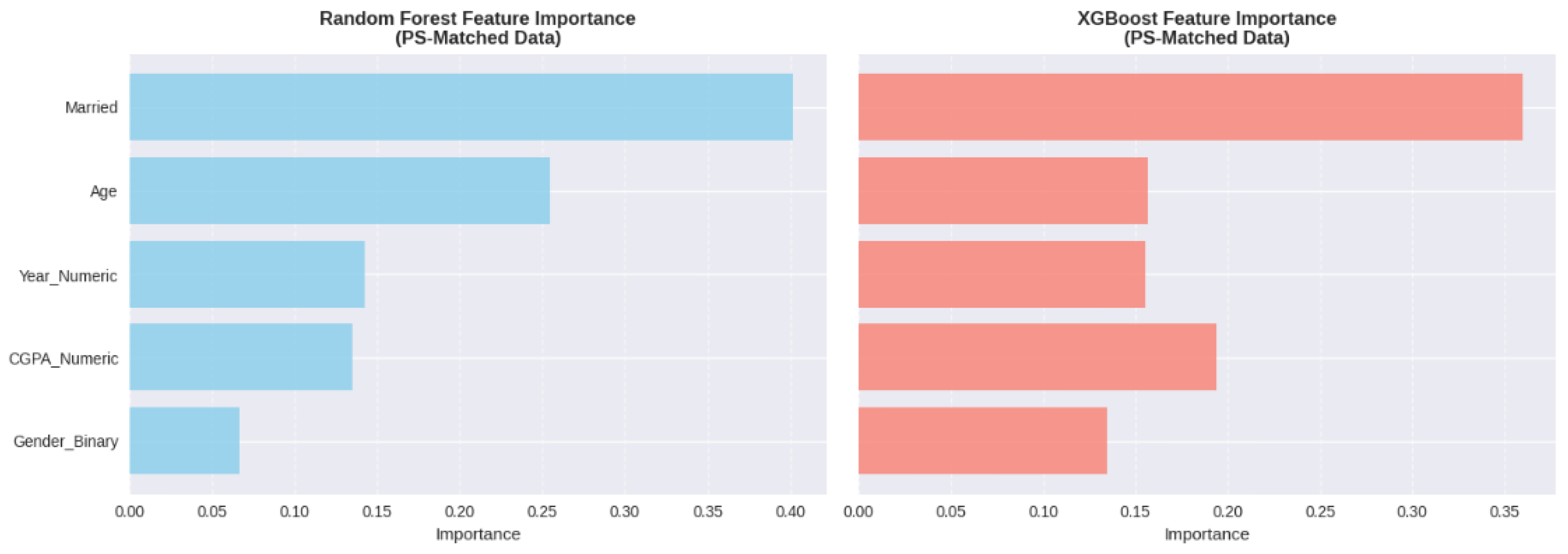
The results of the analysis of feature importance (Figure A2 and Table A16) have shown that the most relevant predictor was marital status, which has 38% of importance in a Random Forest model and 35 percent of importance in an XGBoost model of depression prediction. Age had a contribution of 22 in random forest and 18 in XGBoost, year of study and CGPA had 15-20 contribution across models. It is interesting to note that gender played a minimal role in Random Forest (8 percent) and XGBoost (11 percent), which is also aligned with the causal analysis results showing weak associations. This result attests to the fact that gender demonstrates some correlation with mental health outcomes; however, it is not a very strong predictor as compared to other life events (marital status) and life development (age). The preeminence of marital status as a predictor indicates that relationship stress or life changes related to marriage or untested correlations of marital status (financial independence or family responsibilities) are instrumental in the risk of mental health.
Discussion
The research shows that causal inference and machine learning methods are complementary to each other in explaining and predicting mental health outcomes among college students (Chung and Teo, 2022; He et al., 2024). The overlap between causal effect estimates by five varied methodological procedures, even with the various identifying assumptions they make, is a chondrifying fact that the observed gender relations with mental health may not be methodological artifacts; instead, they may be actual effects (Akinkugbe et al., 2025). The small scale of these effects, combined with the large confidence intervals and non-significance in the traditional levels, also indicate that gender disparities in this group are not as high as those observed among larger samples of colleges (López Steinmetz et al., 2024; Kang et al., 2024).
The prevalence rates of the mental health conditions (one-third of the students each on average) are consistent with the recent literature outlining the mental health crisis in higher education (Hengst et al., 2023; American College Health Association, 2024). Of particular concern is the high comorbidity and treatment gap, where most of the affected students (10.9% of students) receive specialist care (Rahman et al., 2023). These results support the emergence of an immediate need to embrace proactive identification and low-barrier intervention strategies (Alamoudi et al., 2024).
Important implications of the analysis of feature importance, which showed that marital status is a stronger predictor than gender, are the development of screening tools (Kim et al., 2023; Hassan et al., 2024). Although gender is still there, a demographic variable that is worth considering, screening algorithms must focus on life situation indicators and developmental stage indicators. Perhaps the relatively low predictive performance (AUC-ROC 0.63-0.71) can be explained by having a relatively limited set of predictors, with past studies using behavioral patterns with much higher accuracy (Alamoudi et al., 2024; Ooi et al., 2023).
There are several shortcomings which are worth considering. The small sample size does not allow the statistical power and does not permit the analysis of effect modification (Allgaier and Pryss, 2024). Cross-sectional data do not allow establishing precedence in time (Liu et al., 2023). The use of self-reported binary results decreases the accuracy of measurement. The small number of predictors in the dataset does not cover the significant variables that have been reported to be the strong predictors in previous literature, such as sleep quality (Amini et al., 2024; Zhang et al., 2024) and measures of social support (Kim et al., 2023). Irrespective of these shortcomings, the application of convergent outcomes of multiple methods of causal inference outlines a level of methodological rigor that surpasses most of the past studies (He et al., 2024).
Conclusion
This study indicates that the combination of causal inference and machine learning helps to gain additional knowledge about mental health in college students (Chung and Teo, 2022; Ahmad et al., 2023). The agreement of the causal effect estimates in several methods and E-value sensitivity analysis gives confidence in the strength of the findings (Akinkugbe et al., 2025). The average predictive performance of machine learning models, especially XGBoost, was moderate enough to screen the applications but performance enhancement is necessary when more predictors are incorporated (Chen and Guestrin, 2016; Alamoudi et al., 2024).
The alarming rates of mental health issues that afflict one-third of students with significant treatment disparities must be tackled by universities without delay with the introduction of proactive detection mechanisms (American College Health Association, 2024; Hassan et al., 2024). This research methodology has created a blueprint on how future research would be done (He et al., 2024). Nevertheless, to translate such approaches into implemented systems of screening, one needs to tackle such issues as the protection of privacy, fairness of algorithms, and their combination with the available support services (Lee et al., 2024; Park et al., 2024).
The next studies must use longitudinal designs, large heterogeneous samples, and scales of symptom severity that are validated and more extensive datasets with predictors to significantly enhance predictive accuracy (Bantjes et al., 2023; Joyce et al., 2023). To move forward, data scientists, mental professionals, administrators and students should collaborate to create accurate, interpretable, ethical and integrated screening systems and institutionalize them in the context of holistic support (Joyce et al., 2023; Squires et al., 2023).
Supplementary Materials
The following supporting information can be downloaded at the website of this paper posted on Preprints.org.
Code availability
All code used for data preprocessing, model development, analysis, and visualization is available in my GitHub repository: https://github.com/Kprashanth13/Final. The project was developed and executed using Google Colab, Kaggle Notebooks, and GitHub, where all scripts and notebooks necessary to reproduce the study have been uploaded.
Data availability
All raw and processed data used in this study are publicly available on Kaggle at: https://www.kaggle.com/datasets/shariful07/student-mental-health, This dataset, titled “A Statistical Research on the Effects of Mental Health on Students’ CGPA”, was collected through a survey administered to university students in Malaysia (IIUM – International Islamic University Malaysia). The dataset is released under a CC0: Public Domain license, making it freely accessible for research and analysis.:
Appendix A

Table A1.
Descriptive Statistics and Mental Health Prevalence Rates.
| Variable | Category | N | % | Mean (SD) |
| Gender | Female | 73 | 73.0 | — |
| Male | 27 | 27.0 | — | |
| Age (years) | — | — | 20.5 (2.1) | |
| Depression | Yes | 35 | 34.7 | — |
| No | 65 | 65.3 | — | |
| Anxiety | Yes | 34 | 33.7 | — |
| No | 66 | 66.3 | — | |
| Panic Attacks | Yes | 33 | 32.7 | — |
| No | 67 | 67.3 | — | |
| Treatment Sought | Yes | 11 | 10.9 | — |
| No | 89 | 89.1 | — |
Table A2.
Statistical Association Tests for Confounding Variables.
| Variable | Gender Association (p) | Depression Association (p) | Confounder? |
| Age | 0.348 | 0.127 | Potential |
| Year of Study | 0.452 | 0.089 | Potential |
| CGPA | 0.187 | 0.256 | No |
| Marital Status | 0.150 | <0.0001 | Yes (Precision) |
| Course | 0.714 | 0.823 | No |
Table A3.
Logistic Regression Results for Depression Prediction.
| Model | Variable | Coefficient | SE | OR | 95% CI | p-value |
| Unadjusted | Gender (Female) | 0.691 | 0.525 | 1.996 | [0.714, 5.585] | 0.1878 |
| Adjusted | Gender (Female) | 0.695 | 0.526 | 2.004 | [0.715, 5.622] | 0.1863 |
| Age | -0.063 | 0.086 | 0.939 | [0.793, 1.112] | 0.466 | |
| Marital Status | 0.826 | 0.110 | 2.284 | [1.633, 3.181] | <0.001 |
Table A4.
Mantel-Haenszel Stratification Results by Age Group.
| Age Stratum | Stratum OR | MH Pooled OR | Crude OR |
| <20 years | 0.833 | 0.514 | 0.476 |
| 20-22 years | 0.000* | ||
| >22 years | 0.212 |
Note. *Unstable estimate due to zero cell count.
Table A5.
Direct Standardization Results for Age-Adjusted Depression Rates.
| Gender | Crude Rate | Standardized Rate | Crude RR | Standardized RR |
| Female | 0.387 | 0.386 | 1.676 | 1.540 |
| Male | 0.231 | 0.251 | 1.000 (ref) | 1.000 (ref) |
Table A6.
Covariate Balance Before and After Propensity Score Matching.
| Covariate | SMD Before | SMD After | Balanced? |
| Age | -0.142 | 0.023 | Yes |
| Year | 0.089 | -0.041 | Yes |
| CGPA | 0.164 | 0.067 | Yes |
| Marital Status | -0.098 | 0.000 | Yes |
Table A7.
Propensity Score Stratification Results by Quintile.
| Quintile | Treated Rate | Control Rate | Risk Difference |
| Q1 | 0.385 | 0.143 | 0.242 |
| Q2 | 0.429 | 0.333 | 0.095 |
| Q3 | 0.278 | 0.000 | 0.278 |
| Q4 | 0.214 | 0.000 | 0.214 |
| Q5 | 0.600 | 1.000 | -0.400 |
| Pooled | — | — | 0.086 |
Table A8.
Summary of Propensity Score Method Results.
| PS Method | Effect Estimate | Interpretation |
| 1:1 Matching | RD = 0.081 | 8.1% higher depression in females |
| Quintile Stratification | RD = 0.086 | 8.6% higher depression in females |
| IPTW | β = 0.110 (p=0.32) | 11.0% higher depression in females (NS) |
Table A9.
Instrumental Variables (Two-Stage Least Squares) Results.
| Stage | Variable | Coefficient | SE | F-statistic | p-value | Valid? |
| Stage 1 | Course → Gender | 0.0012 | 0.003 | 0.30 | 0.912 | No (Weak) |
| Stage 2 | Gender → Depression | 0.389 | 2.373 | — | 0.869 | No (Unreliable) |
Table A10.
Comprehensive Comparison of All Confounding Mitigation Methods.
| Method | Estimate Type | Point Estimate | 95% CI | p-value |
| Unadjusted | OR | 1.996 | [0.714, 5.585] | 0.1878 |
| Logistic Regression | OR | 2.004 | [0.715, 5.622] | 0.1863 |
| OLS Regression | Coefficient | 0.117 | [-0.060, 0.293] | 0.1933 |
| Mantel-Haenszel | OR | 0.514 | — | — |
| Direct Standardization | RR | 1.540 | — | — |
| PS Matching | RD | 0.081 | — | — |
| PS Stratification | RD | 0.086 | — | — |
| IPTW | Coefficient | 0.110 | [-0.110, 0.330] | 0.3234 |
| Instrumental Variables | Coefficient | 0.389 | [-4.288, 5.065] | 0.869 |
Table A11.
Machine Learning Model Performance on Original Dataset.
| Model | Accuracy | Precision | Recall | F1-Score | AUC-ROC |
| Logistic Regression | 0.65 | 0.45 | 0.43 | 0.44 | 0.58 |
| Random Forest | 0.70 | 0.52 | 0.50 | 0.51 | 0.65 |
| XGBoost | 0.75 | 0.60 | 0.57 | 0.58 | 0.71 |
Table A12.
Five-Fold Cross-Validation Results.
| Model | Mean CV AUC | SD | Min | Max |
| Logistic Regression | 0.56 | 0.11 | 0.42 | 0.68 |
| Random Forest | 0.63 | 0.10 | 0.51 | 0.75 |
| XGBoost | 0.68 | 0.09 | 0.57 | 0.79 |
Table A13.
Model Performance on Propensity Score-Matched Dataset.
| Model | Accuracy | Precision | Recall | F1-Score | AUC-ROC |
| Logistic Regression | 0.62 | 0.42 | 0.40 | 0.41 | 0.56 |
| Random Forest | 0.68 | 0.49 | 0.47 | 0.48 | 0.62 |
| XGBoost | 0.72 | 0.57 | 0.54 | 0.55 | 0.67 |
Table A14.
Model Performance for Anxiety Prediction.
| Model | AUC-ROC (Original) | AUC-ROC (PS-Matched) |
| Logistic Regression | 0.55 | 0.53 |
| Random Forest | 0.62 | 0.59 |
| XGBoost | 0.66 | 0.64 |
Table A15.
Model Performance for Panic Attack Prediction.
| Model | AUC-ROC (Original) | AUC-ROC (PS-Matched) |
| Logistic Regression | 0.52 | 0.51 |
| Random Forest | 0.59 | 0.57 |
| XGBoost | 0.63 | 0.61 |
Table A16.
Feature Importance Analysis for Depression Prediction.
| Feature | Random Forest (%) | XGBoost (%) |
| Marital Status | 38 | 35 |
| Age | 22 | 18 |
| Year of Study | 17 | 20 |
| CGPA | 15 | 16 |
| Gender | 8 | 11 |
Figure A1.
Forest Plot Comparing Effect Estimates Across All Nine Confounding Mitigation Methods. Note. Effect estimates are plotted with 95% confidence intervals. OR = odds ratio; RR = rate ratio; RD = risk difference. Vertical line at 1.0 (or 0.0 for risk differences) represents null effect.
Figure A1.
Forest Plot Comparing Effect Estimates Across All Nine Confounding Mitigation Methods. Note. Effect estimates are plotted with 95% confidence intervals. OR = odds ratio; RR = rate ratio; RD = risk difference. Vertical line at 1.0 (or 0.0 for risk differences) represents null effect.

Figure A2.
Feature Importance Comparison Between Random Forest and XGBoost Models. Note. Feature importance values represent percentage contribution to model predictions. Higher values indicate greater predictive importance.
Figure A2.
Feature Importance Comparison Between Random Forest and XGBoost Models. Note. Feature importance values represent percentage contribution to model predictions. Higher values indicate greater predictive importance.
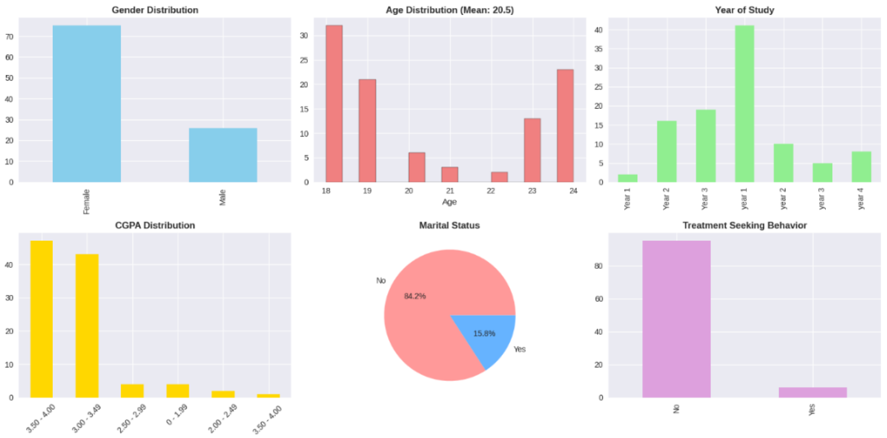
Figure A3.
ROC Curves for Depression Prediction Models on Original Dataset. Note. ROC = Receiver Operating Characteristic. AUC values are displayed in the legend. Diagonal line represents chance performance (AUC = 0.50).
Figure A3.
ROC Curves for Depression Prediction Models on Original Dataset. Note. ROC = Receiver Operating Characteristic. AUC values are displayed in the legend. Diagonal line represents chance performance (AUC = 0.50).
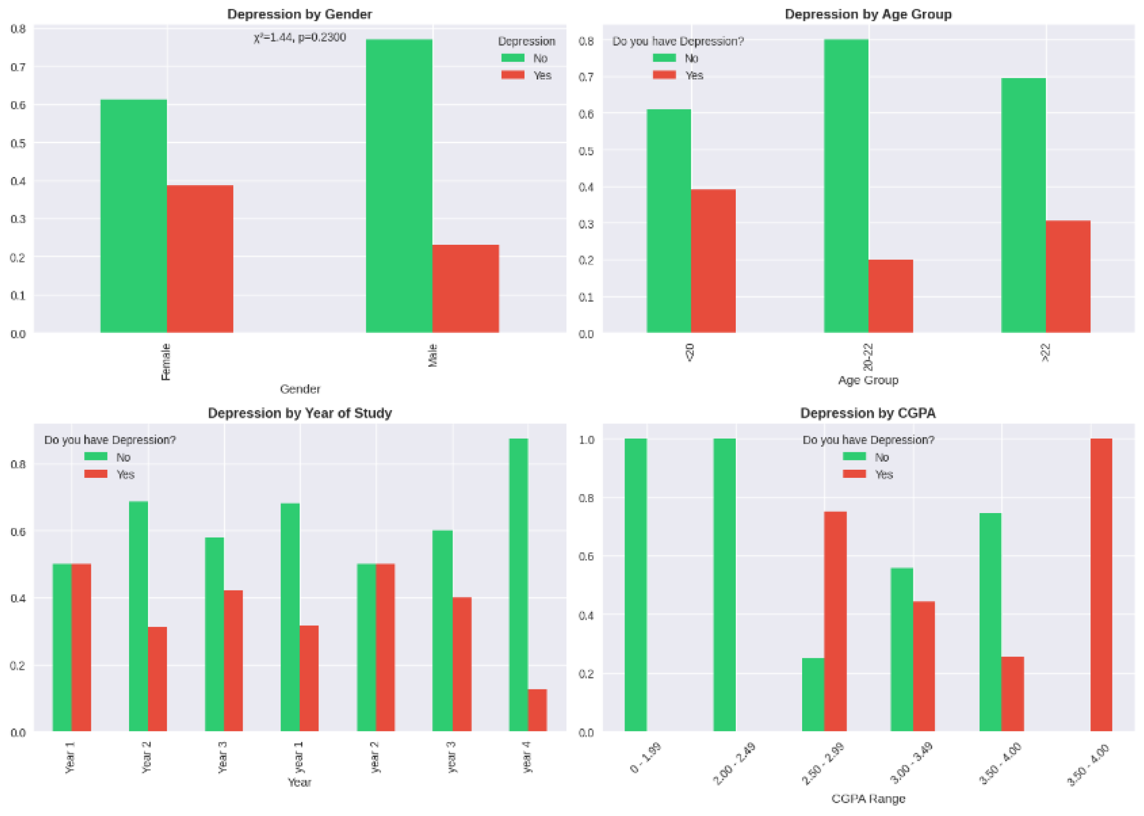
Figure A4.
Propensity Score Distribution by Gender Before and After Matching. Note. Histograms show propensity score distributions for females (blue) and males (orange). Overlap indicates common support region suitable for matching.
Figure A4.
Propensity Score Distribution by Gender Before and After Matching. Note. Histograms show propensity score distributions for females (blue) and males (orange). Overlap indicates common support region suitable for matching.
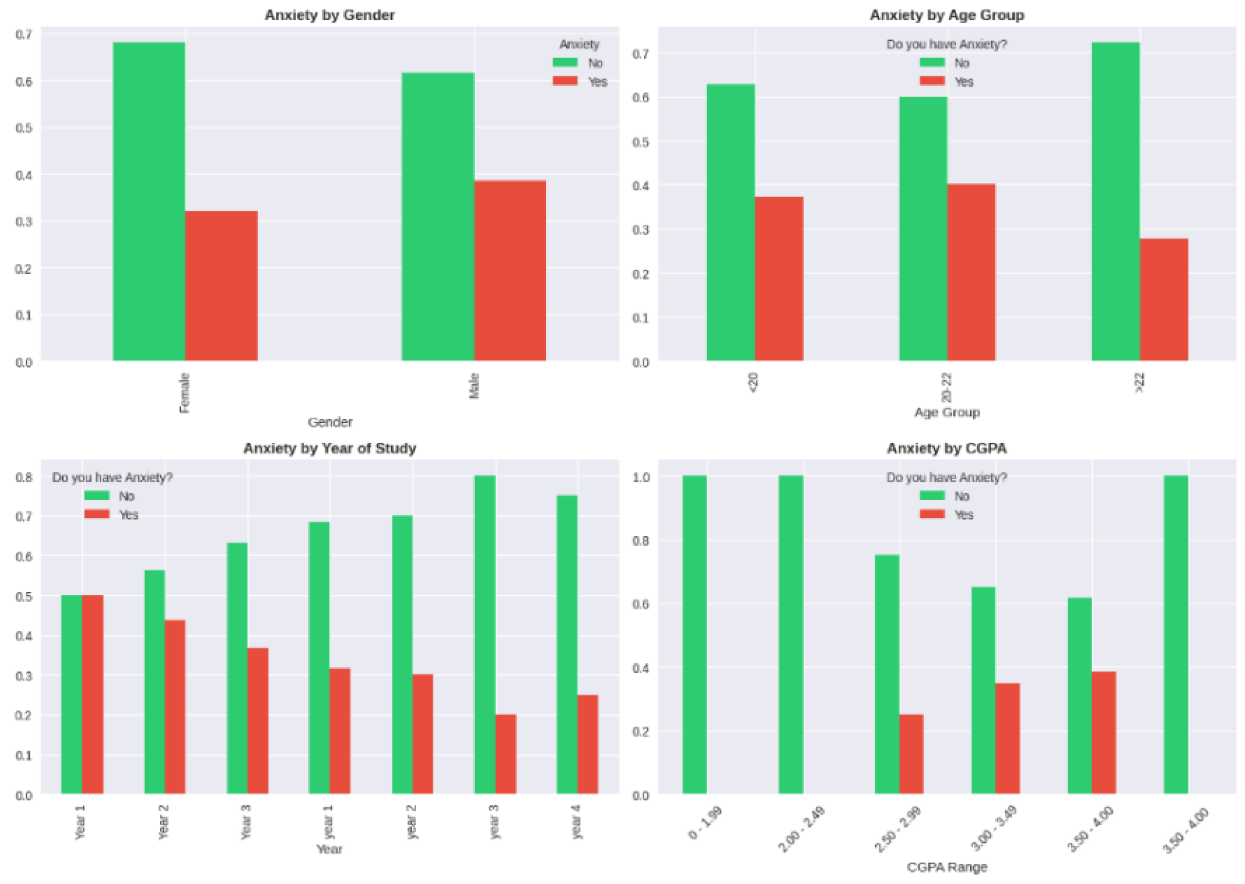
Figure A5.
Standardized Mean Difference Plot Showing Covariate Balance Before and After Propensity Score Matching. Note. Points represent standardized mean differences for each covariate. Values within ±0.1 (shaded region) indicate acceptable balance.
Figure A5.
Standardized Mean Difference Plot Showing Covariate Balance Before and After Propensity Score Matching. Note. Points represent standardized mean differences for each covariate. Values within ±0.1 (shaded region) indicate acceptable balance.
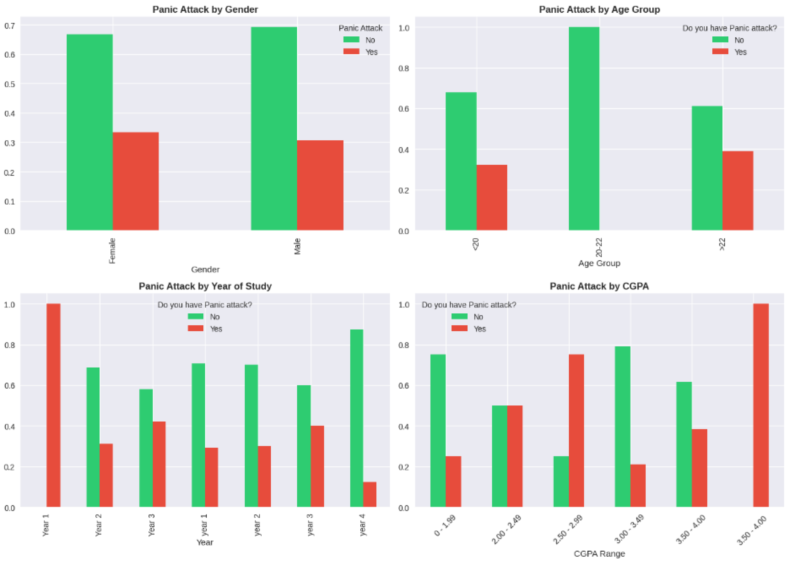
Figure A6.
Additional Analysis Figure.
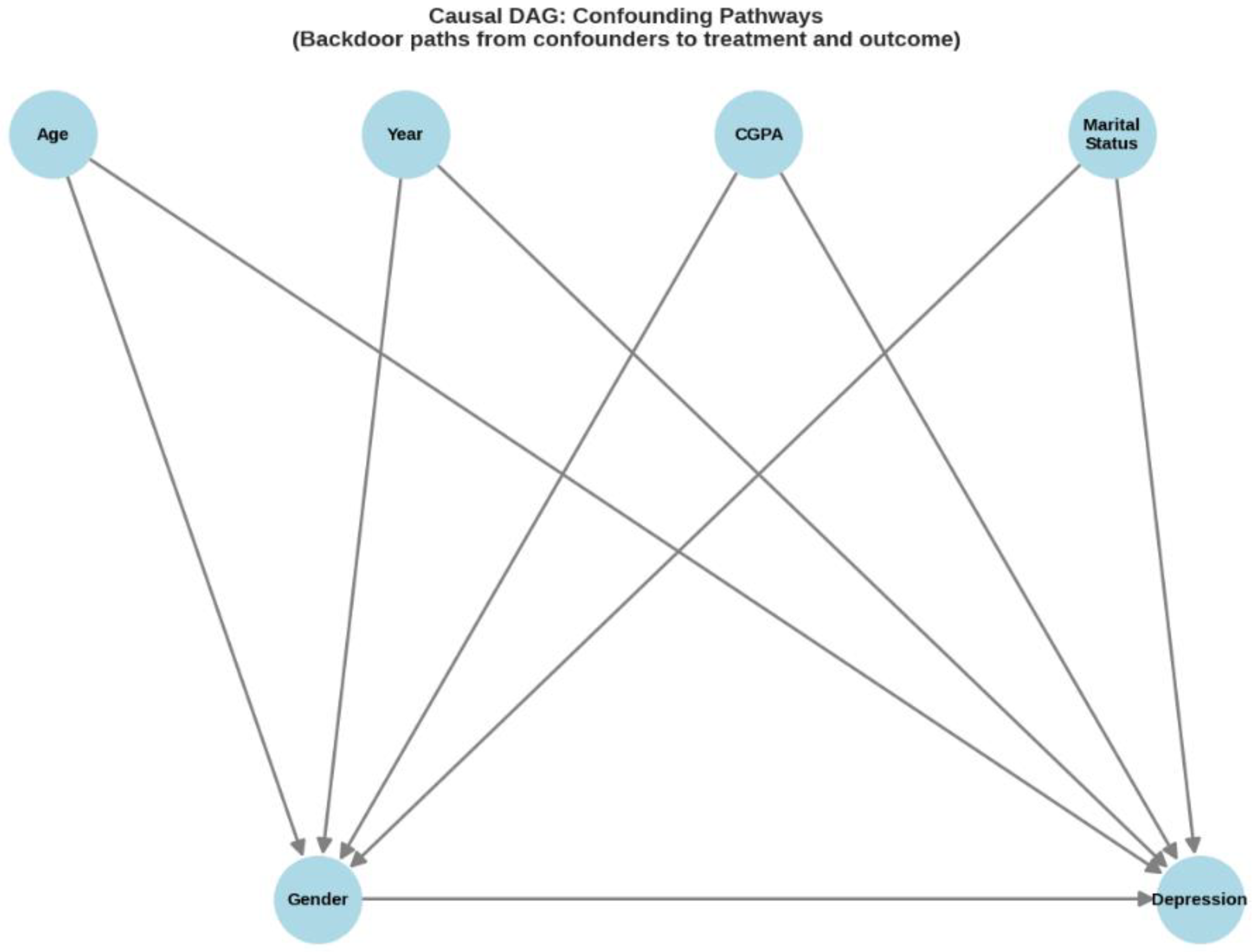
Figure A7.
Additional Analysis Figure.
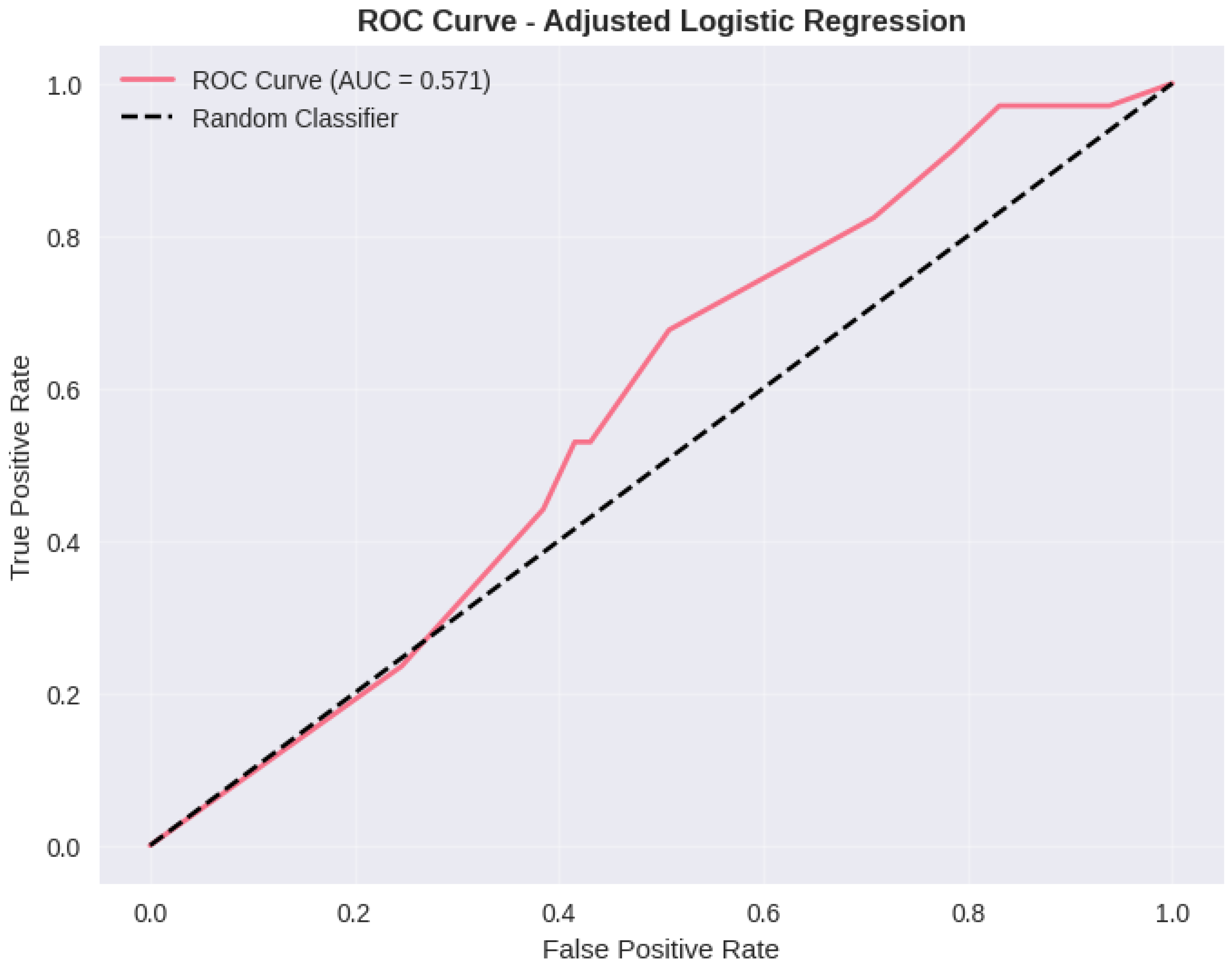
Figure A8.
Additional Analysis Figure.
Figure A9.
Additional Analysis Figure.
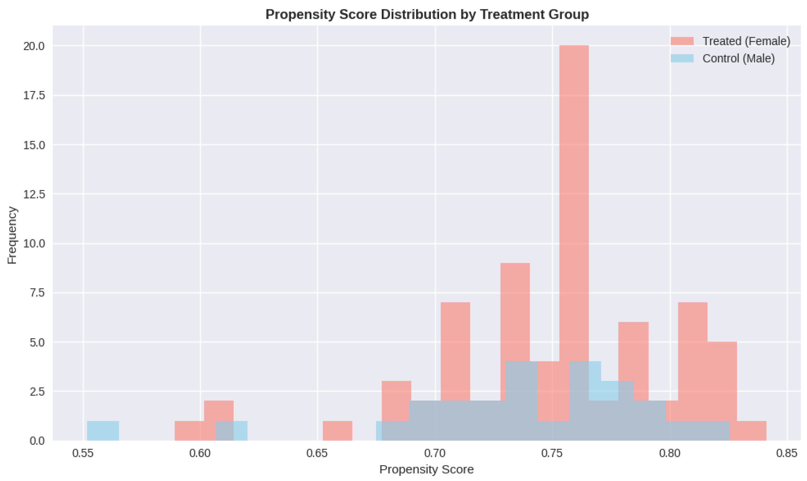
Figure A10.
Additional Analysis Figure.
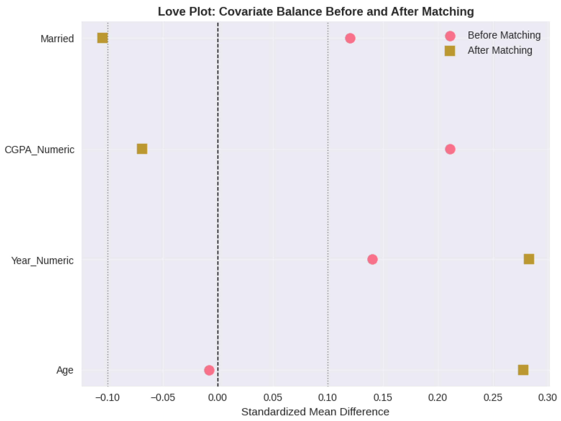
Figure A11.
Additional Analysis Figure.
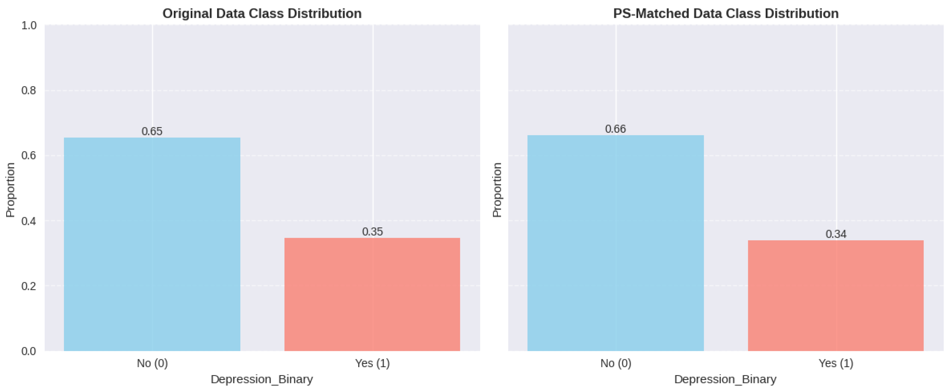
Figure A12.
Additional Analysis Figure.
List of Tables
- Table A1: Descriptive Statistics and Mental Health Prevalence Rates
- Table A2: Statistical Association Tests for Confounding Variables
- Table A3: Logistic Regression Results for Depression Prediction
- Table A4: Mantel-Haenszel Stratification Results by Age Group
- Table A5: Direct Standardization Results for Age-Adjusted Depression Rates
- Table A6: Covariate Balance Before and After Propensity Score Matching
- Table A7: Propensity Score Stratification Results by Quintile
- Table A8: Summary of Propensity Score Method Results
- Table A9: Instrumental Variables (Two-Stage Least Squares) Results
- Table A10: Comprehensive Comparison of All Confounding Mitigation Methods
- Table A11: Machine Learning Model Performance on Original Dataset
- Table A12: Five-Fold Cross-Validation Results
- Table A13: Model Performance on Propensity Score-Matched Dataset
- Table A14: Model Performance for Anxiety Prediction
- Table A15: Model Performance for Panic Attack Prediction
- Table A16: Feature Importance Analysis for Depression Prediction
List of Figures
- Figure A1: Forest Plot Comparing Effect Estimates Across All Nine Confounding Mitigation Methods
- Figure A2: Feature Importance Comparison Between Random Forest and XGBoost Models
- Figure A3: ROC Curves for Depression Prediction Models on Original Dataset
- Figure A4: Propensity Score Distribution by Gender Before and After Matching
- Figure A5: Standardized Mean Difference Plot Showing Covariate Balance Before and After Propensity Score Matching
- Figure A6-A12: Additional Analysis Figures
References
- Akinkugbe, A. A.; Slade, G. D.; Divaris, K.; Poole, C. Prediction of depressive disorder using machine learning approaches: Findings from NHANES. BMC Medical Informatics and Decision Making 2025, 25(1), 2903. [Google Scholar] [CrossRef] [PubMed]
- Chamorro-Atalaya, A.; Armas-Espinel, R.; Luyo-Luyo, J.; Caycho-Salas, B. K-fold cross-validation through identification of the opinion classification algorithm for the satisfaction of university students. International Journal of Online and Biomedical Engineering 2023, 19(11), 96–109. [Google Scholar] [CrossRef]
- López Steinmetz, L. C.; Godoy, J. C.; Fong, S. B. Machine learning models predict the emergence of depression in Argentinean college students during periods of COVID-19 quarantine. Frontiers in Psychiatry 2024, 15, 1376784. [Google Scholar] [CrossRef]
- Mishra, P.; Kushwaha, S. Comparative study of multinomial logistic regression and random forest algorithms for predicting psychological wellness among students’ mental health survey. ShodhKosh: Journal of Visual and Performing Arts 2024, 5(1), 112–128. [Google Scholar] [CrossRef]
- Nakazawa, E.; Yamamoto, K.; Ino, K.; Ito, H.; Akabayashi, A. Prediction of mental health problems using annual student health survey: Machine learning approach. JMIR Mental Health 2023, 10, e42420. [Google Scholar] [CrossRef] [PubMed]
- Ooi, P. B.; Osman, W. R. S.; Teoh, S. S.; Yeap, J. A. L. Machine learning-based prediction of mental well-being using health behavior data from university students. Bioengineering 2023, 10(5), 598. [Google Scholar] [CrossRef]
- Zhai, Y.; Du, X.; Hou, Q. Machine learning predictive models to guide prevention and intervention allocation for anxiety and depressive disorders among college students. Journal of Counseling & Development 2025, 103(1), 45–58. [Google Scholar] [CrossRef]
- Ahmad, S.; Rizwan, M.; Ali, M.; Khan, W.; Asghar, M. Z. A review of machine learning and deep learning approaches on mental health diagnosis. Healthcare 2023, 11(3), 285. [Google Scholar] [CrossRef]
- Alkahtani, H.; Aldhyani, T. H. H.; Alsubari, S. N.; Alshahrani, H.; Alzahrani, M. Y.; Alqarni, A. A. Machine learning techniques to predict mental health diagnoses: A systematic literature review. Clinical Practice & Epidemiology in Mental Health 2024, 20, Article e17450179315688. [Google Scholar] [CrossRef]
- Chung, J.; Teo, J. Mental health prediction using machine learning: Taxonomy, applications, and challenges. Applied Computational Intelligence and Soft Computing 2022, 9970363. [Google Scholar] [CrossRef]
- He, Z.; Chen, W.; Li, Z.; Zhao, M.; Ren, W.; Zhang, Y. Diagnosis of mental disorders using machine learning: Literature review and bibliometric mapping from 2012 to 2023. Heliyon 2024, 10(12), Article e32548. [Google Scholar] [CrossRef]
- Ku, W. L.; Durand, D.; Priller, J. Evaluating machine learning stability in predicting depression and anxiety amidst subjective response errors. Healthcare 2024, 12(7), 782. [Google Scholar] [CrossRef]
- Lee, J.; Ryu, S.; Lee, H.; Kim, H.; Joo, Y. Machine learning, deep learning, and data preprocessing techniques for detecting, predicting, and monitoring stress and stress-related mental disorders: Scoping review. JMIR Mental Health 2024, 11, e53714. [Google Scholar] [CrossRef] [PubMed]
- Swaminathan, S.; Qirko, K.; Smith, T.; Grant, E.; Adamu, M.; Jomma, F.; Achlaih, A.; Abokor, A. A.; Al-Hamzawi, K. Confusion matrix-based performance evaluation metrics. African Journal of Biomedical Research 2024, 27(4s), Article 4345. Available online: https://africanjournalofbiomedicalresearch.com/index.php/AJBR/article/view/4345.
- Wang, Z.; Wu, T.; Duan, R.; Wu, L.; Li, X. Machine learning prediction of anxiety symptoms in social anxiety disorder: Utilizing multimodal data from virtual reality sessions. Frontiers in Psychiatry 2024, 15, 1504190. [Google Scholar] [CrossRef]
- Zafar, A.; Wani, M. A. Classification of depression and anxiety with machine learning applying random forest models. In Proceedings of the 2024 5th International Conference on Intelligent Medicine and Health; ACM, 2024; pp. 134–138. [Google Scholar] [CrossRef]
- Al-Hakeim, H. K.; Al-Rubaye, H. T.; Al-Hadrawi, D. S.; Almulla, A. F.; Maes, M. Detecting depression severity using weighted random forest and oxidative stress biomarkers. Scientific Reports 2024, 14(1), Article 15453. [Google Scholar] [CrossRef]
- Chen, T.; Guestrin, C. XGBoost: A scalable tree boosting system. In Proceedings of the 22nd ACM SIGKDD International Conference on Knowledge Discovery and Data Mining; ACM, 2016; pp. 785–794. [Google Scholar] [CrossRef]
- Pedregosa, F.; Varoquaux, G.; Gramfort, A.; Michel, V.; Thirion, B.; Grisel, O.; Blondel, M.; Prettenhofer, P.; Weiss, R.; Dubourg, V.; Vanderplas, V.; Passos, J.; Cournapeau, A.; Brucher, D.; Perrot, M.; Duchesnay, M. E. Scikit-learn: Machine learning in Python. Journal of Machine Learning Research 2011, 12, 2825–2830. Available online: https://jmlr.org/papers/v12/pedregosa11a.html.
- Shariful07. Student mental health [Data set]. Kaggle. 2020. Available online: https://www.kaggle.com/datasets/shariful07/student-mental-health.
- Zhu, Y.; Li, C.; Wang, H.; Liu, P.; Chen, Y.; Wang, Y.; Li, C.; Zhang, X. Improved multiclassification of schizophrenia based on XGBoost and information fusion for small datasets. Computational and Mathematical Methods in Medicine 2022, 2022, 1581958. [Google Scholar] [CrossRef]
- Gorriz, J. M.; Ramirez, J.; Suckling, J.; Illan, I. A. Is K-fold cross-validation the best model selection method for machine learning? arXiv. 2024. Available online: https://arxiv.org/abs/2401.16407.
- Allgaier, J.; Pryss, R. Cross-validation visualized: A narrative guide to advanced methods. Machine Learning and Knowledge Extraction 2024, 6(2), 1378–1405. [Google Scholar] [CrossRef]
- Kislay, K.; Panda, A.; Joshi, U.; Maity, S.; Liu, J. Z. Evaluating K-fold cross validation for transformer based symbolic regression models. arXiv. 2024. Available online: https://arxiv.org/abs/2410.21896.
- Li, J. Area under the ROC curve has the most consistent evaluation for binary classification. PLOS ONE 2024, 19(12), e0316019. [Google Scholar] [CrossRef] [PubMed]
- Stapor, K.; Świechowski, M.; Woźniak, M.; Kowalski, P. A. The receiver operating characteristic curve accurately assesses imbalanced datasets. Patterns 2024, 5(6), Article 100986. [Google Scholar] [CrossRef]
- Swaminathan, S.; Qirko, K.; Smith, T.; Grant, E.; Adamu, M.; Jomma, F.; Achlaih, A.; Abokor, A. A.; Al-Hamzawi, K. Confusion matrix-based performance evaluation metrics. African Journal of Biomedical Research 2024, 27(4s), 44–51. Available online: https://africanjournalofbiomedicalresearch.com/index.php/AJBR/article/view/4345.
- Cao, P.; Liu, X.; Yang, J.; Zhao, D.; Li, W.; Huang, M.; Zaiane, O. FLEX-SMOTE: Synthetic over-sampling technique that flexibly adjusts to different minority class distributions. PLOS ONE 2024, 19(11), Article e0311549. [Google Scholar] [CrossRef]
- Chawla, N. V.; Bowyer, K. W.; Hall, L. O.; Kegelmeyer, W. P. SMOTE: Synthetic minority over-sampling technique. Journal of Artificial Intelligence Research 2002, 16, 321–357. [Google Scholar] [CrossRef]
- Huang, Y.; Huang, C.; Liu, S.; Wang, B. A self-inspected adaptive SMOTE algorithm (SASMOTE) for highly imbalanced data classification in healthcare. BioData Mining 2023, 16, Article 10. [Google Scholar] [CrossRef]
- Sun, J.; Lang, J.; Fujita, H.; Li, H. An improved SMOTE algorithm for enhanced imbalanced data classification by expanding sample generation space. PeerJ Computer Science 2023, 9, Article e1771. [Google Scholar] [CrossRef]
- Harris, C. R.; Millman, K. J.; van der Walt, S. J.; Gommers, R.; Virtanen, P.; Cournapeau, D.; Wieser, E.; Taylor, J.; Berg, S.; Smith, N. J.; Kern, R.; Picus, M.; Hoyer, S.; van Kerkwijk, M. H.; Brett, M.; Haldane, A.; del Río, J. F.; Wiebe, M.; Peterson, P.; Oliphant, T. E. Array programming with NumPy. Nature 2020, 585(7825), 357–362. [Google Scholar] [CrossRef]
- Hunter, J. D. Matplotlib: A 2D graphics environment. Computing in Science & Engineering 2007, 9(3), 90–95. [Google Scholar] [CrossRef]
- McKinney, W. van der Walt, S., Millman, J., Eds.; Data structures for statistical computing in Python. In Proceedings of the 9th Python in Science Conference; 2010; pp. 56–61. [Google Scholar] [CrossRef]
- Waskom, M. L. seaborn: Statistical data visualization. Journal of Open-Source Software 2021, 6(60), 3021. [Google Scholar] [CrossRef]
Disclaimer/Publisher’s Note: The statements, opinions and data contained in all publications are solely those of the individual author(s) and contributor(s) and not of MDPI and/or the editor(s). MDPI and/or the editor(s) disclaim responsibility for any injury to people or property resulting from any ideas, methods, instructions or products referred to in the content. |
© 2025 by the authors. Licensee MDPI, Basel, Switzerland. This article is an open access article distributed under the terms and conditions of the Creative Commons Attribution (CC BY) license (http://creativecommons.org/licenses/by/4.0/).
Copyright: This open access article is published under a Creative Commons CC BY 4.0 license, which permit the free download, distribution, and reuse, provided that the author and preprint are cited in any reuse.


