Submitted:
28 November 2025
Posted:
01 December 2025
You are already at the latest version
Abstract
We propose a novel filtering framework based on phase-space that treats the error distribution as the marginal of a Wigner quasi-probability distribution and defines an effective uncertainty constant quantifying the minimal resolvable phase-space cell. Recognizing that observational updates systematically reduce uncertainty, we adopt a generalized Koopman-von Neumann equation grounded in operator dynamical modeling to propagate the density operator corresponding to the error distribution. The scaling parameter $\kappa$ quantifies the reduction in uncertainty following each filter update. Because the potential is retained only to second order, both propagation and update preserve Gaussian form, permitting direct application of Kalman recursion. Validated on 1215 orbits (LEO-GEO), the method shows that within a 3 min fit / 10 min forecast window observational noise contributes 350 m while unmodelled dynamics adds only 0.6 m. Kruskal-Wallis rank-sum tests and the accompanying scatter-plot trend rank semi-major axis as the dominant sensitive parameter. The proposed model outperforms Chebyshev and high-fidelity propagators in real time, offering a physically interpretable route for short-arc orbit prediction.
Keywords:
Koopman-von Neumann mechanics
; Kalman filtering
; adaptive dynamics
; Wigner phasespace distribution
; short-arc prediction
1. Introduction
Accurate and timely orbit prediction is essential for space situational awareness, collision avoidance, and satellite operations. As new objects continue to be launched, initial acquisition typically yields fewer than three minutes of short-arc data. These observations suffer from low signal-to-noise ratios, incomplete angular coverage, and insufficient arc length, rendering initial orbit determination (IOD) and subsequent propagation highly sensitive to both observational noise and dynamical model errors [1,2]. Traditional Bayesian sequential orbit determination assumes locally linearised dynamics, which can be insufficient when uncertainties are large and observations sparse. We therefore adopt a phase-space approach that capable retain the full nonlinear dynamics while naturally propagating both position and velocity uncertainties.
Phase-space methods offer a natural framework for describing the joint distribution of position and velocity errors. The Wigner quasi-probability distribution , originally introduced in quantum mechanics [3,4,5], provides a real-valued function on classical phase space that encodes both marginal uncertainties and their correlations in a single framework. Applications of the Wigner distribution beyond quantum mechanics, including time-frequency analysis in signal processing and stochastic control see Ref. [6,7,8,9,10]. The evolution of Wigner distribution under Hamiltonian dynamics is governed by the Von Neumann equation through the corresponding density operator. However, these formulations describe systems with fixed uncertainty structure, whereas successive filter updates systematically compress the error distribution and refine orbital knowledge. Recently, a generalized Koopman-von Neumann (KvN) equation has been derived within the Operational Dynamic Modeling framework [11], which establishes a unified quantum-classical mechanics by introducing a generalized algebra of observables. This formalism yields a continuously parametrised family of evolution equations, bridging the gap between diffusive, high-uncertainty dynamics and sharp, near-deterministic propagation. The generalised KvN equation, with its embedded scaling parameter , provides a single propagator that automatically adapts to varying uncertainty levels during orbit determination.
Existing orbit prediction methods employ distinct strategies for propagating state uncertainty. Polynomial extrapolation fits kinematic curves without reference to the underlying force model, which limits extrapolation accuracy beyond the observation span [12]. Deterministic propagators integrate the equations of motion but yield only point estimates, requiring separate methods for uncertainty quantification [13,14]. Kalman-type filters couple state estimation with covariance propagation through sequential prediction and update cycles. The extended Kalman filter linearises the dynamics at each time step via local Jacobian matrices [15,16], while the unscented Kalman filter propagates deterministically selected sigma points through the nonlinear dynamics to avoid explicit linearisation [17,18]. Both approaches, however, remain confined to Gaussian distributions and rely on successive local approximations of the propagated state. Particle filters avoid Gaussianity constraints by representing distributions as weighted particle ensembles, yet demand substantial computational resources when applied to high-dimensional orbital state spaces [19,20].
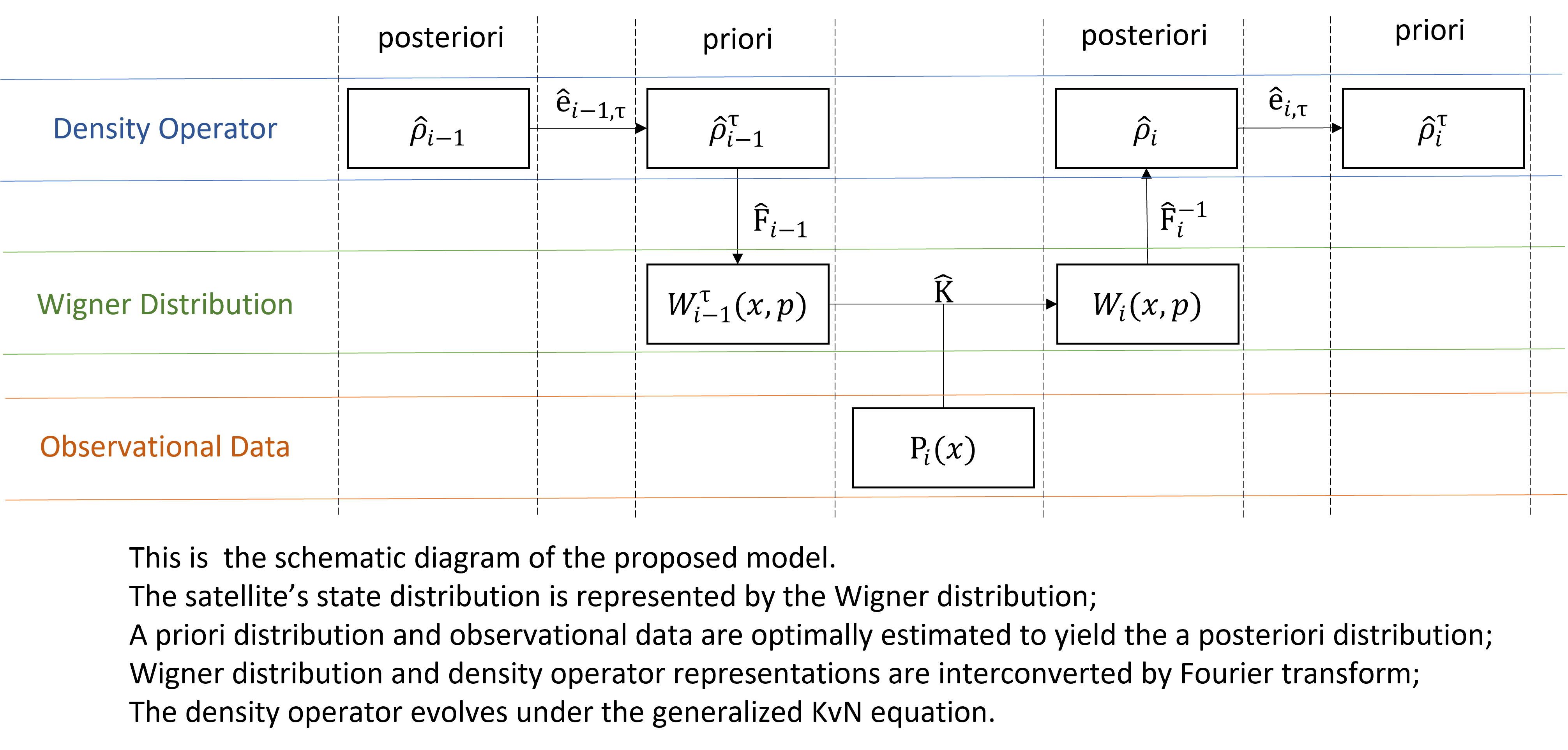
In this paper we propose a wigner-based Kalman filtering framework in which the observed position and velocity error distributions are treated as marginals of a Wigner quasi-probability distribution over classical phase-space, and we define an effective uncertainty constant that quantifies the minimal resolvable phase-space cell at each filter cycle. Because successive observations systematically compress the error distribution, refining orbital state knowledge, a propagator capable of accommodating continuously varying levels of uncertainty is required. To this end we adopt the generalized KvN equation that governs the temporal evolution of the density operator associated with the error distribution. The parameter parametrizes this transition: when observations are sparse, enforces a diffusive propagator consistent with high uncertainty; as measurements accumulate and posterior covariance contracts, asymtotically approaches zero and the propagator recovers the deterministic Liouville limit. At each prediction step the current density operator is propagated forward under this -scaled generalized KvN equation; the evolved density operator is then mapped back to its Wigner representation, which directly enters the filter update as the predicted error distribution. Under a second-order approximation of the gravitational potential, both propagation and update preserve Gaussian form, permitting direct application of Kalman recursion.
This formulation departs from conventional extended Kalman filtering by evolving the full phase-space density according to a global evolution equation rather than linearizing dynamics at successive state estimates, thereby retaining position-velocity correlations that arise from the coupled phase-space flow over the entire prediction horizon. The parameter is continuously adjusted based on the filter’s posterior covariance, enabling the propagator to transition smoothly from diffusive behavior under sparse observations to near-deterministic evolution as measurements accumulate. In the present implementation the gravitational potential is approximated to second order, preserving Gaussian form throughout the prediction-update cycle and reducing the scheme to an analytic Kalman recursion. This approach retains the computational tractability of Kalman filtering while incorporating richer dynamical information through global phase-space evolution. The theoretical framework nevertheless admits higher-order potentials and non-Gaussian error distributions, offering a natural pathway toward models that capture nonlinear perturbations.
To validate the method’s generality and quantify error sources, we design a comprehensive simulation campaign spanning 1 215 test cases. The parameter space covers three orbital regimes (Low Earth Orbit (LEO) at 400 km, Medium Earth Orbit (MEO) at 20 000 km, and Geostationary Orbit (GEO) at 35 786 km), two levels of dynamical fidelity, and two observational noise levels. Each case simulates a 3-minute observational arc followed by a 10-minute forecast horizon. Statistics show that within a 10-min forecast horizon the error is dominated by observational noise, whose contribution is two orders of magnitude larger than dynamical model error (500m vs.1.75m). Under identical 3-min arcs the -calibrated ODM consistently outperforms both Chebyshev-polynomial extrapolation and a high-fidelity dynamical propagator.
The remainder of this paper is organised as follows. In Section 2 we establishe the theoretical foundation of our Wigner-Kalman filtering framework, introducing the Wigner quasi-probability distribution, the KvN equation, the generalised KvN equation derived via the operator-dynamic model, and the resulting evolution equation for the Wigner distribution in phase space. Section 3 specifies the physical realisation of this framework for gravitational orbit dynamics, detailing the concrete form of the Wigner distribution appropriate for orbital states, the generalised KvN evolution under gravitational potentials and perturbative forces, the quantification of orbital uncertainty, and the calibration of the uncertainty parameter . Section 4 presents a comprehensive numerical validation through 1215 simulated orbital scenarios, analysing prediction accuracy across varying orbital regimes, observational noise levels, and filtering time windows. Section 5 summarises the principal findings, discusses current limitations, and outlines prospective extensions to multi-object tracking, non-Keplerian dynamics, and operational space situational awareness systems.
2. Wigner-Based Filtering Framework: Theoretical Foundation
This section establishes the mathematical foundation of our Wigner-based filtering approach by developing the operator-theoretic machinery necessary to represent and propagate probability distributions in phase space. Classical Kalman filtering characterises uncertainty via covariance matrices which is a representation that implicitly assumes Gaussian statistics and discards higher-order correlations. In contrast, our framework operates directly on the phase-space probability density , retaining the full structure of position-momentum correlations essential for accurate nonlinear orbit propagation.
We proceed in four stages. First, we introduce the Wigner quasi-probability distribution to characterise the error distribution in phase space, whose marginal distributions correspond to the experimentally measured position or velocity error distributions. We further define an effective uncertainty parameter based on the minimal resolvable volume element in phase space. Then, we review the Koopman-von Neumann formalism, which recasts classical Hamiltonian dynamics as unitary evolution on a Hilbert space of observables, providing a natural bridge between Liouvillian flow and operator-algebraic methods. The KvN formalism has gained renewed attention in recent years for data-driven modeling of complex dynamical systems, particularly in fluid dynamics and nonlinear control [21,22], and has been extended to non-Hamiltonian and dissipative systems through generalized formulations [23,24]. We further introduce the generalised KvN equation from operator-dynamic modeling, which features a continuous parameter that interpolates between broad (high-uncertainty) and sharply localised (low-uncertainty) phase-space distributions, and reformulate it to encode the filtering process as a geometric contraction in phase space. Finally, we present the concrete evolution scheme for the error Wigner quasi-probability distribution, wherein the Wigner function is propagated by evolving its associated density operator via the generalized KvN equation.
Taken together, this section constitutes a closed mathematical framework in which orbital filtering is realised through the continuous deformation of the Wigner distribution in phase space, driven by generalised Koopman-von Neumann dynamics and regulated by the -parameter that controls the transition from diffuse to localised probability densities. The physical realisation of this framework for gravitational systems is deferred to Section 3.
2.1. The Wigner Quasi-Probability Distribution
Classical mechanics represents the state of a deterministic system as a point in phase space, where denotes position and denotes momentum. When uncertainty enters through imperfect initial knowledge or observational noise, the natural generalisation is a probability density satisfying and . However, such classical phase-space distributions do not naturally accommodate the operator structure required for systematic uncertainty propagation via the Koopman-von Neumann formalism. The Wigner distribution, introduced by Wigner [25] in 1932, provides a phase-space representation that bridges classical probability densities and operator-algebraic methods [26,27,28,29]. Originally developed for quantum mechanics, the Wigner formalism has found broad applications in theoretical physics, signal processing, time-frequency analysis, and quantum information theory [6,8,30,31,32,33,34].
Consider a quantum-mechanical system with density operator on a Hilbert space . In the position representation, the Wigner function is defined via the Wigner–Weyl transform as
where denotes the position-space matrix element of the density operator. For a pure state , this reduces to
The Wigner formalism, though originally formulated for quantum systems, applies directly to classical phase-space dynamics. In the classical orbital setting, Equation (1) remains formally unchanged, but ℏ is reinterpreted as an effective parameter that quantifies the minimum resolvable phase-space volume element dictated by measurement errors rather than quantum indeterminacy. Here, serves as a phenomenological parameter encoding both observational precision and dynamical time scales relevant to the filtering problem. The Wigner distribution thereby captures the central orbital estimate via its peak location and the uncertainty spread via its width, analogous to a covariance matrix but retaining the full functional structure necessary for nonlinear dynamical evolution.
A defining property of the Wigner distribution is that its marginals recover the correct position and momentum probability densities:
where is the momentum-space wavefunction. Integrating out either variable yields the correct one-dimensional probability distribution, which is essential for filtering applications where observations typically measure only position (e.g., radar ranging) while velocity must be inferred through dynamical evolution. The full phase-space structure retains both observed and unobserved information consistently. A critical distinction between the Wigner distribution and classical probability densities is that can assume negative values in certain regions of phase space. This negativity does not violate physical principles because W is not directly observable; only its marginals and appropriately weighted integrals correspond to measurable quantities.
We now adapt this framework to orbital filtering. Two considerations motivate this choice. First, real tracking systems produce position estimates and velocity estimates with independent uncertainties whereas they evolve together through the equations of motion. A classical covariance matrix describes second-order statistics and linear correlations, but provides an incomplete representation when nonlinear dynamics induce non-Gaussian features or significant higher-order correlations. The Wigner distribution retains the full functional structure of the joint state, allowing more accurate propagation through nonlinear dynamics. Second, Equations (3)–(4) provide a direct link: given measured error distributions for position and for momentum, we can construct a Wigner function whose marginals exactly match the observations. The phase-space structure of W then captures how position and momentum uncertainties become correlated during propagation, even though the measurements themselves treat them separately.
In practice, orbital tracking systems deliver measurements whose errors are approximately Gaussian under typical conditions. The measured position distribution has the form
where denotes the estimated position and is the covariance matrix describing uncertainties along each spatial axis. For a diagonal , the determinant gives the overall error volume. The momentum distribution has a similar structure:
where is the estimated momentum (satellite mass m multiplied by observed velocity) and is the momentum covariance matrix with determinant . These Gaussian profiles arise from a combination of measurement noise, signal propagation effects, and receiver electronics.
To bridge these observed distributions with the Wigner formalism, we introduce an effective action parameter that quantifies the smallest phase-space volume resolvable given the measurement precision. The idea of defining an effective action from minimal phase-space cells also appears in Ref. [35] in a different physical context, though the explicit construction differs. We define characteristic uncertainties by taking geometric means:
which represent average widths of the error ellipsoids. We then set
This definition plays a dual role. On one hand, it ties the scale in the Wigner transform (Equation (1)) directly to measurable quantities and , removing any ambiguity about how to choose it. On the other hand, it identifies with the elementary phase-space cell volume , below which distinctions become meaningless given the available precision and relevant time scales.
With the observed Gaussian marginals (Equations (5) and (6)) in hand, we can write down the Wigner function of uncertainty distribution that reproduces them:
This function is positive everywhere, normalises to unity when integrated over all of phase space, and by construction reproduces Equations (5) and (6) when marginalized over or respectively. The factorised exponential reflects our assumption that position and momentum errors are uncorrelated at the moment of measurement. However, as evolves under the orbital dynamics, this factorisation typically breaks down and correlations emerge.
The key point is this: even though position and velocity are measured separately at any given time, their errors do not evolve independently between measurements. A straightforward classical approach that treats and as unrelated quantities will miss the correlations induced by the dynamics. The Wigner function encodes this coupling through its joint phase-space structure. Under generalised KvN equation (Section 2.4), W evolves according to the Hamiltonian flow, maintaining phase-space volume while letting correlations develop in a nonlinear fashion. Even when we start with a simple product state, evolution through nonlinear forces generally introduces cross-correlations that cannot be captured by propagating and separately.
It is instructive to note that Equation (9), though derived from observed error statistics, is fully compatible with the standard Wigner formalism based on density operators. The phase-space function can be inverted via Fourier transform,
to yield the density operator in position representation. Introducing two position coordinates , we obtain
Here and represent two independent position coordinates in the density operator representation, related to the phase-space coordinate and integration variable through and . Conversely, one can verify the consistency of this formalism by applying the forward Wigner transform to the density operator:
which recovers precisely the error distribution in Wigner form given by Equation (9). This closed-loop transformation confirms that our empirically motivated phase-space description is mathematically equivalent to a proper density operator, with serving as the effective quantization scale that bridges classical error statistics and phase-space distribution formalism.
Gaussian Wigner functions like Equation (9) provide natural initial conditions for orbital filtering and stay nearly Gaussian as long as nonlinearities remain weak. When nonlinear effects become significant, the Wigner approach offers a theoretical framework that can systematically handle these nonlinear influences, providing a potential pathway beyond linearised covariance methods. Overall, the Wigner quasi-probability distribution provides a phase-space representation that reproduces the classical position and momentum marginals to directly match the observed error statistics. It captures position–momentum correlations through its joint structure and a finite resolution scale determined from observations. Furthermore, it fits naturally into the Koopman-von Neumann operator framework, enabling a more systematic treatment of uncertainty propagation in nonlinear dynamics. The advantage of this framework lies in providing a systematic theoretical platform for handling coupled position-momentum uncertainties under nonlinear evolution.
2.2. The Koopman-von Neumann Formalism
The Koopman-von Neumann theory [36,37,38] provides an operator-algebraic formulation of classical mechanics that parallels the structure of quantum mechanics. Unlike the standard Hamiltonian formulation, which describes the trajectory of a point in phase space, the KvN formalism describes the evolution of a complex-valued wave function residing in a Hilbert space. This section reviews the essential elements of this formalism, which serves as the foundation for the generalized framework discussed later. Further details and applications of KvN theory can be found in Refs. [39,40,41,42].
Consider a one-dimensional classical system with position x and momentum p. The KvN formalism introduces four fundamental operators: , , , and , satisfying the commutation relations:
The key distinction from quantum mechanics is Equation (13): position and momentum commute, reflecting the classical nature of the underlying system. This ensures that position and momentum can be simultaneously measured with arbitrary precision, consistent with classical mechanics. The operators and are conjugate to and respectively and act as generators for translations in phase space.
According to Stone’s theorem on one-parameter unitary groups, the time evolution of the state vector is governed by a self-adjoint generator called the Liouvillian operator :
For a classical Hamiltonian system with Hamiltonian , the Liouvillian operator is constructed to reproduce the classical equations of motion. Following Ref. [11], a general form of the Liouvillian is:
where denotes the derivative of the potential and is an arbitrary real-valued function representing a gauge freedom. The first two terms generate the classical Hamiltonian flow in phase space. By computing the commutators and using the commutation relations (14)–(15), one can verify that the expectation values satisfy the Ehrenfest equations:
which have the form of classical Hamilton’s equations. Notably, the arbitrary function does not contribute to these equations, confirming its gauge nature.
To connect this framework with familiar classical descriptions, we project the formalism onto the -representation using the eigenstates . In this representation, the conjugate operators act as differential operators:
The wave function is given by , and substituting Equation (19) into the evolution Equation (16) yields:
The physically measurable quantity is the probability density in phase space:
Taking the time derivative of and using Equation (20), the contribution from the gauge function f cancels, yielding the classical Liouville equation:
where denotes the Poisson bracket. Thus, the KvN theory elegantly subsumes classical statistical mechanics as a natural consequence of operator dynamics in Hilbert space, providing the foundation for the -dependent generalization discussed next.
2.3. The Operator Dynamic Model and Generalised KvN Equation
Building upon the KvN formalism, Bondar et al. [3,11] developed a remarkable generalization that interpolates between classical and quantum mechanics through a continuous parameter . This section presents the mathematical structure of this framework, including the modified commutation relations, the unified Hamiltonian, and the limiting cases.
The generalization is achieved by replacing the commutation relation (13) with a -dependent version. Specifically, the operators and (where the subscript k indicates that these belong to the -dependent algebra) satisfy:
while the conjugate operators maintain their canonical commutation relations:
where and are the same operators as those in the KvN formalism.
We want the parameter continuously varies the fundamental uncertainty structure of the theory: when , Equation (23) recovers the classical commutation relation ; when , we obtain the canonical quantum commutation relation ; for , the system exhibits intermediate behavior with partial non-commutativity. This interpolation provides a one-parameter family of theories that smoothly connects classical and quantum descriptions. Based on the properties discussed above, one can derive the following two fundamental transformation formulas among these operators:
These transformation relations explicitly describe how the parameter mediates the coupling between the original operators and their modified counterparts through the conjugate momentum variables .
Following Ref. [11], the unified Hamiltonian operator for the -dependent system is constructed through consistency requirements known as the Ehrenfest conditions. These conditions demand that the time derivatives of the expectation values of position and momentum satisfy equations of the appropriate form. For a system with kinetic energy and potential energy , the unified Hamiltonian takes the form:
and the equation of motion is:
Under the -transformation the Hamiltonian can be written equivalently as:
To understand the structure of this Hamiltonian, consider the Taylor expansion of the potential terms for small :
Substituting into Equation (28) and keeping the leading terms, this reduces to:
which is precisely the classical Liouvillian (up to a factor of ℏ) discussed in Section 1.1.
Conversely, when , the commutation relation becomes the standard quantum relation . Substituting into Equation (26) and evaluating in the position representation yields:
This is the standard quantum Hamiltonian operator where function F is experimentally undetectable, confirming that the case reproduces quantum mechanics exactly.
For , the Hamiltonian defines a continuum of theories with partial non-commutativity. This intermediate regime is characterized by a generalized uncertainty relation that interpolates between the deterministic classical limit and the Heisenberg uncertainty principle. The physical interpretation of this regime and its application to orbital uncertainty propagation will be developed in Section 3. In the context of orbital mechanics, intermediate values of naturally describe systems with continuously decreasing uncertainty, providing a unified framework that smoothly connects deterministic trajectory propagation () with probabilistic descriptions ().
2.4. Evolution for the Wigner Quasi-Probability Distribution
The time evolution of the Wigner distribution can be approached in two distinct ways. The first is to evolve W directly via the Moyal equation, a nonlocal integro-differential equation in phase space. The second is to evolve the underlying density operator according to the generalised Koopman–von Neumann dynamics and then reconstruct via the Wigner transform at each time step. The present work adopts the latter approach.
This choice is motivated by the specific requirements of orbital filtering. In our framework, the effective uncertainty is initially determined from the measurement covariance and represents an intrinsic property of the observational system. However, each filtering cycle refines the state estimate and reduces the uncertainty in the error distribution. This manifests as a progressive narrowing of the distribution in phase space. In the ideal limit where all uncertainty is eliminated, the distribution would collapse to a delta function on phase space, corresponding to a state with simultaneously well-defined position and velocity. At that point, the evolution equation must reduce to the classical Liouville equation.
To accommodate this reduction in uncertainty at each filtering step, we introduce the parameter to quantify the degree of uncertainty present after each update. Correspondingly, the evolution equation itself must be adjusted to reflect the current level of uncertainty. This is precisely the role of the generalised Koopman–von Neumann framework: it interpolates continuously between the quantum-like regime (when and uncertainty matches ) and the classical limit (as ). Within this framework, evolving the density operator and then extracting the Wigner distribution is a natural and consistent procedure. It is worth noting that both approaches, direct Moyal evolution and density operator evolution, are theoretically equivalent, but the latter provides greater flexibility for handling the adaptive uncertainty parameter in the filtering context.
To extract the density operator elements from the generalized KvN equation and construct the evolution equation for the density operator, we transform the equation
that in the -representation to the -representation, where new variables introduced from
Under this transformation, the generalized KvN equation becomes
with the relation between functions in different representations given by
In operator form, this correspondence can be expressed as
where and denote position eigenstates in the extended Hilbert space, and represents the density operator. We introduce the modified position and momentum operators defined by
which act on the position eigenstates as multiplication and differentiation operators:
These operators form a canonical pair with the effective Planck constant , satisfying the commutation relation . The structure of Equation (34) can now be interpreted in terms of the commutator , where the effective Hamiltonian is given by
To establish this connection, we evaluate the matrix elements of the commutator in the position representation. The kinetic term yields
and the potential term gives
reflecting the difference in potential energy evaluated at the two positions. Combining these results, Equation (34) can be expressed in the compact operator form
which is recognized as the generalized von Neumann equation for the density operator evolution. This equation governs the dynamics of the -deformed density operator with serving as the effective uncertainty.
The formal solution over a time interval is
The numerical implementation of this evolution equation can be achieved through various computational approaches. In this work, we employ the split-step Fourier method, which provides an efficient and accurate scheme for time propagation of the density operator. Once the evolved density operator is obtained, we extract the corresponding Wigner distribution through the inverse transformation from the -representation. This allows us to compute the marginal distributions in position and momentum, which are then used in the filtering process to incorporate new measurement data.
At this stage, we have established a complete theoretical framework for the filtering procedure. It is worth emphasizing that our filtering approach is capable of handling arbitrary forms of error distributions and is not restricted to Gaussian cases, thus constituting a generalized Bayesian filtering method. However, for practical considerations and computational efficiency, we make a quadratic approximation to the gravitational potential experienced by the satellite orbit in subsequent numerical experiments. This approximation ensures that error distributions maintain their Gaussian character throughout the evolution process. Consequently, under the quadratic potential approximation, our filtering scheme reduces to a Kalman filter, which combines the computational advantages of linear-Gaussian systems with the theoretical generality of the extended phase space formalism.
3. Physical Realisation for Gravitational Orbit Dynamics
we now turn to the central question of this work: how to apply this framework to practical satellite orbit prediction. In this chapter, we address the implementation details within the specific context of short-arc satellite orbit prediction. The discussion encompasses several key aspects: first, we establish the procedure for selecting the covariance parameters and determining the effective uncertainty scale that characterizes the system; second, we specify the form of the Wigner distribution representing measurement errors in satellite state observations, taking into account the typical error characteristics in real tracking data; third, we derive the evolution equations appropriate for orbital motion under the extended phase space formalism and describe the numerical methods employed for their solution; finally, we present the complete filtering algorithm that integrates measurement updates with dynamical propagation and the parameter which determined adaptively through the filtering process based on the observed measurement uncertainties and state estimation errors, thereby enabling sequential state estimation for operational orbit determination scenarios.
3.1. Wigner Distribution for Orbital States
We begin by specifying the phase space representation of satellite states appropriate for optical tracking observations. In our experimental setup, ground-based optical stations measure the instantaneous range r and two angular coordinates (azimuth and elevation) that locate the satellite relative to the observation site. Through standard coordinate transformations from spherical to Cartesian coordinates, accounting for the station’s geodetic position and Earth’s rotation, these measurements yield the satellite’s three-dimensional position vector in an Earth-centered inertial frame. The measurement process involves multiple error sources including photon shot noise, atmospheric turbulence, timing uncertainties, and instrument calibration errors. A rigorous treatment of these contributions leads to an estimated position covariance matrix that characterizes the uncertainty in the reconstructed position.
For the velocity determination, we adopt a simplified model suitable for short-arc predictions where orbital perturbations remain small. Specifically, we assume the satellite follows a circular Keplerian orbit, for which the orbital speed satisfies
where G is the gravitational constant, M the Earth’s mass, and R the geocentric distance derived from the position measurement. The velocity vector (with m being the satellite mass) is then determined by imposing that it lies tangent to the instantaneous orbital plane and perpendicular to the position vector. The uncertainty in velocity propagates from the position measurement error through this relation.
In realistic orbital tracking, measurement uncertainties are rarely isotropic due to the geometry of ground stations, atmospheric effects, and instrumental biases. We therefore characterize the errors by covariance matrices and for position and momentum, which encode the magnitude and correlation structure of uncertainties. Under the assumption that errors follow Gaussian statistics, the Wigner function describing the satellite’s phase space distribution is given by
where and denote the mean position and momentum vectors derived from observations and dynamical models. The covariance matrices are typically obtained from orbit determination procedures that account for measurement noise and model uncertainties. This Gaussian form remains positive definite and represents the uncertainty compatible with the given error structure.
A crucial parameter in the extended phase space formalism developed in the previous chapter is the effective uncertainty scale , which plays the role of an effective Planck constant in the generalized quantum-like description. Following the convention established for Gaussian phase space distributions, we take the defination , which quantity quantifies the minimal resolvable volume element in phase space induced by measurement errors. It represents the fundamental cell size within which the satellite’s state cannot be further localized given the observational uncertainties. In other words, characterizes the coarse-graining scale of the phase space distribution imposed by the finite precision of tracking data, rather than arising from any fundamental quantum uncertainty relation. For typical low Earth orbit satellites with optical tracking precision on the order of meters to tens of meters and velocity uncertainties of millimeters per second (after accounting for the satellite mass), assumes values many orders of magnitude larger than Planck’s constant, reflecting the macroscopic nature of the system.
The Wigner distribution in Equation (45) can be mapped to the density operator representation in the phase space coordinates introduced in Chapter [previous chapter number]. Applying the inverse transformation from Wigner to density operator form yields
This representation serves as the initial state for the subsequent dynamical evolution and filtering procedure. The density operator in Equation (46) encodes both the mean orbital state and its associated uncertainty, providing the complete probabilistic description required for Bayesian inference in the orbit determination problem.
3.2. Generalised KvN Evolution under Gravitational Forces
In practical applications, we expand the potential energy around a reference point using a Taylor series. For the satellite orbit prediction problem considering Earth’s oblateness, the gravitational potential takes the form
where is the distance from Earth’s center, G denotes the gravitational constant, M represents the Earth’s mass, is the second zonal harmonic coefficient, km is the Earth’s equatorial radius, is the geocentric latitude with , and is the second-order Legendre polynomial.
We perform a second-order Taylor expansion about the reference position , which yields
where and is the Hessian matrix. This approximation remains valid when , making it suitable for short-arc orbit prediction scenarios.
Under the quadratic approximation of the potential, the generalised Hamiltonian simplifies to
where denotes the gradient of the potential function. In the representation, the evolution equation becomes
Transforming to the representation through the relations
the one-dimensional evolution equation takes the form
For three-dimensional systems with , this generalises to
The potential gradient required in the evolution equation is obtained by differentiating the second-order expansion:
Evaluating this at the positions and , and noting that the constant term drops out in the difference , the evolution equation becomes
The linear term in drives the center-of-mass motion of the wave packet, while the Hessian terms encode the local curvature of the gravitational field and govern the wave packet deformation.
To solve this evolution equation numerically, we employ the split-step Fourier method, which exploits the natural separation between kinetic and potential terms. The evolution equation can be recast in operator form as
where the kinetic operator is given by
and the potential operator takes the form
The formal solution over a time step is expressed as
Since the kinetic and potential operators do not commute, we apply a symmetric Trotter splitting to second-order accuracy:
The numerical implementation proceeds in five stages. First, we evolve the density operator by a half-step under the potential operator in real space:
where the effective potential is defined as
Second, we transform to momentum space via a six-dimensional Fourier transform:
Third, in momentum space the Laplacian operators become multiplicative, allowing us to apply a full kinetic evolution step:
Fourth, we return to real space through an inverse Fourier transform:
Finally, we complete the evolution with a second half-step under the potential operator:
The complete propagation scheme can be compactly written as
where and denote the forward and inverse Fourier transforms, respectively. This method preserves unitarity and maintains the trace of the density operator throughout the evolution, ensuring physically consistent results.
3.3. Flatering Procedure
After propagating the density operator over the time interval , the corresponding Wigner function is obtained through the Weyl transformation, from which the position marginal distribution follows by integration over momentum coordinates. Because the potential energy in our dynamical model retains only second-order terms in its Taylor expansion, the evolved Wigner distribution remains Gaussian in form, and consequently the position marginal distribution also preserves its Gaussian character. At the end of each propagation interval, a new observation of the satellite’s position becomes available. This fresh measurement, together with its associated covariance matrix, is then incorporated into the predicted position distribution via standard Kalman update equations. The filtering step combines the prior distribution (propagated density operator) with the observation likelihood, yielding a posterior distribution (filtered density operator) whose uncertainty is necessarily reduced relative to the prior. This updated distribution after propagation serves as the prior distribution for the next propagation interval, and this process is repeated each time a new observation is received.
Each Kalman update refines the state estimate by narrowing the error distribution, thereby progressively reducing the overall uncertainty of the error distribution. Since the posterior distribution at any given instant retains Gaussian form, it is fully characterized by the covariance matrices and . The variables and are defined by the following equations:
We define the rescaling parameter
The effective Planck constant for the posterior distribution is accordingly given by from Equation (68).
To make the filtering procedure explicit, we introduce discrete observation epochs , and separated by time intervals . Suppose the Kalman update at epoch has produced a filtered density operator and that posterior distribution is characterized by and . The rescaling parameter at this epoch is then
Over the interval , the density operator (cooresponds with posterior distribution) evolves according to
Integration over the interval yields the propagated density operator as well as the priori distribution just before the next measurement. At epoch , the new observation provides position and momentum data together with their covariance matrix. A standard Kalman update then combines this measurement with to produce the filtered density operator and the associated characters and of the posterior distribution. The updated rescaling parameter
governs propagation from to through the analogous equation
Repeating this propagation-update cycle for successive observations constitutes the complete filtering algorithm, wherein dynamical evolution and measurement assimilation alternate to maintain a statistically consistent representation of the satellite’s state under continuous observational input. The next section presents numerical results obtained with this procedure.
4. Experimental Results
4.1. Experimental Design and Data Generation
4.1.1. Orbit-Parameter Combinations and Simulation Setup
To comprehensively evaluate the proposed model, we simulate 405 satellite orbits by an almost exhaustive enumeration. The first five Keplerian elements are combined according to Table 1, and the mean anomaly is sampled at 30° intervals to guarantee full coverage of the station-visible orbital arcs.
4.1.2. Perturbation Modeling and Error-Source Characterization
The true trajectory is propagated for 13 min by Euler integration.
- Self-consistent run: only two-body plus J2 perturbation, identical to the force model used in the estimator.
- Biased run: additionally includes solar-radiation pressure and atmospheric drag to assess performance under small systematic errors.
Atmospheric-drag model:
where is the atmospheric density, the drag coefficient, A the cross-sectional area, and the velocity of the satellite relative to the atmosphere.
The perturbations are calculated according to Table 2, which gives their magnitudes relative to the Earth’s central two-body attraction.
4.1.3. Construction and Grouping Strategy of Observation Data
Each arc is split into an observation window (first 3 min) and a prediction window (subsequent 10 min). Three data sets are generated to quantify different error sources:
- (1)
- Clean (no-bias set): contains only machine-precision truncation errors; serves as the theoretical lower bound for filter consistency checks.
- (2)
- SysBias (small-bias set): adds un-modelled atmospheric drag and solar-radiation pressure (Table 2) to the true trajectory, yielding long-term drift at the level of ; used to test robustness under mild model mismatch.
- (3)
- ObsNoise (random-error set): further superimposes zero-mean Gaussian white noise on the SysBias truth, with standard deviations taken from current optical and laser ranging accuracies (radial , along/cross ); dominant in short-term scatter and used to evaluate the benefit of improving observation precision versus refining dynamical models.
4.2. Statistical Analysis of Prediction Errors
4.2.1. Ten-Minute Prediction-Error Distribution
Figure 1 presents the 10-minute position-error statistics (mean, median, trimmed mean and 1/4–3/4 quartile envelopes) for the three sample groups. The Clean group exhibits the smallest errors; the SysBias group shows a pronounced right tail; the ObsNoise group displays a distribution similar to that of the Clean group, indicating that observation precision is currently the dominant limiting factor.
4.2.2. Comparison Among Clean, SysBias and ObsNoise Groups
- Clean: errors grow linearly and slowly with time, confirming model self-consistency.
- SysBias: mean deviates from median, indicating systematic outliers.
- ObsNoise: envelope width increases markedly, yet without skewness; random errors dominate.
4.3. Parameter-Sensitivity Analysis
To further analyse the effects of bias and random errors on the prediction, we computed error distributions as functions of inclination, semi-major axis and eccentricity (Figure 2, Figure 3 and Figure 4) and identified inclination as an irrelevant variable. In the figures, “abs” denotes the absolute error, while R, T and N indicate the radial, transverse and normal components of the error, respectively.
4.3.1. Effect of Inclination (Verification of Irrelevance)
Figure 2 presents the error statistics grouped by inclination. Within each subset the distributions are virtually identical for all inclination values, confirming that inclination has no significant influence on prediction accuracy; this variable is therefore excluded from further analysis.
4.3.2. Coupled Effect of Semi-Major Axis and Perturbations
Figure 3 shows that for both the Clean and ObsNoise sets the error increases monotonically with the semi-major axis. In the SysBias set, however, a distinct peak appears at the smallest semi-major axis, corresponding to the maximum atmospheric-drag acceleration; at the largest semi-major axis the relative contribution of solar-radiation pressure rises, so the error induced by this perturbation also grows as the semi-major axis increases.
4.3.3. Modulation of Error Distribution by Eccentricity
Figure 4 indicates that only the SysBias set exhibits an increasingly pronounced outlier trend as eccentricity grows, whereas the distributions of the other two sets remain virtually unchanged with eccentricity.
4.3.4. Rank-Sum Sensitivity Test
To quantify, in a statistical sense, the influence of orbital parameters on forecast error, we applied the Kruskal-Wallis rank-sum test separately to inclination, semi-major axis and eccentricity. The null hypothesis is that the error rankings are identical across all factor levels; the method is a one-way non-parametric ANOVA that requires neither normality nor homoscedasticity, making it suitable for the highly non-Gaussian errors typical of short-arc orbit determination.
The test statistic is defined as
where k is the number of groups, the sample size of group i, the rank sum of group i, and the total number of observations. Under the null hypothesis H is approximately -distributed with degrees of freedom; the confidence (p-value) is obtained from , and is considered significant.
Table 3 summarise the H statistics and corresponding p-values for the four error components (abs, R, T, N) under the Clean, SysBias and ObsNoise scenarios. The main findings are as follows:
- Semi-major axis is highly significant for the abs error in all scenes (, H 350–840), confirming orbital altitude as the most sensitive parameter. The R component is also significant under SysBias (), while T is significant only in SysBias and N is never significant, indicating that altitude amplifies errors mainly within the orbital plane.
- Inclination shows only marginal significance for the R component in the Clean scene (); all other components and scenes yield with , verifying that inclination has no statistically significant influence on 10-minute forecast error.
- Eccentricity gives and H values 0.05–2.9 (far below ) in every scene and component, demonstrating that within the commonly used eccentricity range the short-term error is not significantly affected by this parameter.
Based on the rank-sum statistics, the parameter sensitivity ranking is: semi-major axis ≫ inclination ≈ eccentricity (non-significant).
4.4. Visualisation of Combined Bias and Error Effects
4.4.1. Scatter Plots of Radial / Along-Track / Cross-Track Errors
Figure 5 shows that the Clean-set scatter cloud is isotropic with the smallest spread. Figure 6 reveals that, under the action of systematic perturbations, the entire cloud of the SysBias set is shifted markedly in the radial and along-track directions; the combined effect of atmospheric-drag bias and large eccentricity further enlarges the cloud, while its spread in the cross-track direction increases as the actual orbital altitude decreases. Figure 7 displays a random, isotropic expansion of the scatter cloud for the ObsNoise set, with no directional offset.
4.4.2. Dominant-Factor Discrimination Between Bias and Noise
Comparing Figure 6 and Figure 7, the spread and directionality of the scatter clouds show that observational error enlarges the distribution range in all directions by at least a factor of 100. Consequently, for short-term prediction tasks with the present model, improving observation accuracy should take priority over refining the perturbation model.
4.4.3. Summary of Experimental Findings
In the typical 3-minute short-arc, 10-minute forecast scenario, error decomposition shows that observation noise contributes approximately 350 m, while unmodeled dynamical biases account for only 0.6 m—a three-order-of-magnitude difference. This indicates that the proposed model is sufficiently accurate for short-term prediction and demonstrates its robustness under information-deficient conditions: credible error bounds can still be obtained from observational data even when dynamical details are unknown. Statistical tests further show that inclination and eccentricity yield p>0.05 almost globally, implying no significant effect on error medians; however, boxplots and scatter diagrams reveal an increasing number of outliers as eccentricity grows.
5. Discussion
5.1. Comparison with Current Practice under SysBias
To benchmark our proposed model against current practice, we selected two widely-used methods—Chebyshev fitting and dynamical fitting—for comparison. We consider that the model-versus-truth errors of both approaches likewise fall under the SysBias category; hence we compare their results with those of the SysBias group in this paper.
Chebyshev polynomial extrapolation was tested with three fitting strategies [8,10], [10,18] and [14,30] (order, number of nodes). Table 4 shows that the best Chebyshev run ([10,18]) reaches 99.8 m at 20 sec forecast, while the proposed model achieves a median error of 1.75 m at 10 min (Figure 3(b)).
Dynamical extrapolation was performed with the Shanghai Astronomical Observatory EODP full-perturbation propagator. Table 5 gives 56.36 m (LEO) at 5 min and 56.45 m (GEO) at 10 min; the corresponding 10-min median errors of the proposed model are 1.75 m (LEO) and 0.00025 m (GEO) (Figure 3(b)), both substantially lower than the 5-min dynamical baseline.
Across the 3 min fit / 10 min forecast window, the proposed model achieves median errors of 1.75 m (LEO) and 0.00025 m (GEO), both substantially smaller than the 5 min baseline of the dynamical extrapolation tool and the 20 s best result of Chebyshev extrapolation, demonstrating clear accuracy gains under the same small-bias condition.
5.2. Future Improvements and Extensions
At present the model incorporates only conservative forces; for non-conservative effects such as atmospheric drag and solar-radiation pressure we have preliminarily introduced a forced-damped harmonic-oscillator equation. Initial experiments show that this correction reduces the 10-minute forecast error of the small-bias group by one to two orders of magnitude, providing a viable path for future accuracy improvements. In addition, we will test the model with pure angle-only (two-dimensional) data to verify its ability to handle incomplete observations and the stability of calibration under information-deficient conditions.
The proposed model presents an innovative approach to short-arc orbit prediction by integrating physical interpretability with real-time engineering feasibility. This approach not only enhances the accuracy and reliability of orbit predictions but also provides a robust framework for addressing the challenges associated with incomplete observations and uncertainties in dynamic environments. By effectively utilizing the principles of dynamics and leveraging observational data, this model demonstrates the potential to significantly advance the field of orbit prediction, ensuring improved performance in aerospace applications.
Author Contributions
Conceptualization, Qin Dong and Jinghui Zheng; methodology, Qin Dong; software, Qin Dong; validation, Qin Dong, Zhiyuan Chen and Jinghui Zheng; formal analysis, Qin Dong; investigation, Qin Dong and Juan Shi; data curation, Juan Shi; writing—original draft preparation, Qin Dong; writing—review and editing, Zhiyuan Chen and Jinghui Zheng; visualization, Qin Dong; supervision, Jinghui Zheng and Yindun Mao; project administration, Jinghui Zheng, Siyu Liu, Jingxi Liu. All authors have read and agreed to the published version of the manuscript.
Funding
This research was funded by National Key Laboratory of Space Target Awareness (No. STA2024ZCA0401).
Institutional Review Board Statement
Not applicable.
Informed Consent Statement
Not applicable.
Data Availability Statement
The data that support the findings of this study are openly available in ScienceDB at https://doi.org/10.57760/sciencedb.30894, reference number [10.57760/sciencedb.30894].
Acknowledgments
The Experimental Results and Discussion sections were originally written in Chinese and subsequently translated into English by Kimi (https://kimi.moonshot.cn, version 1.0, May 2025). All authors have reviewed and revised the AI-translated output and take full responsibility for the final content of this publication. All data and theoretical derivations presented in this paper are the original work of the authors and are released under CC BY 4.0.
Conflicts of Interest
The authors declare no conflicts of interest. The funders had no role in the design of the study; in the collection, analyses, or interpretation of data; in the writing of the manuscript; or in the decision to publish the results.
References
- Peng, H.; Bai, X. Improving orbit prediction accuracy through supervised machine learning. Advances in Space Research 2018, 61(10), 2628–2646. [Google Scholar] [CrossRef]
- Zhai, M.; Huang, Z.; Hu, Y.; Jiang, Y.; Li, H. Improvement of orbit prediction accuracy using extreme gradient boosting and principal component analysis. Open Astronomy 2022, 31, 229–243. [Google Scholar] [CrossRef]
- Bondar, D. I.; Cabrera, R.; Zhdanov, D. V.; Rabitz, H. A. Wigner phase-space distribution as a wave function. Physical Review A 2013, 88, 052108. [Google Scholar] [CrossRef]
- Kuz’menko, L. S.; Maksimov, S. G. Distribution functions in quantum mechanics and Wigner functions. Theoretical and Mathematical Physics 2002, 131, 641–650. [Google Scholar] [CrossRef]
- Polkovnikov, A. Phase space representation of quantum dynamics. Annals of Physics 2010, 325, 1790–1852. [Google Scholar] [CrossRef]
- Dragoman, D. Applications of the Wigner distribution function in signal processing. EURASIP Journal on Advances in Signal Processing 2005, 2005, 264967. [Google Scholar] [CrossRef]
- Najmi, A. H. The Wigner distribution: A time-frequency analysis tool. Johns Hopkins APL Technical Digest 1994, 15, 298–298. [Google Scholar]
- Hush, M. R.; Carvalho, A. R. R.; Hope, J. J. Number-phase Wigner representation for scalable stochastic simulations of controlled quantum systems. Physical Review A 2012, 85, 023607. [Google Scholar] [CrossRef]
- Ralph, J. F.; Maskell, S.; Ransom, M.; Ulbricht, H. Classical tracking for quantum trajectories. arXiv preprint arXiv:2202.00276 2022.
- Vladimirov, I. G.; Petersen, I. R.; James, M. R. A phase-space formulation and Gaussian approximation of the filtering problem for nonlinear quantum stochastic systems. Journal of Systems Science and Complexity 2017, 30, 279–298. [Google Scholar]
- Bondar, D. I.; Cabrera, R.; Lompay, R. R.; Ivanov, M. Yu.; Rabitz, H. A. Operational dynamic modeling transcending quantum and classical mechanics. Physical Review Letters 2012, 109, 190403. [Google Scholar] [CrossRef]
- Lin, Y.; Cheng, X.; Wang, Z.; Zhou, H. A Low Earth Orbit Satellite-Orbit Extrapolation Method. Aerospace 2024, 11, 746. [Google Scholar] [CrossRef]
- Sivasankar, P.; Lewis Jr, B. G.; Probe, A. B.; et al. A validation framework for orbit uncertainty propagation using real satellite data applied to orthogonal probability approximation. Acta Astronautica 2025, 232, 453–478. [Google Scholar] [CrossRef]
- Vallado, D. A.; Crawford, P. SGP4 Orbit Determination. AIAA/AAS Astrodynamics Specialist Conference 2008, AIAA 2008-6770.
- Tapley, B. D.; Schutz, B. E.; Born, G. H. Statistical Orbit Determination; Academic Press: Burlington, MA, USA, 2004. [Google Scholar]
- Kavitha, R.; Vathsal, S.; Desai, U. B. Extended Kalman filter-based precise orbit estimation of LEO satellites. IFAC-PapersOnLine 2022, 55, 54–59. [Google Scholar] [CrossRef]
- Julier, S. J.; Uhlmann, J. K. Unscented Filtering and Nonlinear Estimation. Proceedings of the IEEE 2004, 92, 401–422. [Google Scholar] [CrossRef]
- Pardal, P. C. P. M.; Kuga, H. K.; de Moraes, R. V. Analyzing the Unscented Kalman Filter Robustness for Satellite Orbit Determination. Journal of Aerospace Technology and Management 2013, 5, 29–38. [Google Scholar] [CrossRef]
- Mashiku, A. K.; Mathur, R.; Fitz-Coy, N. G. Statistical Orbit Determination using the Particle Filter for Incorporating Non-Gaussian Uncertainties. NASA Technical Report 2012. [Google Scholar]
- Cheng, Y.; Crassidis, J. L. Particle Filtering for Sequential Spacecraft Attitude Estimation. AIAA Guidance, Navigation, and Control Conference 2004, AIAA 2004-4855.
- Bevanda, P.; Sosnowski, S.; Hirche, S. Koopman operator dynamical models: Learning, analysis and control. Annual Reviews in Control 2021, 52, 197–212. [Google Scholar] [CrossRef]
- Joseph, I. Koopman–von Neumann approach to quantum simulation of nonlinear classical dynamics. Physical Review Research 2020, 2, 043102. [Google Scholar] [CrossRef]
- Bondar, D. I.; Gay-Balmaz, F.; Tronci, C. Koopman wavefunctions and classical–quantum correlation dynamics. Proceedings of the Royal Society A 2019, 475, 20180879. [Google Scholar] [CrossRef]
- Chruściński, D.; Jamiolkowski, A. Koopman’s approach to dissipation. Reports on Mathematical Physics 2006, 57, 319–331. [Google Scholar] [CrossRef]
- Wigner, E. On the quantum correction for thermodynamic equilibrium. Physical Review 1932, 40, 749–759. [Google Scholar] [CrossRef]
- Curtright, T. L.; Zachos, C. K. Quantum mechanics in phase space. Asia Pacific Physics Newsletter 2012, 01, 37. [Google Scholar] [CrossRef]
- Zurek, W. H. Decoherence, einselection, and the quantum origins of the classical. Nature 2003, 412, 712–719. [Google Scholar] [CrossRef] [PubMed]
- Dragoman, D.; Dragoman, M. Quantum-classical analogues; Springer: Berlin; New York, 2004; Chapter 8. [Google Scholar]
- Haroche, S.; Raimond, J. M. Exploring the quantum: atoms, cavities and photons; Oxford University Press: Oxford, 2006. [Google Scholar]
- Liu, T.; Ma, B.-Q. Quark Wigner distributions in a light-cone spectator model. Physical Review D 2015, 91(3), 034019. [Google Scholar] [CrossRef]
- Cohen, L. Time-frequency distributions—A review. Proceedings of the IEEE 1989, 77, 941–981. [Google Scholar] [CrossRef]
- Ferrie, C.; Emerson, J. Frame representations of quantum mechanics and the necessity of negativity in quasi-probability representations. New Journal of Physics 2009, 11, 063040. [Google Scholar] [CrossRef]
- Veitch, V.; Ferrie, C.; Gross, D.; Emerson, J. Negative quasi-probability as a resource for quantum computation. New Journal of Physics 2012, 14, 113011. [Google Scholar] [CrossRef]
- Mari, A.; Eisert, J. Positive Wigner functions render classical simulation of quantum computation efficient. Physical Review Letters 2012, 109, 230503. [Google Scholar] [CrossRef] [PubMed]
- Zurek, W. H. Sub-Planck structure in phase space and its relevance for quantum decoherence. Nature 2001, 412, 712–717. [Google Scholar] [CrossRef]
- Koopman, B. O. Hamiltonian systems and transformation in Hilbert space. Proceedings of the National Academy of Sciences 1931, 17, 315–318. [Google Scholar] [CrossRef]
- von Neumann, J. Zur Operatorenmethode in der klassischen Mechanik. Annals of Mathematics 1932, 33, 587–642. [Google Scholar] [CrossRef]
- von Neumann, J. Zusätze zur Arbeit “Zur Operatorenmethode...”. Annals of Mathematics 1932, 33, 789–791. [Google Scholar] [CrossRef]
- Gozzi, E.; Pagani, C. Universal local symmetries and nonsuperposition in classical mechanics. Physical Review Letters 2010, 105, 150604. [Google Scholar] [CrossRef] [PubMed]
- Brumer, P.; Gong, J. Born rule in quantum and classical mechanics. Physical Review A 2006, 73, 052109. [Google Scholar] [CrossRef]
- Carta, P.; Gozzi, E.; Mauro, D. Koopman–von Neumann formulation of classical Yang–Mills theories: I. Annalen der Physik 2006, 518, 177–215. [Google Scholar] [CrossRef]
- Blasone, M.; Jizba, P.; Kleinert, H. Path-integral approach to’t Hooft’s derivation of quantum physics from classical physics. Physical Review A 2005, 71, 052507. [Google Scholar] [CrossRef]
Figure 1.
Ten-minute prediction-error statistics. (a) Clean group; (b) SysBias group; (c) ObsNoise group.
Figure 1.
Ten-minute prediction-error statistics. (a) Clean group; (b) SysBias group; (c) ObsNoise group.
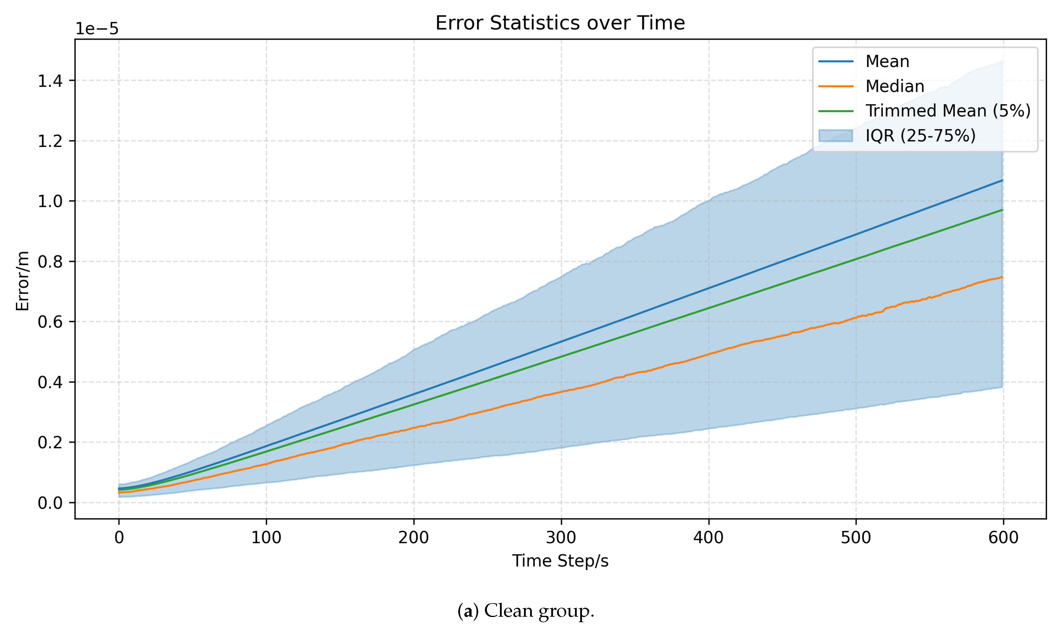
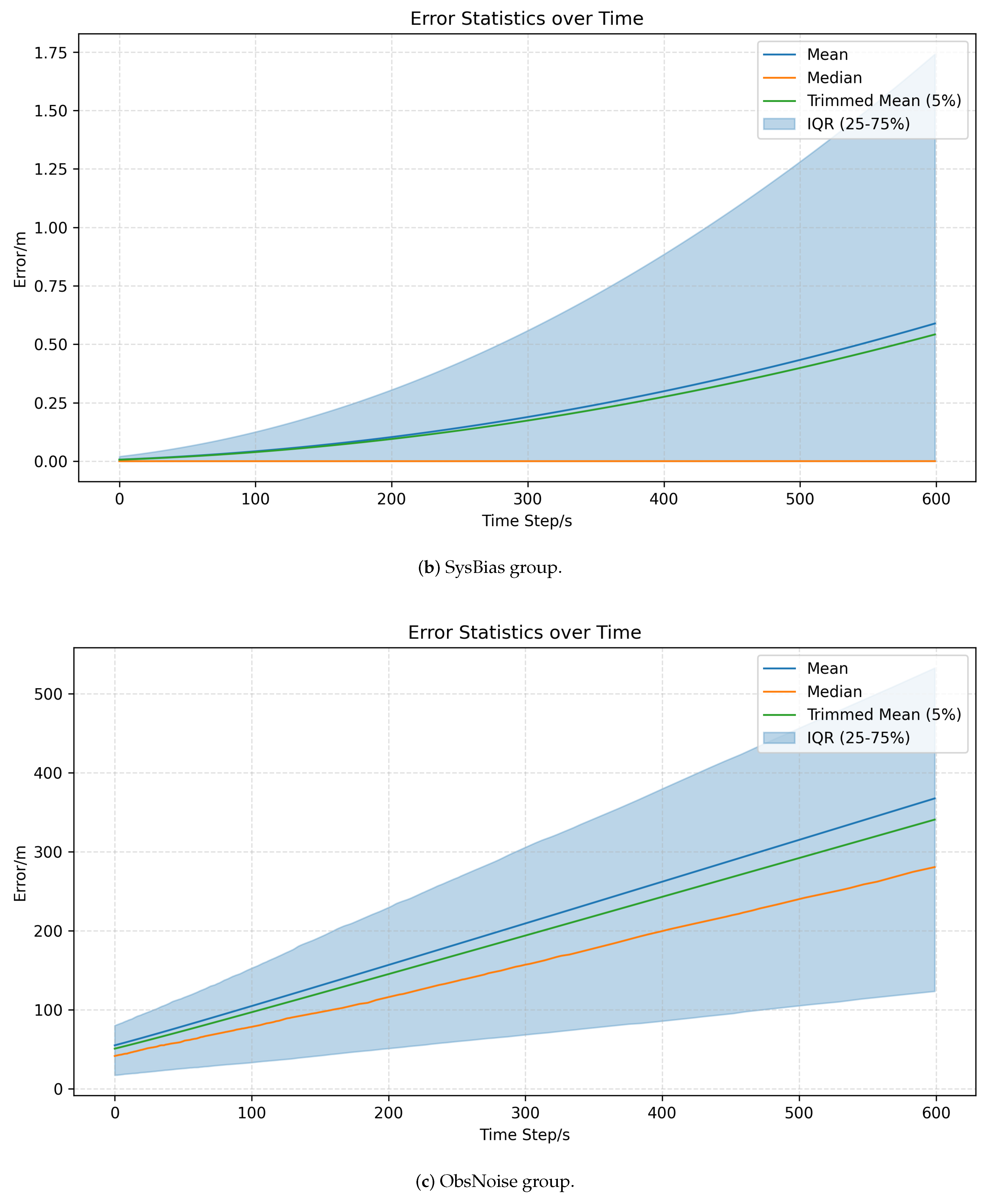
Figure 2.
Statistical Results Grouped by Inclination. (a) Clean group; (b) SysBias group; (c) ObsNoise group.
Figure 2.
Statistical Results Grouped by Inclination. (a) Clean group; (b) SysBias group; (c) ObsNoise group.
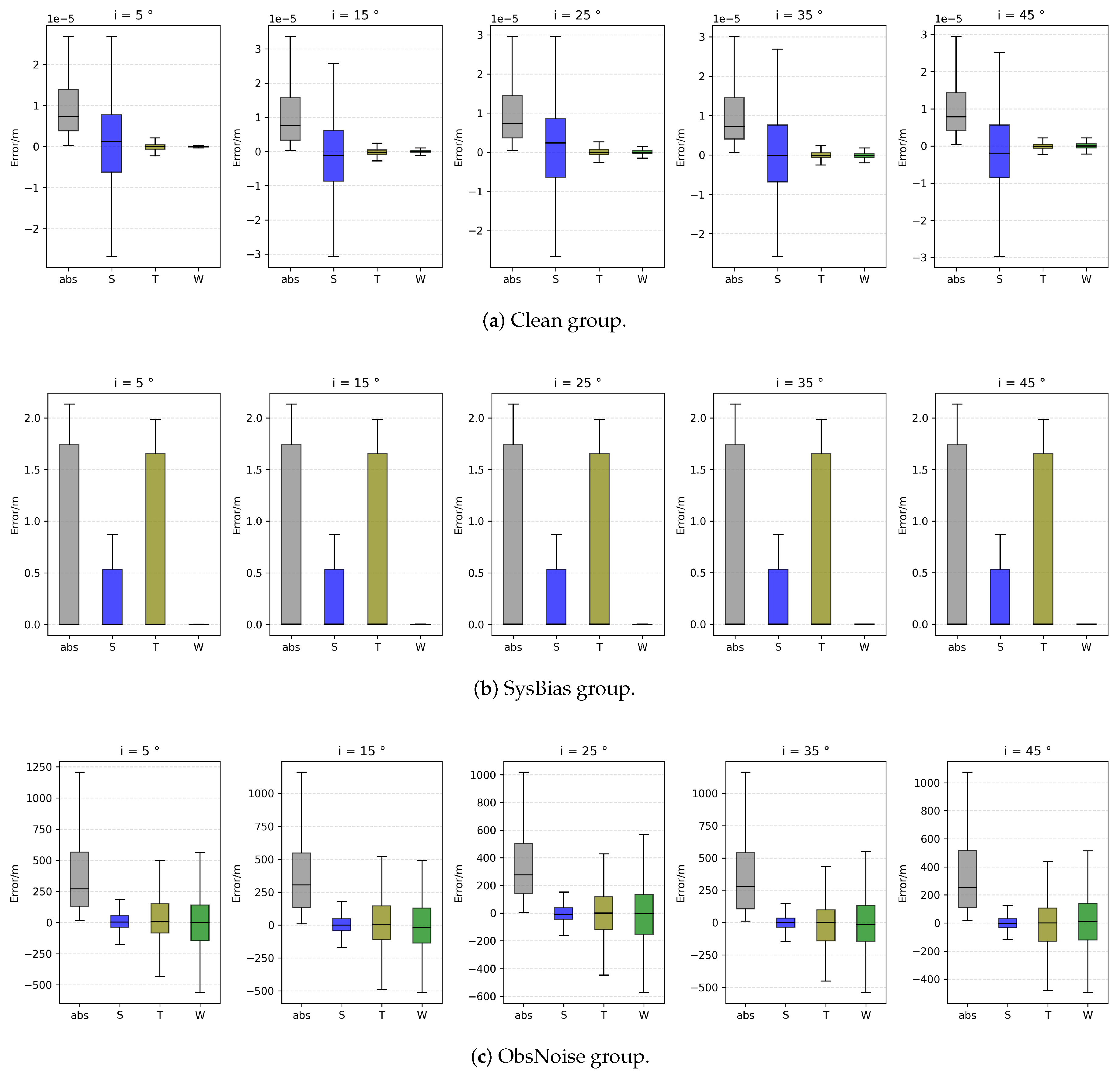
Figure 3.
Statistical Results Grouped by Semi-Major. (a) Clean group; (b) SysBias group; (c) ObsNoise group.
Figure 3.
Statistical Results Grouped by Semi-Major. (a) Clean group; (b) SysBias group; (c) ObsNoise group.
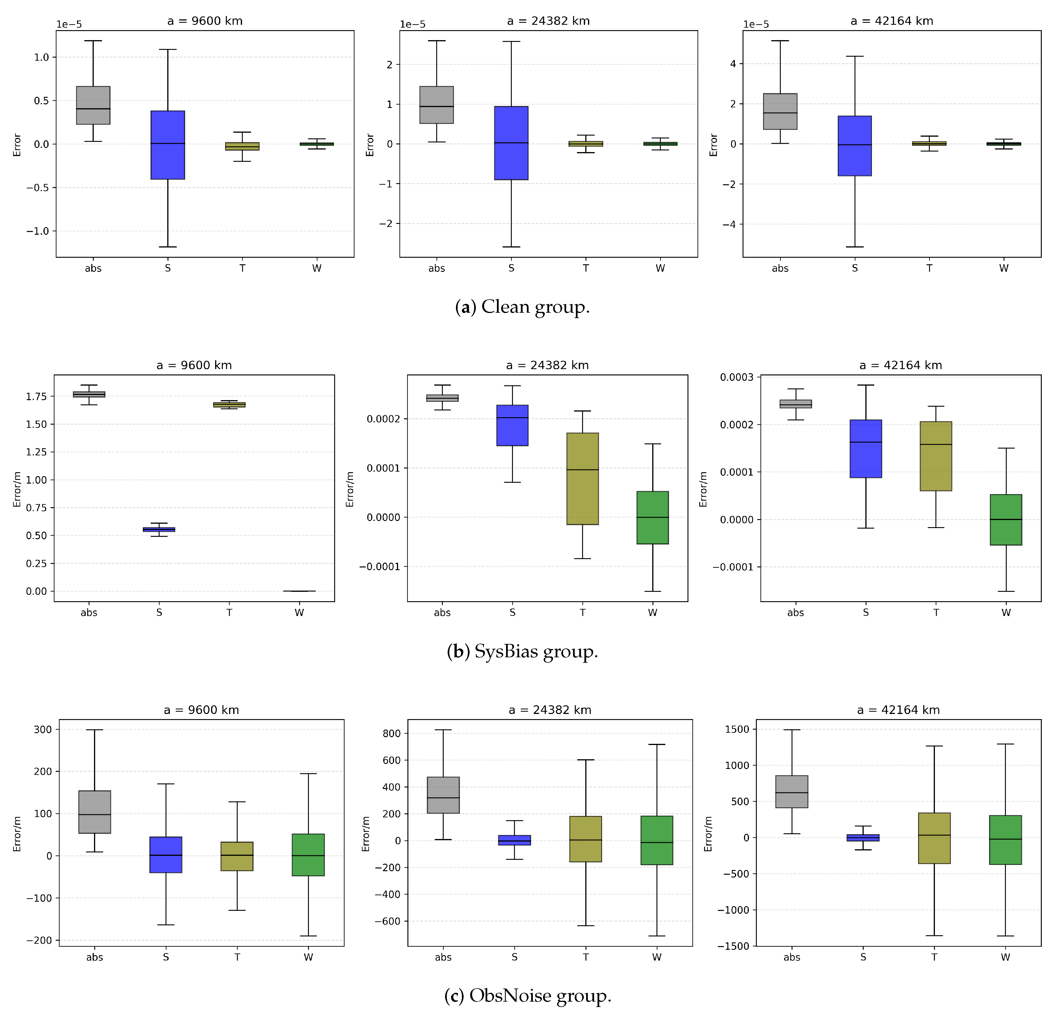
Figure 4.
Statistical Results Grouped by Eccentricity. (a) Clean group; (b) SysBias group; (c) ObsNoise group.
Figure 4.
Statistical Results Grouped by Eccentricity. (a) Clean group; (b) SysBias group; (c) ObsNoise group.
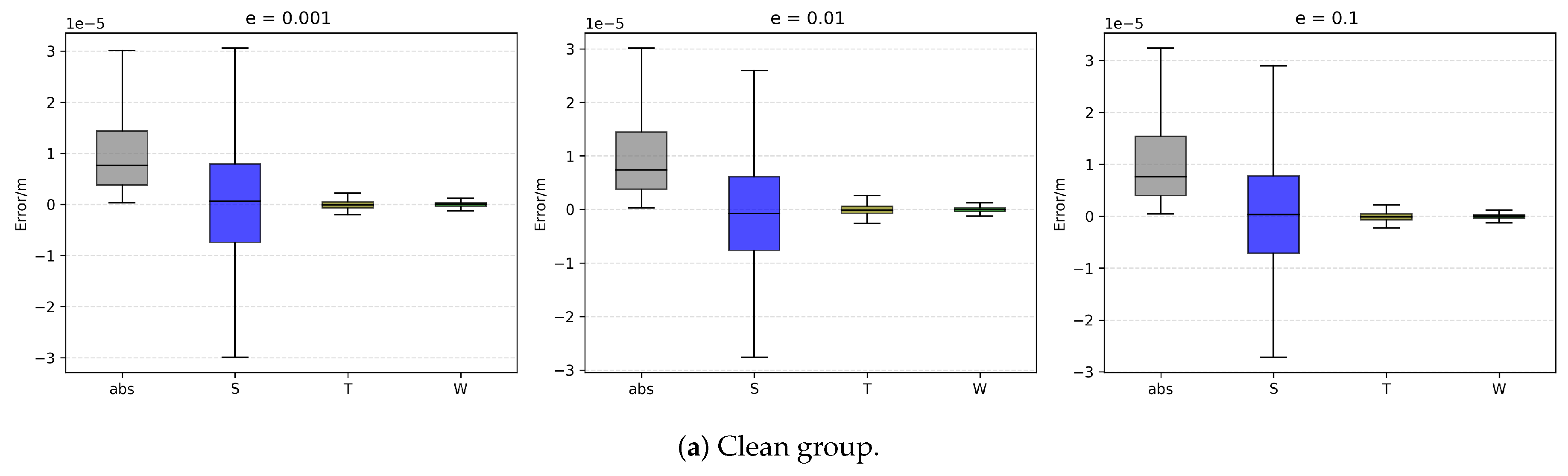
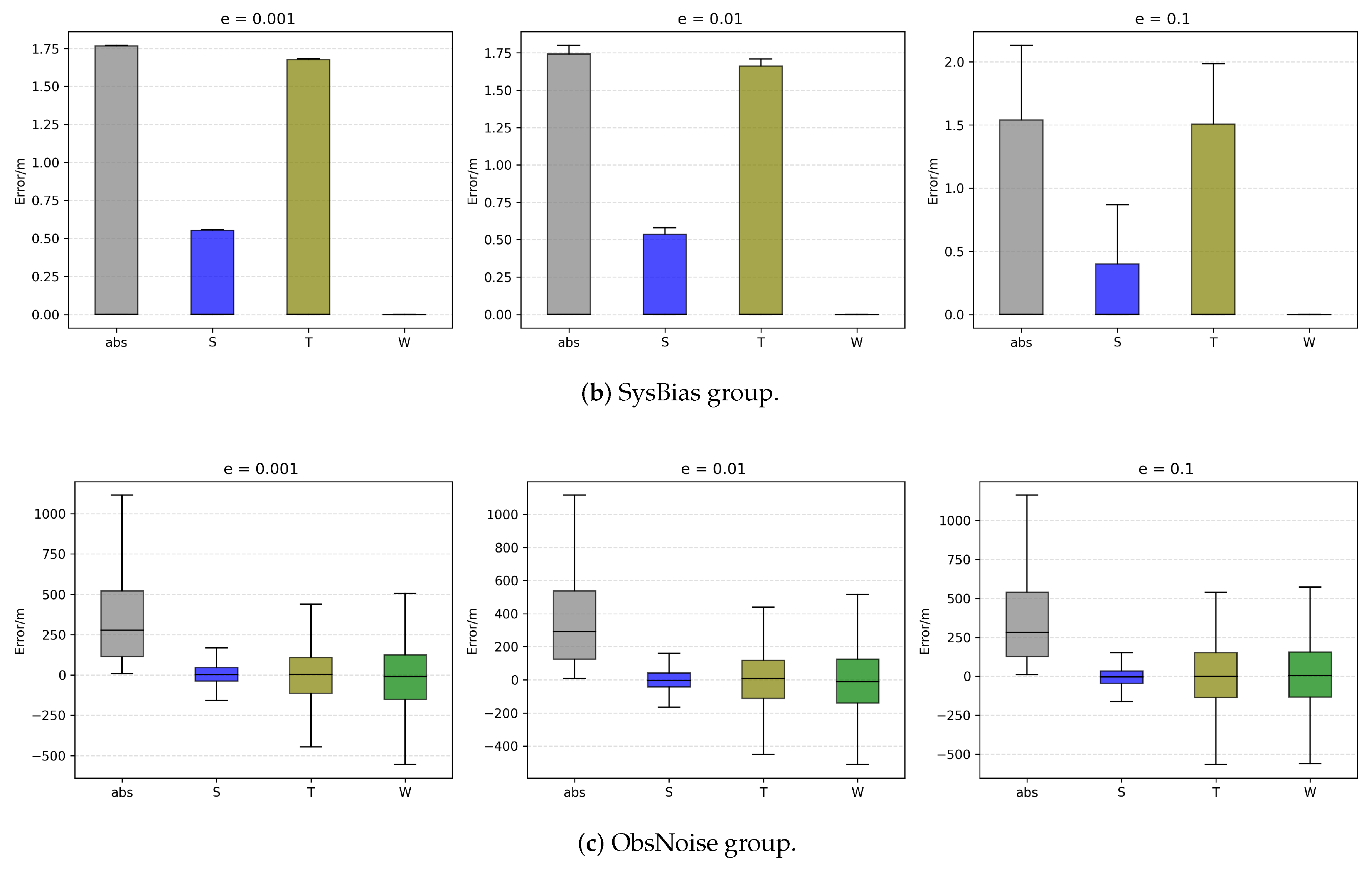
Figure 5.
Forecast error scatter plot of the Clean group.
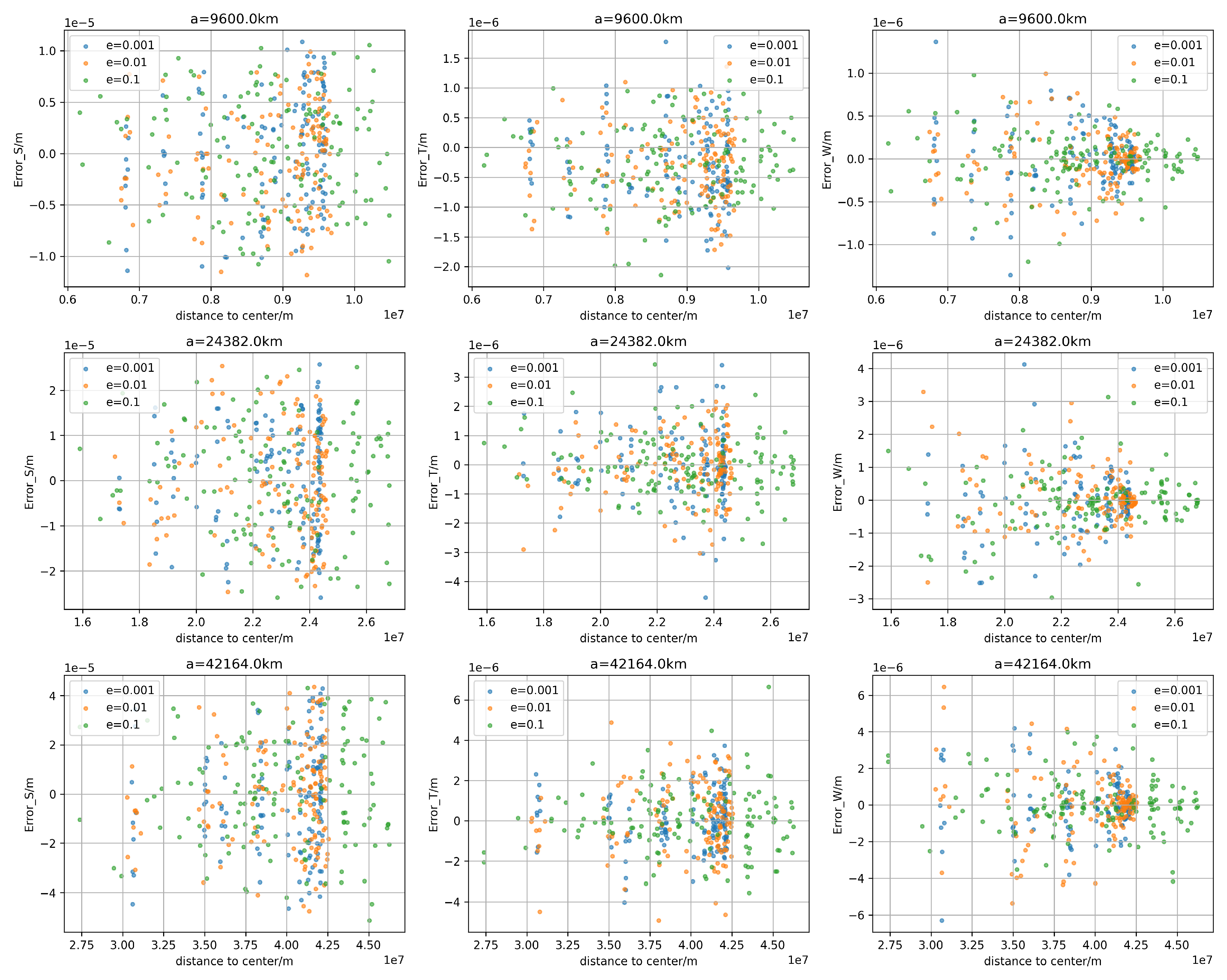
Figure 6.
Forecast error scatter plot of the SysBias group.
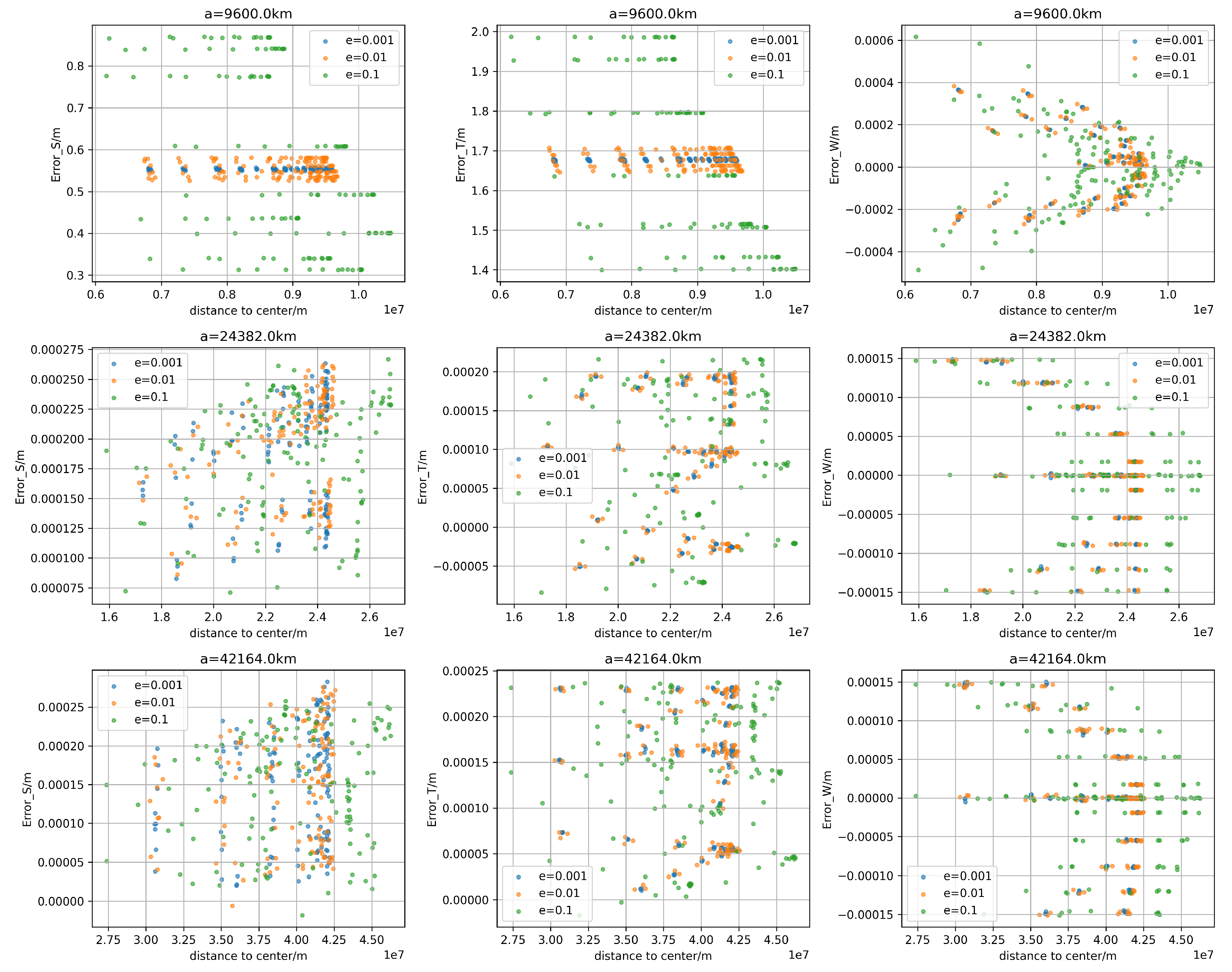
Figure 7.
Forecast error scatter plot of the ObsNoise group.
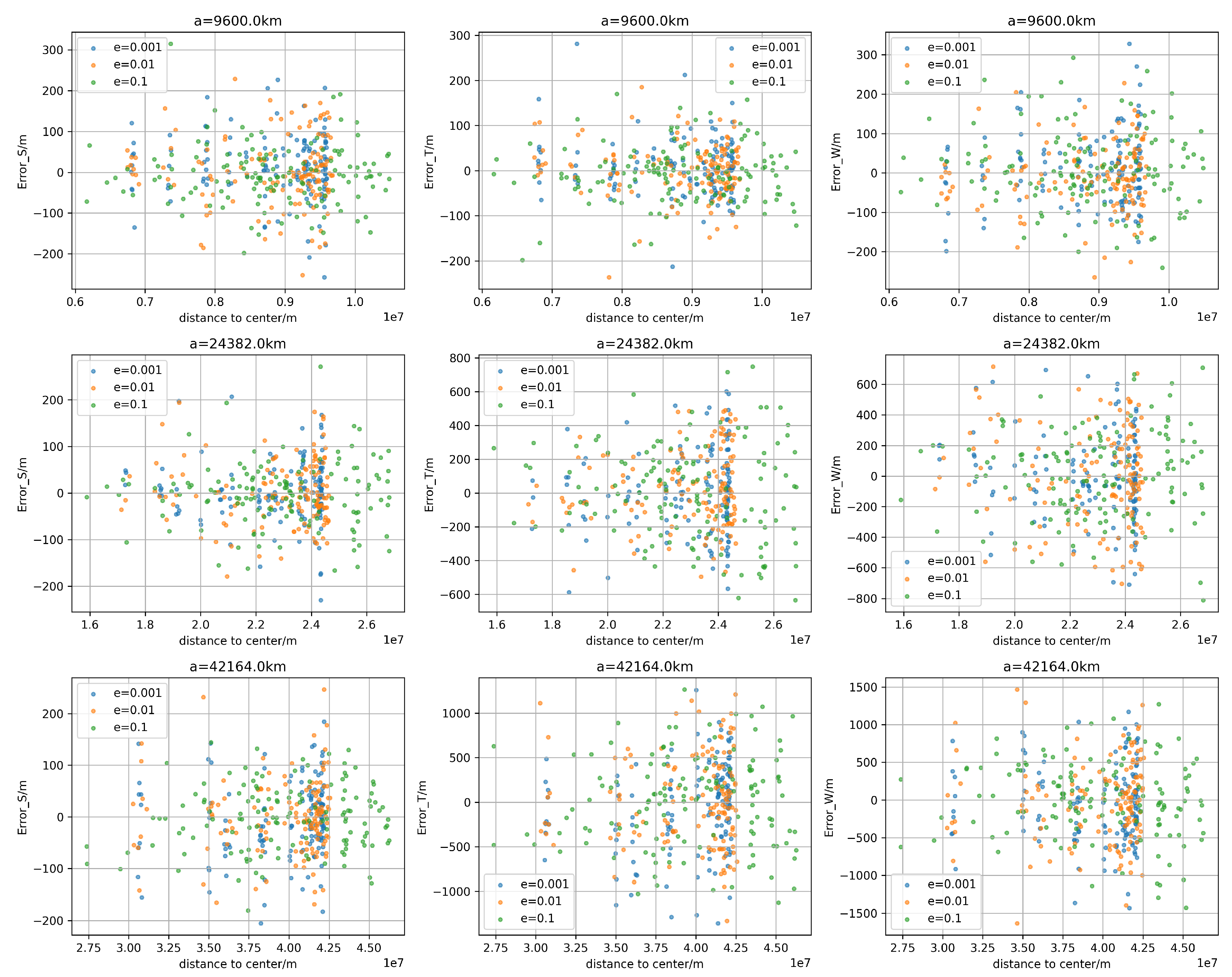

Table 1.
Orbital Parameter Values.
| Parameter | Symbol | Values | Unit |
|---|---|---|---|
| Semi-major axis | a | 9600, 24382, 42164 | km |
| Eccentricity | e | 0.001, 0.01, 0.1 | – |
| Inclination | i | 5, 15, 25, 35, 45 | ○ |
| Right ascension of node | 0, 120, 240 | ○ | |
| Argument of perigee | 0, 120, 240 | ○ |
Table 2.
Perturbation Factors
| Perturbation | Symbol | |
|---|---|---|
| Earth oblateness | ||
| Atmospheric drag | ||
| Solar radiation pressure |
Table 3.
Rank-Sum Sensitivity Test Results
| Scene | Factor | Error | H | p |
|---|---|---|---|---|
| Clean | Inclination | abs | 0.929 | 0.9203 |
| Clean | Inclination | R | 9.511 | 0.0495 |
| Clean | Inclination | T | 8.021 | 0.0908 |
| Clean | Inclination | N | 5.047 | 0.2825 |
| Clean | Semi-Major Axis | abs | 370.698 | 0.0000 |
| Clean | Semi-Major Axis | R | 0.569 | 0.7523 |
| Clean | Semi-Major Axis | T | 26.254 | 0.0000 |
| Clean | Semi-Major Axis | N | 0.543 | 0.7624 |
| Clean | Eccentricity | abs | 0.493 | 0.7814 |
| Clean | Eccentricity | R | 1.799 | 0.4067 |
| Clean | Eccentricity | T | 0.344 | 0.8418 |
| Clean | Eccentricity | N | 0.088 | 0.9568 |
| SysBias | Inclination | abs | 0.323 | 0.9883 |
| SysBias | Inclination | R | 7.676 | 0.1042 |
| SysBias | Inclination | T | 2.105 | 0.7165 |
| SysBias | Inclination | N | 0.239 | 0.9934 |
| SysBias | Semi-Major Axis | abs | 809.385 | 0.0000 |
| SysBias | Semi-Major Axis | R | 832.716 | 0.0000 |
| SysBias | Semi-Major Axis | T | 843.947 | 0.0000 |
| SysBias | Semi-Major Axis | N | 0.006 | 0.9972 |
| SysBias | Eccentricity | abs | 0.467 | 0.7916 |
| SysBias | Eccentricity | R | 0.317 | 0.1042 |
| SysBias | Eccentricity | T | 0.158 | 0.7165 |
| SysBias | Eccentricity | N | 0.101 | 0.9934 |
| ObsNoise | Inclination | abs | 2.352 | 0.6713 |
| ObsNoise | Inclination | R | 3.728 | 0.4441 |
| ObsNoise | Inclination | T | 2.426 | 0.6580 |
| ObsNoise | Inclination | N | 1.934 | 0.7478 |
| ObsNoise | Semi-Major Axis | abs | 713.261 | 0.0000 |
| ObsNoise | Semi-Major Axis | R | 1.254 | 0.5343 |
| ObsNoise | Semi-Major Axis | T | 0.227 | 0.8928 |
| ObsNoise | Semi-Major Axis | N | 1.675 | 0.4329 |
| ObsNoise | Eccentricity | abs | 0.431 | 0.8059 |
| ObsNoise | Eccentricity | R | 2.518 | 0.2840 |
| ObsNoise | Eccentricity | T | 0.048 | 0.9761 |
| ObsNoise | Eccentricity | N | 2.892 | 0.2355 |
Table 4.
The forecast error of the Chebyshev method based on 3-minite LEO ephemeris data
| time/sec | 4 | 8 | 12 | 16 | 20 |
| error for Chebyshev [8,10] /m | 14.61 | 48.11 | 113.53 | 228.20 | 419.18 |
| error for Chebyshev [10,18] /m | 2.45 | 8.32 | 21.29 | 48.87 | 99.81 |
| error for Chebyshev [14,30] /m | 4.67 | 24.41 | 80.77 | 215.76 | 510.60 |
Table 5.
The forecast error of the Dynamical Extrapolation Method based on 3-minite ephemeris data
| time/min | 0 | 1 | 2 | 3 | 4 | 5 | 6 | 7 | 8 | 9 | 10 |
| error for LEO/meter | 5.9 | 9.8 | 17.9 | 29.0 | 42.2 | 56.4 | / | / | / | / | / |
| error for GEO/meter | 56.5 | 56.6 | 56.4 | 56.2 | 56.6 | 56.3 | 56.3 | 56.5 | 56.3 | 56.3 | 56.5 |
Disclaimer/Publisher’s Note: The statements, opinions and data contained in all publications are solely those of the individual author(s) and contributor(s) and not of MDPI and/or the editor(s). MDPI and/or the editor(s) disclaim responsibility for any injury to people or property resulting from any ideas, methods, instructions or products referred to in the content. |
© 2025 by the authors. Licensee MDPI, Basel, Switzerland. This article is an open access article distributed under the terms and conditions of the Creative Commons Attribution (CC BY) license (https://creativecommons.org/licenses/by/4.0/).
Copyright: This open access article is published under a Creative Commons CC BY 4.0 license, which permit the free download, distribution, and reuse, provided that the author and preprint are cited in any reuse.


