Less for Better: A View Filter-Driven Graph Representation Fusion Network

1. Introduction

Graph-structured data increasingly exhibit multi-view characteristics with the development of graph representation learning. For instance, social networks encompass multiple views, including user profiles, interaction histories, and content preferences. Multi-view learning is crucial as it integrates diverse perspectives, enhancing model performance on downstream tasks and enabling more reliable analysis of complex data [1,2]. Multi-view learning has witnessed significant advances across diverse domains, including computer vision [3], natural language processing [4], and bioinformatics [5].

Recently, Owing to the powerful capability of Graph Neural Networks (GNNs) in capturing complex structural relationships and semantic information, the collaboration between multi-view learning and GNNs facilitates the extraction of view-specific representations and the discovery of inter-view correlations [6,7]. This collaboration enables multi-view GNNs to fully exploit complementary information distributed across views, leading to their promising performance in various real-world applications [8,9]. For example, in recommendation systems, multi-view GNNs fuse heterogeneous user–item interactions, achieving excellent recommendation accuracy.

Currently, to enhance the effectiveness of multi-view fusion in representation learning, existing approaches typically employ attention [10], gating [11], alignment [12], or fusion modules [13] to jointly integrate information from all views. These methods assign weights or scores to each view and aggregate views accordingly, allowing models to emphasize informative views while suppressing irrelevant ones. However, these approaches aggregate all views based on the assumption that all views contribute positively to the learning process. We argue that this assumption is not always valid, thereby we conduct a preliminary experiment to examine its validity. To assess the contribution of each view, we measured its information content using information entropy [14] . A greedy strategy was applied, where the raw view (Raw) was sequentially integrated with other views (V1, V2, V3) in descending order of entropy. As illustrated in Figure 1, the classification accuracy initially increases but subsequently declines as more views are added, indicating that irrelevant views may interfere with model performance. Therefore, it is vital to design an effective mechanism to identify and retain only the views that contribute positively to representation, while filtering out irrelevant views that contribute negatively.

To address the above issue, we proposes a novel multi-view representation learning framework called a View filter-driven graph representation fusion network named ViFi. We advocate a " less for better " principle, aiming to obtain superior representations by leveraging fewer yet more informative views.

Initially, entropy-based adaptive view filter is designed to identify and retain only the most informative views in a multi-view learning system, filtering out irrelevant views. The filter quantifies each view’s information content through feature–topology entropy characteristics [15], which effectively reflect the uncertainty and diversity of feature and topology distributions, serving as an indicator of a view’s information richness. By maximizing an entropy-based objective function, the module adaptively determines the optimal number of views to retain, filtering most informative views while discarding irrelevant views. The objective is formulated to reward views with substantial feature–topology entropy while penalizing irrelevance, thereby promoting a compact subset that preserves maximal informational diversity. The filter further stabilizes the subsequent fusion process by providing a compact and informative set of views.

In addition, to promote more effective fusion of informative views, we propose an optimized fusion mechanism that is introduced after filtering to adaptively determine the optimal integration strategy which yields the most informative representations. A novel information gain function is proposed to evaluate candidate view groupings based on entropy balance and structural complementarity. Entropy balance is achieved by normalizing the entropy of each view matrix and computing an equilibrium degree, which encourages uniform information contribution and avoids interference in fusion. Structural complementarity is enforced by normalizing structural differences and defining an information-gain term that favors the grouping of view matrices exhibiting significant topological diversity. By selecting the subset that maximizes overall group gain as optimal integration strategy, this module achieves balanced and complementary fusion, thereby facilitating effective collaboration among views.

To conclude, the main contributions of this study are presented as follows:

(1) A novel multi-view representation learning framework is proposed, which systemically combines view filtering with optimized fusion to produce compact, informative multi-view graph representations.

(2) An entropy-based adaptive view filter is developed, which evaluates view contribution through feature–topology entropy and dynamically filters the most informative views to reduce irrelevance and enhance complementarity.

(3) A novel information gain function is designed to evaluate the contribution of different view integration strategies and guide the selection of an optimal integration strategy that achieves entropy balance and structural complementarity, thereby strengthening inter-view collaboration.

(4) Based on comprehensive experiments on classification and clustering tasks, the proposed method consistently achieves superior performance over existing state-of-the-art approaches.

2. Related work

2.1. Multi-View Learning

Multi-view learning exploits complementary information from different data perspectives, whose integration enables more comprehensive representations. Traditional multi-view learning methods can be divided into three major categories [16] : co-training style algorithms [17,18] , co-regularization style algorithms [19] and margin-consistency style algorithms [20,21] . For instance, Qiao et al. [22] proposed Deep Co-Training, which trains multiple networks as distinct views under adversarial perturbations to maintain complementary and diverse view representations. Wang et al. [23] introduced Deep Canonically Correlated Autoencoders (DCCAE), combining CCA with autoencoder reconstruction to co-regularize representations across views. The hybrid objective offers a flexible way to align and denoise multi-view features. Mao et al. [24] proposed Soft-Margin-Consistency Multi-View MED (SMVMED), relaxing hard margin-equality constraints into a soft consistency principle to improve scalability while preserving discriminative power. However, these studies generally integrate all available views, overlooking the potential interference of irrelevant views in graph representation learning. Inspired by these works, we attempt to design a view filtering mechanism that filtering most informative views while discarding irrelevant views.

2.2. Multi-View Representation Fusion

As a critical component of multi-view learning, multi-view representation fusion is not a novel topic, and it has been extensively explored in a range of existing studies. Based on the time of multi-view fusion during the learning process, traditional works can be divided into two primary types [25]. (1) Early fusion integrates features from multiple views at the feature level before model training through typical methods such as feature concatenation, pooling-based integration and convolutional fusion. For example, Kachole et al. [26] concatenated RGB and event-stream features at the feature level to construct a unified multi-view representation, which effectively enhanced view complementarity and improved segmentation accuracy. Wei et al. [27] aggregates per-view CNN descriptors by adaptive view pooling over a learned view-graph to obtain a unified global shape descriptor. Liang et al. [28] employs 1×1 convolutions for channel-wise fusion of LiDAR and camera features before joint detection, significantly improving multi-view 3D detection accuracy. (2) Late fusion aggregates the predictions from different views after training separate models for each view through methods such as score averaging, weighted voting, and meta-classifier stacking. For instance, Simonyan et al. [29] averaged softmax scores from spatial and temporal streams to obtain a single decision, which consistently outperformed either stream alone on multi-view action recognition. Su et al. [30] used weighted voting to aggregate the prediction scores from multiple views, enabling a more robust fusion that improved the reliability of biomarker identification. Wang et al. [31] employed a meta-classifier to integrate the cross-validated outputs of view-specific CNN classifiers, enabling stacking-based fusion that better exploited heterogeneous cues and enhanced overall prediction accuracy.

Building upon the above fusion strategies, LoGo-GNN [32] can be regarded as a hybrid fusion framework that integrates both early and late fusion principles through a local-to-global architecture. In this framework, the local module performs fusion by integrating multiple view-specific representations through fixed aggregation pathways, where neighborhood information from different local views is jointly embedded to capture interrelated patterns within each view. The global module further aligns these aggregated representations across views to ensure overall consistency. However, its architecture relies on fixed local view strategy, limiting its flexibility in adapting to heterogeneous graph structures and diverse view relationships. In our study, we inspired from LoGo-GNN and extends its local-global architecture by designing an optimised fusion mechanism that dynamically selects optimal integration strategy.

3. ViFi

3.1. Notation

We consider a graph $\mathcal{G}=(\mathcal{V},\mathcal{E})$ with adjacency matrix $\mathbf{A}$ and node-feature matrix $\mathbf{X}$. The i-th graph view is denoted by $M_i$, and S denotes the selected subset of views with $k=\left|S\right|$ the number of selected high-quality views; $T_3$ is the minimum number of views required. For each view $M_i$, $H_f\left(M_i\right)$ and $H_s\left(M_i\right)$ denote its feature entropy and topology entropy, respectively; their combination yields the view information score $I\left(M_i\right)$. A subset S is evaluated by the subset score $F\left(S\right)$. To characterize complementarity between views, we use the entropy balance $B_{ij}$ and the normalized structural difference ${\Delta }_{ij}$, whose product defines the pairwise gain $G(M_i,M_j)$; aggregating pairwise gains over S gives the group gain $G\left(S\right)$. $g(·)$denotes a GNN encoder. Table 1 summarizes the notations used in this paper.

3.2. Framework Overview

The overall structure of ViFi is illustrated in Figure 2. It mainly includes two modules. (1) Entropy-based adaptive view filter evaluates each view based on feature and topological entropy characteristics to adaptively filter those with the highest informational utility, thereby establishing a compact and diverse set of informative views. (2) Optimized fusion mechanism employs a novel information gain function, which is constructed from entropy balance and normalized structural difference across views. It effectively fuses the representations by dynamically selecting optimal view integration strategy that maximize the group gain.

3.3. Entropy-Based Adaptive View Filter

Multi-view learning often contains irrelevant views. For example, in recommendation graphs, views derived from clicks, purchases, and wishlists may overlap in signal, and sparsity varies across them. In molecular property prediction, 2D topology, 3D conformers, and substructure fingerprints provide complementary but uneven information. Passing all views downstream raises computation and risks over-fitting to noisy or irrelevant signals. Therefore, entropy-based adaptive view filter is designed to address this issue by ranking and filtering only informative views and by adapting the number of retained views to the data.

We quantify the information content in each view by feature–topology entropy characteristics [15]: feature entropy and topology entropy. Feature entropy reflects uncertainty in node attributes under locality assumptions. Topology entropy captures higher-order topology using normalized structural statistics. Entropy is an appropriate metric here because it summarizes distributional uncertainty in a model-agnostic way and requires no task labels. Let a view $M_i=(A_i,X_i)$. We define:

$$H_f\left(M_i\right)=-\sum _i{p}_i^{\left(f\right)}log{p}_i^{\left(f\right)},H_s\left(M_i\right)=-\sum _i{p}_i^{\left(s\right)}log{p}_i^{\left(s\right)},$$

(1)

where $p^{\left(f\right)}$ and $p^{\left(s\right)}$ are normalized distributions induced by features and structure following Luo et al [15]. We combine them as:

$$I\left(M_i\right)=\alpha H_f\left(M_i\right)+(1-\alpha )H_s\left(M_i\right),$$

(2)

where $\alpha \in [0,1]$, and use $I\left(M_i\right)$ only to drive the filter. Higher scores indicate that the view contains richer information and greater complementarity.

We now use entropy to filter a subset of views and to adaptively decide how many to keep. The key idea is to retain views with high information content while preventing the inclusion of an excessively large set that would reintroduce redundancy and increase computational cost. We score any candidate subset S by:

$$F\left(S\right)={\displaystyle \frac{1}{\left|S\right|}}\sum _{M_i\in S}I\left(M_i\right)-\mu g\left(\right|S\left|\right),\left|S\right|\ge T_3.$$

(3)

Here S denotes the filtered set of candidate views. $I\left(M_i\right)$ is the per-view information score defined above. The parameter $\mu >0$ controls the trade-off between information and complexity. The function $g(·)$ is an increasing size penalty, with common choices $g\left(n\right)=max(n-T_3,0)$ or $g\left(n\right)=n$. The constant $T_3=3$ imposes a minimum of three views to preserve basic multi-view complementarity. Maximizing $F\left(S\right)$ yields a filter that keeps high-information views and discards redundant ones while automatically determining how many views to retain:

$$S^{★}=arg\underset{S}{max}F\left(S\right).$$

(4)

This design makes the filter adaptive, reduces computation, and stabilizes downstream fusion by avoiding noisy or overlapping inputs.

Entropy-based adaptive view filter uses feature–topology entropy characteristics to quantify view information, then maximizes F(S) to select an adaptive-size subset. The module filters out irrelevant views. It preserves complementary signal and yields a compact, informative set with less redundancy. This not only improves efficiency and robustness but also reduces the burden on the subsequent fusion stage.

Algorithm 1: Entropy-based adaptive view filter
Input: Graph views $\{M_1,M_2,\dots ,M_n\}$, where each $M_i=(A_i,X_i)$; trade-off parameter $\alpha \in [0,1]$;   penalty coefficient $\mu >0$; minimum view count $T_3$; size penalty function $g(·)$.
Output: Filtered subset of views $S^{*}$.
1:	for each view $M_i$ do
2:	Compute feature entropy $H_f\left(M_i\right)$ and topology entropy $H_s\left(M_i\right)$ via Eq.1;
3:	Calculate feature–topology entropy as view content information via Eq.2;
4:	end for
5:	Initialize: candidate subset S with $\left|S\right|\ge T_3$;
6:	Compute the subset score $F\left(S\right)$ by combining the average information score of views in S with   a penalty term based on the subset size, as defined in Eq.3;
7:	Select the most informative subset $S^{*}$ by maximizing the subset score $F\left(S\right)$ over all candidate   subsets, following the process in Eq.4;
8:	return $S^{*}$.

3.4. Optimized Fusion Mechanism

Furthermore, to enable more effective fusion of informative views, we introduce a fusion mechanism based on a local-to-global framework, which promotes hierarchical integration of view-specific information and enhances overall representation consistency. To further investigate how different integration strategies influence representation quality, we conduct a preliminary experiment that evaluates the effect of different integration strategies on node classification accuracy across multiple datasets. The results shown in Figure 3 , indicate that varying integration strategies lead to significant differences in classification performance. This observation motivates the need to adaptively identify the most effective view integration strategy for fusion mechanism.

After obtaining a set of informative views, we need to decide which subset of the filtered views should be integrated so that their fused representation is maximally informative. The fusion objective is to balance the information contribution of each view and to exploit structural complementarity among them. To achieve this, we introduce a novel information gain function that scores candidate groups and selects the subset with the highest gain.

The goal of this module is to select an optimal subset S of filtered view matrices for joint fusion. Let $\{M_1,\dots ,M_n\}$ represent the candidate view matrices obtained from Module 1. We group these matrices into sets of size $k\ge 2$, since fusion requires at least two views. The objective is to find the grouping that maximizes the overall fusion score. Each group should maintain balanced information entropy across views and preserve structural complementarity. In this way, the fusion process avoids dominance by a single view and reduces irrelevance among similar structures.

To quantify these ideas, we start by defining a pairwise gain $G(M_i,M_j)$ between any two view matrices $M_i$ and $M_j$. First, let $H\left(M_i\right)$ denote the Shannon entropy of matrix $M_i$, interpreted as the amount of information it contains. We define two factors:

1) Entropy balance:

$$B_{ij}={\displaystyle \frac{min\left(H\left(M_i\right),H\left(M_j\right)\right)}{max\left(H\left(M_i\right),H\left(M_j\right)\right)}},$$

(5)

where lies in $[0,1]$. When $H\left(M_i\right)\approx H\left(M_j\right)$, $B_{ij}$ is close to 1, indicating balanced information; if one entropy is much smaller than the other, $B_{ij}$ approaches 0, reflecting imbalance.

2) Normalized structural difference:

$${\Delta }_{ij}={\displaystyle \frac{{\parallel M_i-M_j\parallel }_F}{{\parallel M_i\parallel }_F+{\parallel M_j\parallel }_F}},$$

(6)

where ${\parallel ·\parallel }_F$ is the Frobenius norm. This measures how different the two matrices are, normalized by their magnitudes. The value ${\Delta }_{ij}\in [0,1]$ is 0 if $M_i=M_j$ (no structural difference) and approaches 1 as the difference grows large relative to their norms. This normalization makes ${\Delta }_{ij}$ comparable across different data scales.

The pairwise gain is then defined as the product of these two factors:

$$G(M_i,M_j)=B_{ij}\times {\Delta }_{ij}={\displaystyle \frac{min\left(H\left(M_i\right),H\left(M_j\right)\right)}{max\left(H\left(M_i\right),H\left(M_j\right)\right)}}·{\displaystyle \frac{{\parallel M_i-M_j\parallel }_F}{{\parallel M_i\parallel }_F+{\parallel M_j\parallel }_F}}.$$

(7)

By construction, $G(M_i,M_j)$ is high only when $M_i$ and $M_j$ have comparable entropies ( $B_{ij}$ is near 1) and significant structural difference ( ${\Delta }_{ij}$ is large). If either condition fails (one view dominates in entropy or the two views are nearly identical), the product ensures $G(M_i,M_j)$ is small. This multiplicative form naturally enforces a " both-or-none " threshold: both entropy balance and structural complementarity must be present for a large gain. It is worthy to note that no additional parameters are needed in this metric.

Next, we extend the pairwise gain to an entire group (subset) of views. For any subset $S\subseteq \{M_1,\dots ,M_n\}$ of size $\left|S\right|=k$, we define its group gain $G\left(S\right)$ as the average of all pairwise gains within the group:

$$G\left(S\right)={\displaystyle \frac{1}{\left(\genfrac{}{}{0pt}{}{k}{2}\right)}}\sum _{\begin{array}{c}{M}_i,M_j\in S\\ i<j\end{array}}G(M_i,M_j).$$

(8)

This average pairwise gain is the group quality score. The mean over $\left({\displaystyle \genfrac{}{}{0pt}{}{k}{2}}\right)$ pairs normalizes for group size. High $G\left(S\right)$ indicates complementary structure and balanced information. A weak member lowers many pair scores and reduces the average. Hence $G\left(S\right)$ is a reliable indicator of fusion value. By maximizing the overall group gain $G\left(S\right)$ to adaptively identify the view subset corresponding to the optimal integration strategy, this module achieves a balanced and complementary fusion, thereby facilitating effective collaboration among views.

Algorithm 2: Optimized fusion mechanism
Input: Filtered view set $\{M_1,M_2,\dots ,M_m\}$; GNN encoder $g(·)$; group size constraint $k\ge 2$;
Output: Fused representation $\tilde{Y}$.
1:	for each pair of views $(M_i,M_j)$ do
2:	Compute entropy balance $B_{ij}$ and normalized structural difference ${\Delta }_{ij}$ via Eq.5, 6;
3:	Determine the pairwise gain $G(M_i,M_j)$ by multiplying the entropy balance and structural difference metrics to assess complementarity via Eq.7;
4:	end for
5:	for each candidate subset $S\subseteq \{M_1,\dots ,M_m\}$ with $\left|S\right|=k$ do
6:	Compute the group gain by averaging all pairwise gains within the subset to evaluate overall fusion potential via Eq.8 ;
7:	end for;
8:	Select the subset as optimal view integration strategy by identifying the candidate with the highest group gain value;
9:	Fuse the subset using $g(·)$ and attention mechanism to integrate their representations;
10:	Return $\tilde{Y}$.

3.5. Model Details

Our framework is compatible with a wide range of graph neural network models, imposing no architectural limitations. In this study, to keep the design concise, we adopt a standard one-layer Graph Convolutional Network [33] as the basic module used to merge the representations.

$$g(·):{\mathbb{R}}^{N\times F}\times {\mathbb{R}}^{N\times N}\to {\mathbb{R}}^{N\times F_h}.$$

(9)

Its propagation rule is:

$$g(\mathbf{X},\mathbf{A})=\sigma \left(\tilde{\mathbf{A}}\mathbf{X}\Theta \right),$$

(10)

where $\sigma (·)$ is a standard nonlinearity (e.g., ReLU, softmax, sigmoid, or tanh). The symmetrically normalized adjacency is:

$$\tilde{\mathbf{A}}={\widehat{\mathbf{D}}}^{-{\displaystyle \frac{1}{2}}}\widehat{\mathbf{A}}{\widehat{\mathbf{D}}}^{-{\displaystyle \frac{1}{2}}},\widehat{\mathbf{A}}=\mathbf{A}+\mathbf{I},\widehat{\mathbf{D}}=\mathbf{D}+\mathbf{I}.$$

(11)

$\mathbf{X}\in {\mathbb{R}}^{N\times F}$ contains node features and $\mathbf{A}\in {\mathbb{R}}^{N\times N}$ encodes graph connectivity; adding $\mathbf{I}$ introduces self-loops. The matrix $\Theta \in {\mathbb{R}}^{F\times F_h}$ maps F-dimensional inputs to $F_h$-dimensional fused features. Symmetric normalization scales messages by node degrees for stable training. This single layer mixes information over one hop, and any other GNN backbone can replace it without altering the fusion pipeline.

Local and global view encoders. Each view encoder is composed of a GCN-based encoder together with its corresponding set of input views. These inputs may consist of different combinations of views, selected according to the chosen integration strategy. Rather than operating on a single view as in a typical GCN, both the local and global encoders receive multiple views simultaneously and generate their representations by applying mean pooling to the aggregated features:

$$g_{{\Theta }_{\theta }}={\displaystyle \frac{1}{k}}\sum _{{\mathcal{G}}_j\in \{{\mathcal{G}}_1,{\mathcal{G}}_2,\dots ,{\mathcal{G}}_k\}}ReLU\left(\tilde{\mathit{A}}{\mathit{X}}_j{\Theta }_{\theta }\right).$$

(12)

Attention mechanism. To merge embeddings from the local and global encoders, we use an attention module to obtain a richer semantic representation.

Given m embeddings ${\mathit{H}}_1,{\mathit{H}}_2,\dots ,{\mathit{H}}_m$, attention scores their contributions:

$$({\alpha }_1,{\alpha }_2,\dots ,{\alpha }_m)=att({\mathit{H}}_1,{\mathit{H}}_2,\dots ,{\mathit{H}}_m).$$

(13)

Here ${\alpha }_i\in {\mathbb{R}}^{N\times 1}$ gives node-wise weights for ${\mathit{H}}_i$. The coefficients follow ${\alpha }_{ij}=softmax\left(w_{ij}\right)$, with $w_{ij}={\mathbf{q}}_i^T·tanh({\Theta }_{att}·{\left({\mathbf{h}}_j\right)}^T+{\mathbf{b}}_i)$, where ${\mathbf{q}}_i\in {\mathbb{R}}^{F^{\prime }\times 1}$ is a shared attention vector, ${\Theta }_{att}\in {\mathbb{R}}^{F^h\times F^{\prime }}$ is the weight matrix, and ${\mathbf{b}}_i\in {\mathbb{R}}^{F^{\prime }\times 1}$ is the bias.

The fused embedding is the attention-weighted sum:

$$\mathit{H}={\alpha }_1·{\mathit{H}}_1+{\alpha }_2·{\mathit{H}}_2+...+{\alpha }_m·{\mathit{H}}_m.$$

(14)

3.5.1. Semi-Supervised Learning Architecture

In settings where only partial labels are available, typified by node classification, the framework concludes its representation extraction stage with a single-layer GCN that functions as the terminal encoder.The fused embedding $\mathbf{H}$ is subsequently processed by a single-layer Graph Convolutional Network, which functions as the final stage of encoding and generates the model’s representations $\tilde{\mathbf{Y}}$:

$$\tilde{\mathbf{Y}}=softmax\left(\tilde{\mathit{A}}\mathit{H}{\Theta }_{final}\right).$$

(15)

3.5.2. Unsupervised Learning Architecture

In unsupervised settings, incorporating a decoder enables the model to exploit self-supervised signals from the input graphs [34]. ViFi comprises a suite of encoders that capture complementary perspectives, whose outputs are aggregated into a unified embedding. Reconstruction is then achieved by pairing this fused representation with a set of decoders, each tasked with reconstituting a specific input view. Beyond the direct correspondence between input and output, an auxiliary decoder is incorporated to reconstruct the structural information of the original view. This reconstruction module is built from multiple two-layer components, with each layer crafted to serve as an approximate inverse of the encoder it mirrors.

The decoding stage produces two reconstructions: the node-feature matrix ${\tilde{\mathbf{X}}}_i$ and the recovered view topology ${\tilde{\mathbf{A}}}_{re}$. For the decoder associated with the i-th input view, the reconstructed node attributes are computed as:

$${\tilde{\mathbf{X}}}_i^{re}=softmax\left(\tilde{\mathbf{A}}ReLU\left(\tilde{\mathbf{A}}\mathbf{H}{\Theta }^{\left(0\right)}{\theta }_i^{\prime }\right){\Theta }^{\left(1\right)}{\theta }_i^{\prime }\right),$$

(16)

where ${\Theta }^{\left(l\right)}{\theta }_i^{\prime }$ represents the learnable weights associated with the i-th view-specific reconstruction decoder at layer l.

The output of decoder is:

$$\tilde{\mathbf{H}}=\tilde{\mathbf{A}}ReLU\left(\tilde{\mathbf{A}}\mathbf{H}{\Theta }_{{\theta }^{\prime }}^{\left(0\right)}\right){\Theta }_{{\theta }^{\prime }}^{\left(1\right)},{\tilde{\mathbf{A}}}^{re}=sigmoid\left(\tilde{\mathbf{H}}{\tilde{\mathbf{H}}}^T\right).$$

(17)

3.6. Training

The training objective of ViFi integrates two core terms: a complementary-learning objective and object loss [32]. The former, denoted as (${\mathcal{L}}_c$) , aims to merge information drawn from multiple encoder viewpoints, whereas the latter, (${\mathcal{L}}_o$) , drives the model to perform well on the specific downstream application.

We introducea global loss function denoted as $\mathcal{L}$ to governs the entire training process:

$$\mathcal{L}=\eta ·{\mathcal{L}}_c+(1-\eta )·{\mathcal{L}}_o.$$

(18)

Discriminator and complementary loss. To mitigate the issue that the global encoder alone may struggle to learn an optimal representation, a local encoder is incorporated to provide additional corrective signals. This design encourages the two encoding pathways to capture mutually informative cues, and the interaction between them is strengthened through a graph-based contrastive learning scheme. On this basis, the complementary objective (${\mathcal{L}}_c$) [32] is defined as follows:

$${\mathcal{L}}_c=exp(-{\displaystyle \frac{1}{\left|\mathcal{V}\right|}}\sum _{l\in \mathbf{V}}{\sum }_{i=1}^{m-1}{\sum }_{j\ne i}^m{∥{\mathbf{Z}}_{l,i}-{\mathbf{Z}}_{l,j}∥}_2).$$

(19)

where $\left|\mathcal{V}\right|$ denotes the total number of nodes, and ${\mathbf{Z}}_{l,i}$ ($1<i\le m$) represents the feature embedding of node l produced by the i-th view encoder.

Object loss for semi-supervised and unsupervised learning. For the semi-supervised setting, node classification is optimized by applying a cross-entropy objective to the embeddings corresponding to the labeled nodes:

$${\mathcal{L}}_o=-\sum _{v_k\in {\mathcal{V}}_L}\sum _j^C{\mathbf{Y}}_{kj}^{L}log\left({\tilde{\mathbf{Y}}}_{kj}\right).$$

(20)

In the unsupervised setting, the model relies on a combination of reconstruction loss and contrastive loss to realize self-supervised training. Accordingly, the task-specific loss for this scenario is formulated as follows:

$$\begin{array}{c}\hfill {\mathcal{L}}_o=\sum _{j\in \{{\mathcal{G}}_1,{\mathcal{G}}_2,\dots ,{\mathcal{G}}_k\}}{∥{\tilde{\mathit{X}}}_j-{\tilde{\mathit{X}}}_j^{re}∥}_2\\ \hfill +{\lambda }_1{∥\tilde{\mathit{A}}-{\tilde{\mathit{A}}}^{re}∥}_2+{\lambda }_2\sum _i^m\sum _{j\in \mathcal{G}se{t}_i}\sum _{k\in \mathcal{G}se{t}_i,j\ne k}{\mathcal{I}}_{j,k}^i.\end{array}$$

(21)

where ${\lambda }_1$ and ${\lambda }_2$ are hyperparameters. $\mathcal{G}se{t}_i$ is the input set for the i-th view encoder.

4. Experiments

In this section, we conduct extensive experiments to validate the superiority of ViFi and answer the following research questions.

Q1: What is the performance of ViFi in node classification and graph classification tasks?

Q2: How can we verify the advantage of the ViFi framework?

Q3: What roles are fulfilled by the individual components within the proposed framework?

Q4: In what ways is the robustness of ViFi demonstrated?

Q5: How effective is the approach when it is utilized for node-clustering applications?

Q6: To what extent do changes in hyperparameter settings influence the behavior of ViFi?

Datasets. We conduct our evaluation on six benchmark datasets, whose main statistics are listed in Table 2. Cora, Citeseer, Pubmed, and DBLP are citation networks, whereas ACM and Chameleon come from academic and Wikipedia sources respectively.

ViFi. In the experimental analysis, OURS denotes the semi-supervised variant of ViFi, whereas OURS-UN refers to its unsupervised counterpart. For the unsupervised setting, the learned representations are subsequently fed into linear classifiers, allowing the model to produce node-classification results.

Baselines. We compare ViFi with state-of-the-art methods. 1) Base encoder: GCN [33]. 2) Attention-based encoder: GAT [35], MAGCN [36], DGCN [37] and PA-GCN [38]. 3) Multi-view information fusion-based encoder for node classification: MixHop [39], N-GCN [40], MOGCN [41], MAGCN [36], DGCN [37], PA-GCN [38], LoGo-GNN[32], StrucGCN[42] and ND-GCN[43]. 4) Multi-view information fusion-based encoder for graph classification: Co-GCN [44], LGCN-FF [45], SLFNet [46], HGCN-MVSC [47], MGCN-DNS [48]. 5) Contrastive learning-based encoder: NCLA [49], PA-GCN [38], GraphCL [50], IGCL [51], and GCA [52]. 5) Unsupervised learning model: K-means, Deepwalk [53], GAE [34], and VGAE [34].

Parameter Setting. A complete list of hyperparameter settings for each dataset is provided in Table 3.

Implementation Details. Our training procedure adopts a full-batch strategy for each epoch. The method is implemented in Pytorch, and parameter updates are carried out using the Adam [54] algorithm. For the standard graph benchmarks, we randomly sample different numbers of labeled nodes per class for training, while keeping 1,000 nodes fixed for testing. In superpixel datasets, evaluation is conducted on a set of 10,000 images. All classification accuracies (ACC) are averaged over 10 independent runs using the data splits described above. The hyperparameter $\eta$ is explored across {0.05, 0.1, 0.15, …, 0.95}, while ${\lambda }_1$ and ${\lambda }_2$ are adjusted within {0, 0.1, 0.2, …, 1}. Additionally, the cosine-threshold is tuned in {0.1, 0.15, 0.2, …, 0.5}, and k is varied over {5, 10, 15, …, 30}. The final results for each dataset are reported using the hyperparameter combination and iteration count that yield optimal performance.

Evaluation Metrics. Following established practices in node and graph classification, we evaluate the performance of both baseline methods and ViFi on node classification tasks using classification accuracy (ACC). For each dataset, ACC is computed across all test samples. In addition, to assess clustering effectiveness, we employ normalized mutual information (NMI) [55] and adjusted rand index (ARI) [56], providing complementary measures of how well ViFi and competing approaches capture underlying cluster structures.

Table 4. Notation description.

Notation	Description
Raw	The raw input view.
RawC	The convolution augmentation view via Equation (22).
PR	The augmented view based on raw view relations.
PC	The augmented view based on cosine similarity view relations.
PK	The augmented view based on kNN view relations.
Global	Learned representation of global views ({RAW, PC, PK}).
Local1	Learned representation of local views ({RAW, PC}).
Local2	Learned representation of local views ({RAW, PK}).
Local3	Learned representation of local views ({PC, PK}).
Local-Global	Fused representation from the local-to-global views.
No-Opt (manual)	Fusion without optimization; a fixed manual strategy is used to integrate filtered views.
Random-Select (avg)	Randomly selects view subsets of the same size for fusion and averages the results.
Only-Entropy	Employs only the entropy-balance term in the gain function.
Only-Structure	Employs only the normalized structural-difference term in the gain function.
Greedy-by-Entropy	Sequentially adds views based on their individual information scores until the gain ceases to improve.
Full (Ours)	Complete optimized fusion mechanism using both entropy balance and structural complementarity to adaptively select the optimal view integration.

Table 4. Notation description.

Notation	Description
Raw	The raw input view.
RawC	The convolution augmentation view via Equation (22).
PR	The augmented view based on raw view relations.
PC	The augmented view based on cosine similarity view relations.
PK	The augmented view based on kNN view relations.
Global	Learned representation of global views ({RAW, PC, PK}).
Local1	Learned representation of local views ({RAW, PC}).
Local2	Learned representation of local views ({RAW, PK}).
Local3	Learned representation of local views ({PC, PK}).
Local-Global	Fused representation from the local-to-global views.
No-Opt (manual)	Fusion without optimization; a fixed manual strategy is used to integrate filtered views.
Random-Select (avg)	Randomly selects view subsets of the same size for fusion and averages the results.
Only-Entropy	Employs only the entropy-balance term in the gain function.
Only-Structure	Employs only the normalized structural-difference term in the gain function.
Greedy-by-Entropy	Sequentially adds views based on their individual information scores until the gain ceases to improve.
Full (Ours)	Complete optimized fusion mechanism using both entropy balance and structural complementarity to adaptively select the optimal view integration.

4.1. Performance on Node and Graph Classification(Q1)

4.1.1. Performance on Node Classification

This section reports the average classification accuracy (ACC) along with its standard deviation across 10 independent trials. For reference, the results of DeepWalk [53], NCLA [49], LGCN-FF [45], and SLFNet [46] are adopted from their respective original studies. The outcomes of semi-supervised node classification are compiled in Table 5, with the key insights summarized as follows:

• Compared with the baseline models, ViFi demonstrates consistently superior performance across most datasets. Notably, the semi-supervised version of ViFi (OURS) achieves better results than its unsupervised counterpart (OURS-UN). This improvement can be explained by the fact that the semi-supervised framework of ViFi adopts an end-to-end fusion mechanism, in which the available label information effectively guides and refines the embedding fusion process during model training.
• The semi-supervised version of ViFi (OURS) consistently outperforms other models that incorporate multi-topology or multi-view information fusion, such as MAGCN, MOGCN, and PA-GCN. Moreover, the unsupervised version of ViFi (OURS-UN) also achieves better performance than most graph contrastive learning methods, including GCA and IGCL. This advantage primarily stems from ViFi’s ability to identify and retain only the views that contribute positively to representation, while filtering out irrelevant views that contribute negatively, thereby enhancing representation quality and improving the model’s robustness against noisy or irrelevant information.
• Building on the failure cases listed in Table 5, we select the Pubmed dataset as a representative example for a more detailed analysis. In this dataset, the performance of ViFi is inferior to that of the NCLA model. This phenomenon can be attributed to a key characteristic of NCLA: it employs an augmentation-based learning strategy, which facilitates effective extraction of self-supervised signals between the original graph and its augmented versions, provided that the underlying relationships in the raw graph are trustworthy. A comparable pattern emerges when examining the Citeseer dataset. In this case, ViFi also trails behind the LA-GCN model. This performance gap can be attributed to the design of LA-GCN, which incorporates a trainable local augmentation mechanism grounded in the structural relations of the original graph. Meanwhile, it places greater emphasis on enhancing the informative value of data from the perspective of feature engineering, which further explains its performance advantage over ViFi in this dataset. However, overall, ViFi continues to exhibit better performance compared with these competing approaches. The superior performance of ViFi can be mainly attributed to its entropy-driven adaptive view filter and optimized fusion mechanism. The adaptive view filter evaluates the similarity and connectivity among nodes to characterize the concentration of information distribution. Based on this, it filters the views that contain richer and more informative content for subsequent fusion. In the optimized fusion mechanism, a novel information gain function is proposed to evaluate candidate view groupings based on entropy balance and structural complementarity. It is further employed to determine the most effective integration strategy, thereby enabling a more efficient and complementary fusion of multi-view representations. The superiority of ViFi becomes particularly pronounced in the presence of noise. The following experimental section examines and quantifies the robustness of the model.

4.1.2. Performance on Graph Classification

We use the multi view datasets for graph classification and take GCN-fusion [33], Co-GCN [44], LGCN-FF [45], SLFNet [46], HGCN-MVSC [47] and MGCN-DNS [48] as baselines. The reported classification accuracy (ACC) represents the average over 10 independent runs. Graph classification outcomes are summarized in Table 6, demonstrating that ViFi maintains strong competitiveness in graph-level classification tasks.

4.2. ViFi Architecture Study (Q2)

To simplify the analysis, we employ only the best-performing variant of ViFi (OURS) built upon a semi-supervised learning framework. The model is applied to node classification and semantic similarity tasks on the Cora dataset, providing additional validation for the effectiveness of the proposed entropy-based adaptive view filtering and the optimized fusion strategy.

• Multi views-GCN+MLP: A GCN framework combining local and global encoder views via MLP is utilized to perform node classification tasks;
• Multi views-GAT+GAT: A graph attention network (GAT) architecture that merges local and global encoder views using a single-layer GAT is employed for node level classification tasks;
• Global-GCN+GCN: A GCN architecture adopting a global encoder perspective, implemented with a single-layer GCN for node classification tasks;
• OURS-UN-w/o: ViFi implemented under an unsupervised learning framework, operating without the complementary loss term ${\mathcal{L}}_c$;
• OURS-w/o: ViFi implemented under an semi-supervised learning framework, operating without the complementary loss term ${\mathcal{L}}_c$;
• OURS-UN: ViFi configured within an unsupervised learning framework;
• OURS: ViFi configured within an semi-supervised learning framework;

These results lead to several noteworthy observations, as discussed below:

• To further assess the efficacy of the ViFi framework, we utilize a standard MLP or a Graph Attention Network as the terminal classifier. The experimental results indicate that incorporating graph attention networks (GAT) yields superior performance compared with both the MLP-based and our proposed configurations. This improvement suggests that GAT provides a more efficient mechanism for capturing the topological dependencies within the fused node representations. Moreover, the performance of our model surpasses that of the Multi-view GCN+MLP, implying that the fusion process preserves the essential relational patterns among nodes.
• Compared with the Global-GCN+GCN variant, ViFi delivers superior results, underscoring the necessity of incorporating localized structural cues when global information is sparse or partially missing, as is often the case under limited label supervision. Furthermore, architectures that jointly exploit global and local views tend to exhibit more stable and effective behavior than approaches relying solely on a global-view encoder.
• Acquiring complementary information from different views plays a vital role. As shown in Table 7, the ViFi ($\mathbf{OURS}-\mathbf{UN}$ and $\mathbf{OURS}$) trained with the global loss function achieves better performance than the ViFi trained solely with the object loss ${\mathcal{L}}_o$. This observation further validates our rationale for introducing the global loss function.

4.3. Ablation Study (Q3)

The effectiveness of the proposed ViFi is confirmed through the comparative experiments discussed above. In addition, to further validate the contribution of each individual component within ViFi, we conduct a series of ablation studies in this subsection.

4.3.1. Entropy-Based Adaptive View Filter

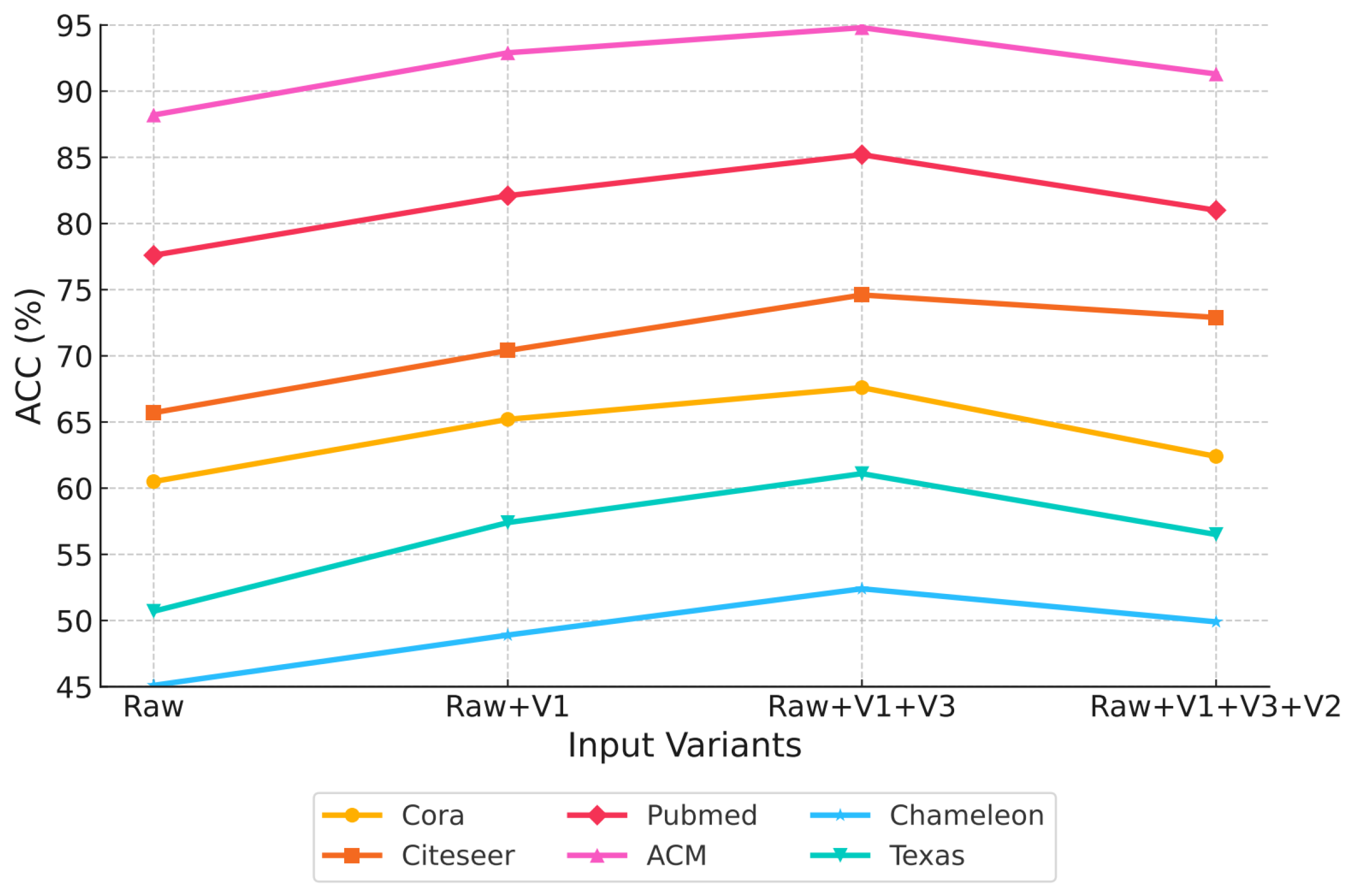
First, we apply various aggregation strategies to generate augmented graphs, each serving as a distinct view. For comparison, we incorporate the GCN aggregation method [33] into the graph augmentation process (Equation 22). Table 4 summarizes the descriptions of the various views. To visualize the representational capacity of each view (PR, PC, RawC, Raw), a broken-line chart is employed, tracking changes after each iteration. The alignment between each augmented view and the original input view (Raw) is subsequently quantified by examining their semantic similarity. Both the augmented and original views are encoded using a shared GCN encoder under identical parameter settings, and their learned graph representations are subsequently compared to assess semantic alignment.

The results in Table 8 indicate that the performance of augmented views varies notably across datasets, reflecting the distinct structural and semantic characteristics captured by each view. The PC view attains the highest accuracy on the Cora and ACM datasets, suggesting that cosine similarity preserves meaningful feature correlations beneficial for classification, while the PK view performs slightly better on Pubmed, implying that neighborhood-based relations are more informative in this dataset. Such inconsistency among single views highlights the necessity of filtering and integrating multiple complementary views. When multiple views are combined, classification accuracy improves substantially compared with individual views. Among them, Raw+PC+PK consistently achieves the best results across all datasets, indicating that combining feature-similarity and structural-proximity views enhances the representational capacity of the model and leads to more effective multi-view learning.

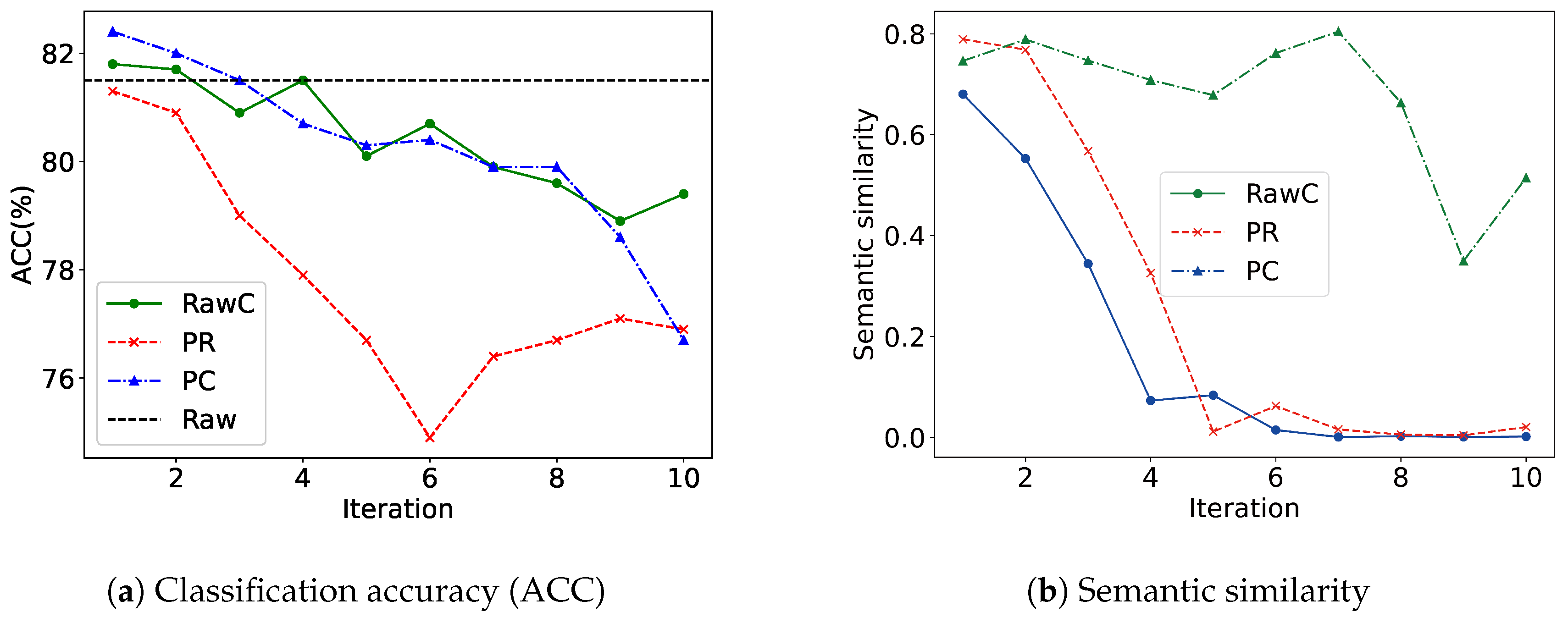
The analysis of semantic similarity and representation ability of Figure 4 provides a key explanation for this phenomenon. The figure shows that the semantic similarity and representation ability between different views show different evolution trajectories with the change of the number of iterations. The PC view can obtain higher representation ability with fewer iterations, and maintain a moderate semantic distance from the original view, which can provide effective complementary information, but said the ability to improve the limited. This inconsistency in performance and properties implies that directly fusing all views without any filtering mechanism may introduce interfering or task-irrelevant views, thereby degrading model performance. Moreover, the model would fail to adaptively identify the most informative views for the given task, ultimately resulting in suboptimal fusion outcomes. Therefore, a filtering mechanism that evaluates and adaptively filters views is essential to ensure that the fusion process focuses on the most informative and complementary views.

$${\tilde{\mathbf{x}}}_i={\widehat{\mathbf{A}}}_{i,i}{\mathbf{x}}_i+\sum _{{\mathbf{x}}_j\in \mathcal{N}\left({\mathbf{x}}_i\right)}{\widehat{\mathbf{A}}}_{i,j}{\mathbf{x}}_j.$$

(22)

4.3.2. Optimized Fusion Mechanism

Furthermore, we design a series of comparative experiments, to investigate the role of the optimized fusion mechanism. Specifically, we implement several fusion variants, including manual fusion, random subset selection, and simplified versions that retain only the entropy-balance or structural-difference term. Each variant employs the same set of filtered views obtained from the first module, ensuring that the observed differences arise solely from the fusion mechanism. The descriptions of these variants are summarized in Table 4. Subsequently, we compare their classification accuracy across multiple datasets to evaluate the impact of different fusion mechanisms.

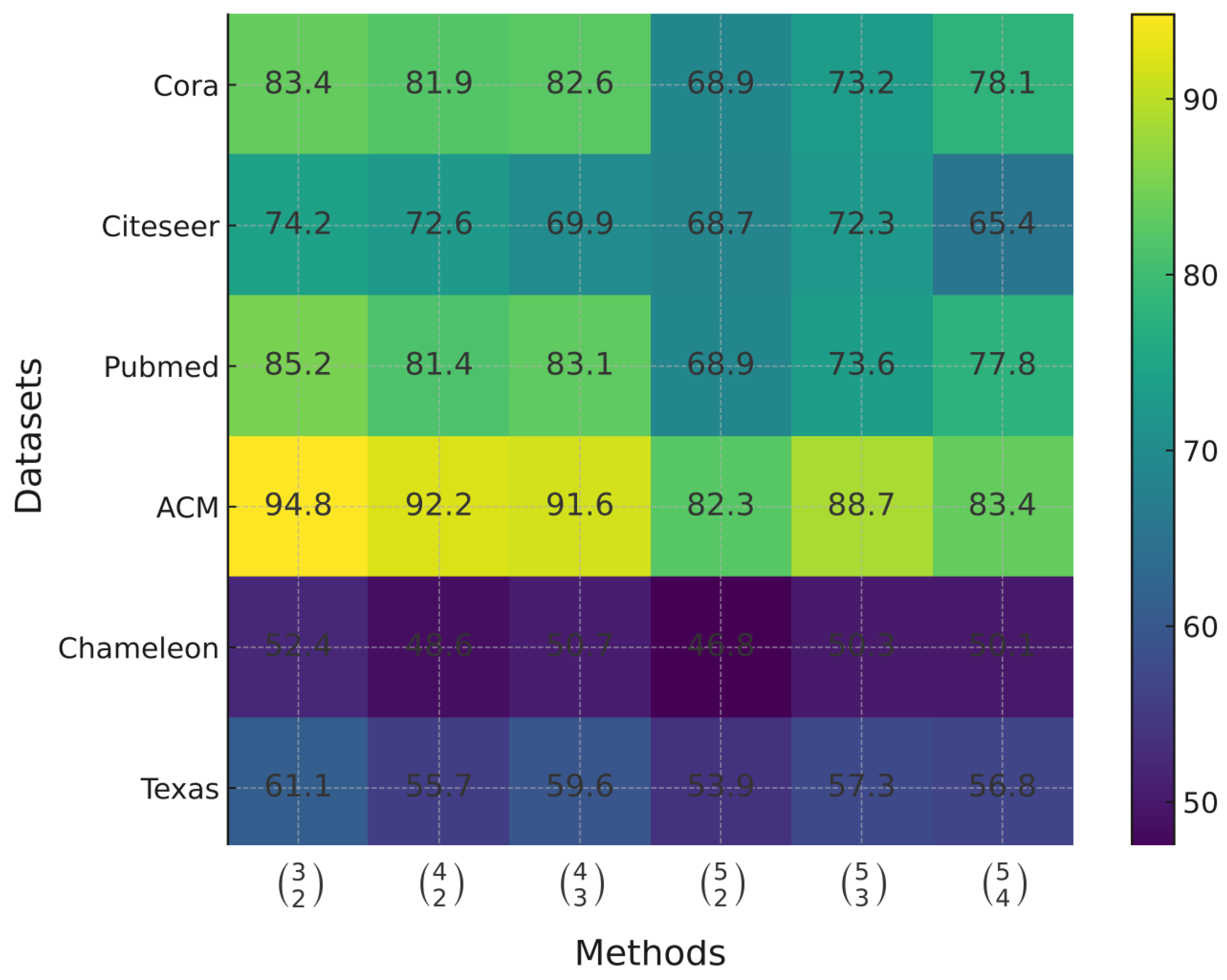
The experimental results presented in Table 9 reveal several important observations. The manual fusion setting, yields the lowest accuracy across all datasets, indicating that fixed integration schemes fail to capture the complementary information among views effectively. The random selection strategy shows only marginal improvement, suggesting that arbitrary integrations of views can not guarantee consistent information gain. The variants using only the entropy-balance or only the structural-difference term both lead to moderate performance gains, implying that each component contributes partially to the overall fusion objective. The greedy-by-entropy approach achieves slightly higher accuracy, demonstrating that prioritizing informative views provides a limited but noticeable benefit. The full optimized fusion mechanism achieves the highest accuracy across datasets, confirming that jointly considering entropy balance and structural complementarity enables more adaptive and synergistic view integration. Overall, the results validate the necessity of automatic strategy selection in promoting balanced and effective multi-view fusion.

4.4. Robustness Analysis (Q4)

As both the unsupervised ($\mathbf{OURS}-\mathbf{UN}$) and semi-supervised ($\mathbf{OURS}$) variants of VF-GRFN employ an identical fusion framework, only the semi-supervised model ($\mathbf{OURS}$), which demonstrates superior performance, is utilized in the subsequent experiments to streamline the analysis.

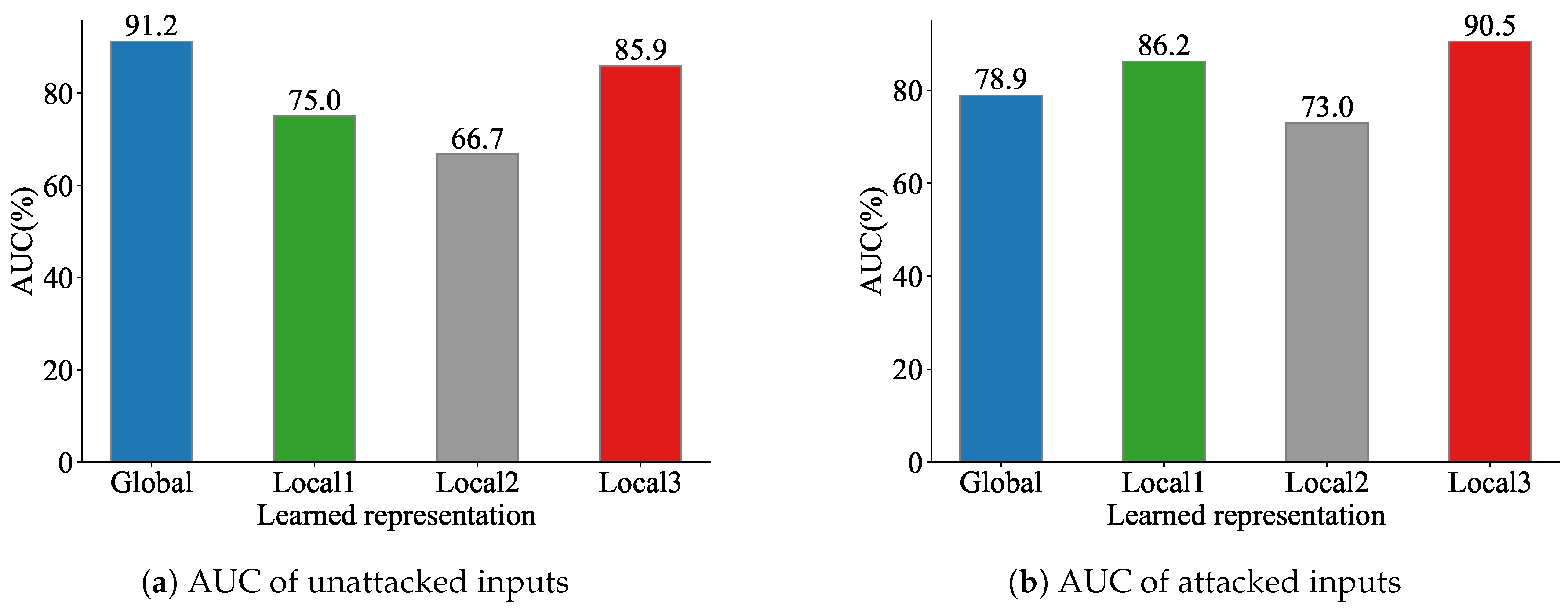
First, we evaluate the expressive capability of each view through visualization and graph reconstruction techniques.To accomplish the reconstruction of the latent representations derived from each view-specific encoder on the Cora dataset, we utilize a Variational Graph Auto-Encoder (VGAE) [34]. 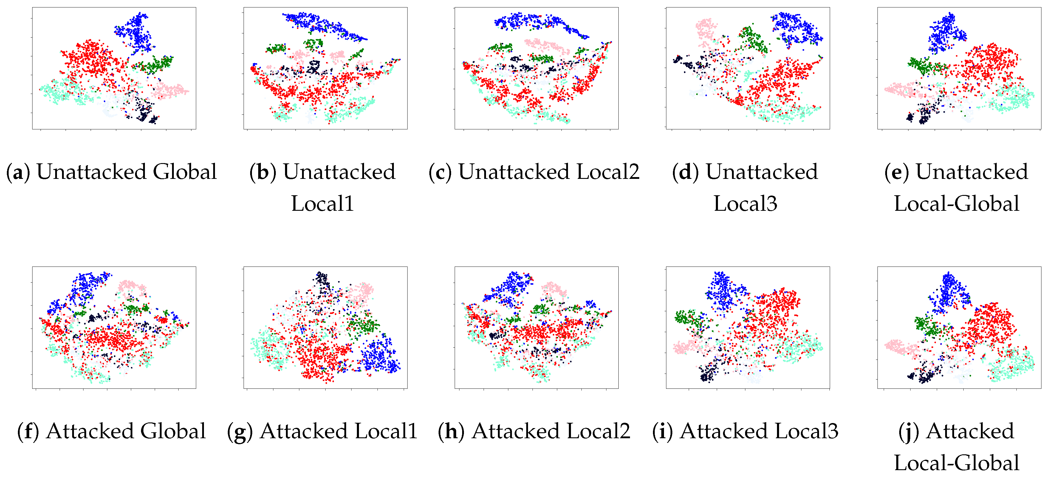The reconstruction quality is quantified using the AUC (area under the ROC curve) metric, and the corresponding results are illustrated in Figure 5. Furthermore, to intuitively demonstrate the distribution of the learned representations, we visualize the embeddings of each view encoder using t-SNE [58], as shown in Figure 6.

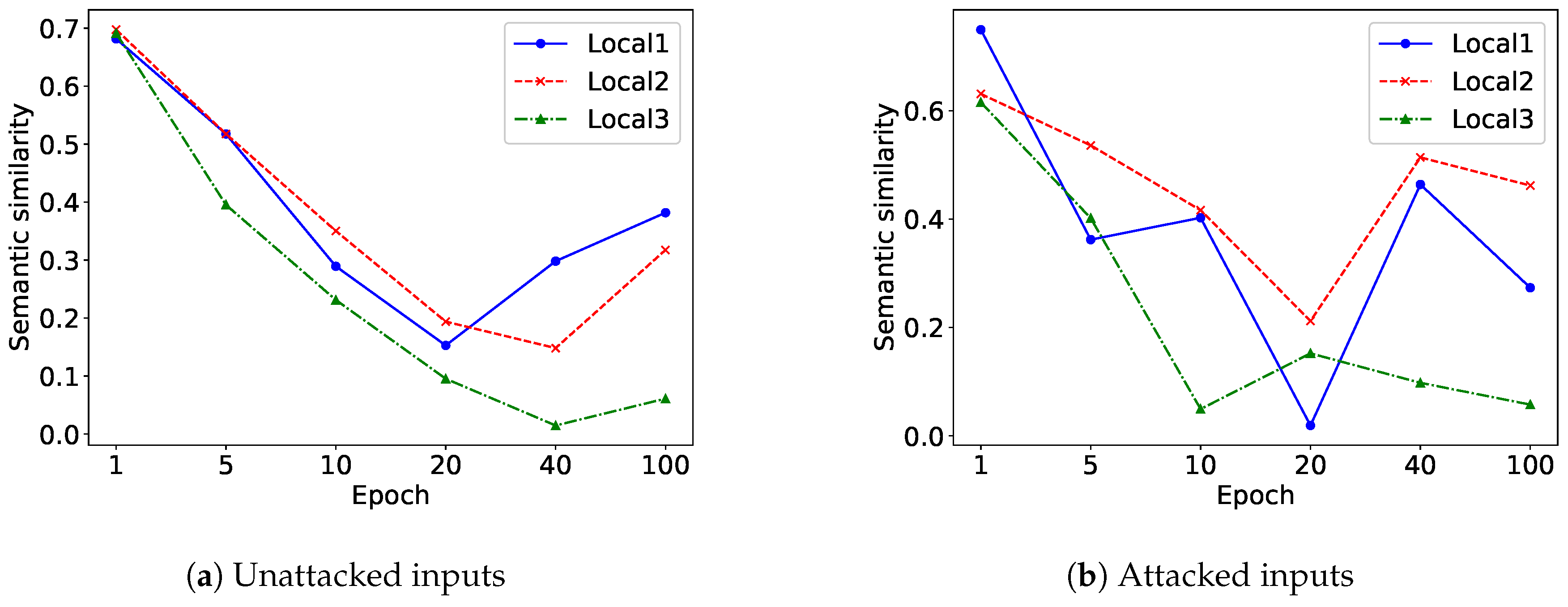
On the Cora benchmark, we monitor the evolution of semantic similarity across embeddings from the global and local views throughout the learning process. This is presented through a line-based visualization computed at selected training epochs{1; 5; 10; 20; 40; 100}. The embedding vectors for all views are obtained through the same GCN encoder. Their semantic similarity is subsequently quantified by analyzing the resulting feature representations, as depicted in Figure 7. Table 4 shows various views’ description. When the input graphs are perturbed, the expressive capability of each view encoder declines as both its visual distribution and its reconstruction quality deteriorate. In contrast, the fused representation that integrates local and global views preserves stronger expressiveness under noisy conditions, indicating that ViFi is more robust. The global-only representation performs less effectively, while local views exhibit higher discriminability and better adaptation to structural noise. Moreover, the semantic discrepancy between local and global representations grows with the proposed contrastive loss ${\mathcal{L}}_c$, confirming the significance of introducing local views. Our objective is enabled to enhance diversity among encoders from different views while maintaining the strong learning ability of key encoders. However, this divergence does not continually increase with training epochs, as the optimization is jointly constrained by contrastive and objective losses.

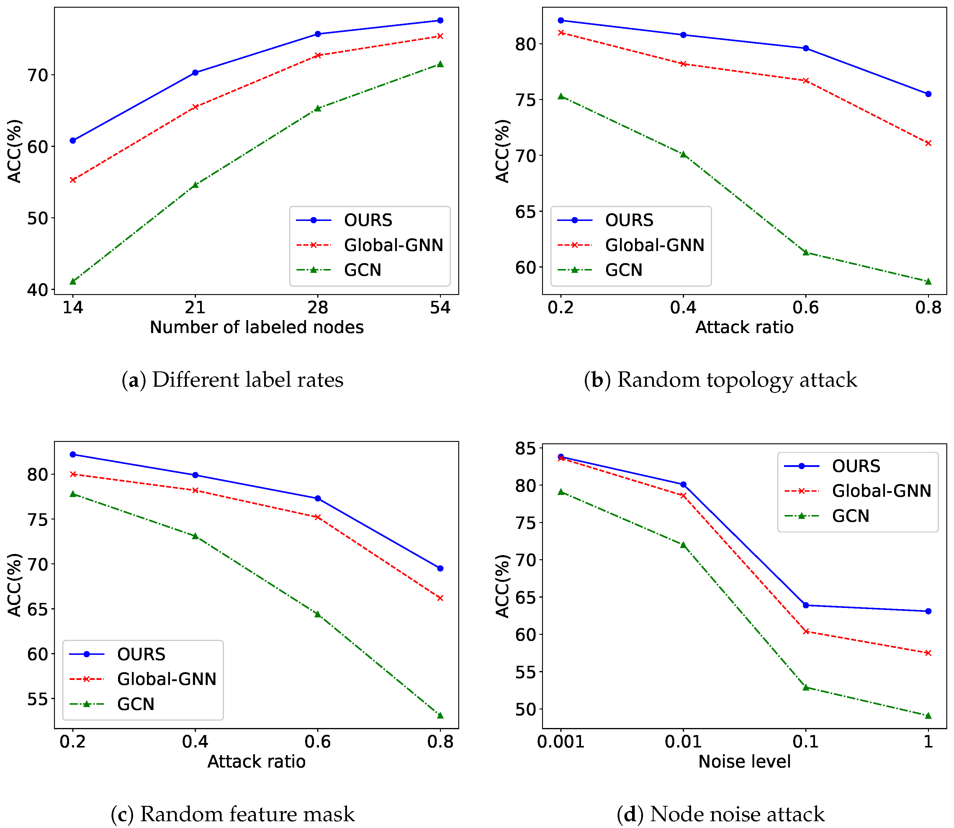
To assess the robustness of ViFi, we further subject ViFi, its variants Global-GNN, and GCN [33] to a set of four uncertainty scenarios. These conditions are used to examine how reliably each model maintains classification performance when exposed to varying views.These uncertainties may introduce disturbances to the graph structure or node semantics, thereby affecting classification accuracy. All experiments are conducted on the Cora dataset. The number of labeled nodes is set to {14; 21; 28; 54}. The attack and mask ratios are {0.2; 0.4; 0.6; 0.8}, and the noise level is adjusted to {0.001; 0.01; 0.1; 1}. For topology and feature masking, we randomly remove a portion of edges or node features according to the specified ratio. The modified graphs are then used to test classification performance on the corrupted data. In the case of feature corruption caused by node noise, we perturb the input attributes by injecting Gaussian disturbances, where the parameter noise level controls the strength of the added variation. This process intentionally distorts the original feature distribution to evaluate model stability under corrupted inputs. The corresponding outcomes are presented in Figure 8. Drawing from these observations, several key findings can be outlined as follows.

(1)

As illustrated in Figure 8(a), the baseline model experiences a sharp decline in performance as the label rate decreases. In contrast, OURS maintains superior accuracy even under extremely low label availability. This observation indicates that the introduction of a view filter and an optimized fusion mechanism enhances the model’s ability to capture essential features under limited supervision. Notably, OURS substantially outperforms Global-GNN in such low-label scenarios, further validating the effectiveness of the proposed design.

(2)

As illustrated in Figure 8(b), OURS consistently achieves superior performance compared to the baseline models under higher attack ratios. This advantage arises from its ability to effectively capture information from entropy-based view filter. In general, all methods exhibit a sharp decline in performance as the random attack ratio increases.

(3)

In alignment with earlier findings, the results presented in Figure 8(c)–(d) indicate that OURS maintains a clear advantage over both GCN and Global-GNN across varying noise and masking conditions. Overall, as the proportion of masked features or the strength of the injected noise increases, every method exhibits a substantial reduction in predictive accuracy.

4.5. Performance on Node Clustering (Q5)

We further examine the capability of the framework in unsupervised graph representation learning. Once the model is trained, the fused node representations ${\mathbf{H}}^{\left(1\right)}$ are extracted and subsequently grouped using the K-means clustering procedure on three benchmark datasets—Cora, Citeseer, and Pubmed. The evaluation is based on two metrics, normalized mutual information (NMI) and adjusted rand index (ARI), and their mean values along with standard errors are reported in Table 10. To establish competitive baselines, we incorporate a range of widely used unsupervised and contrastive graph learning methods, such as K-means, DeepWalk [53], GraphCL [50], IGCL [51], GCA [52], GAE [34], and VGAE [34]. To further illustrate the flexibility of the ViFi framework, the objective ${\mathcal{L}}_o$ is equipped with alternative contrastive components by substituting its $\mathcal{I}$ term with the loss formulations of GCA [52], IGCL [51], and GraphCL [50]. These variants are referred to as $\mathbf{OURS}$, $\mathbf{OURS}\left(\mathbf{GraphCL}\right)$, and $\mathbf{OURS}\left(\mathbf{IGCL}\right)$, respectively. Experimental results indicate that ViFi achieves performance comparable to other state-of-the-art methods across most datasets. These results confirm that ViFi exhibits strong competitiveness in unsupervised clustering tasks. Furthermore, the model’s performance is highly sensitive to the choice of $\mathcal{I}$ loss, underscoring its inherent flexibility.

4.6. Parameter Sensitivity (Q6)

Sensitivity studies are conducted on the key hyperparameters to examine their influence on model performance. ViFi is trained with $\alpha$ values ranging from 0.05 to 0.95, with an interval of 0.05. Experimental observations indicate that $\alpha$ values between 0.3 and 0.7 produce the most favorable outcomes, suggesting that maintaining a balanced emphasis between feature entropy and structural entropy enables the model to effectively capture both semantic richness and topological diversity, thereby achieving more comprehensive and discriminative representations. ViFi is trained with $\mu$ values ranging from 0.01 to 0.5, with an interval of 0.01. Experimental results show that moderate $\mu$ values, typically between 0.1 and 0.3, yield the best performance, suggesting that an appropriate regularization strength helps balance the trade-off between maximizing information gain and controlling the size of selected view subsets, thereby preventing overfitting to irrelevant views while maintaining informative diversity. We train ViFi with $\eta$ values from 0.05 to 0.95 and observe that 0.4–0.8 yields the best performance, indicating that appropriately weighting cross-encoder representation relationships improves the model.

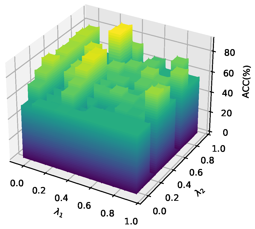
Furthermore, we investigate the effects of the hyperparameters ${\lambda }_1$ and ${\lambda }_2$ on the model’s performance. In this experiment, other hyperparameters fixed while ${\lambda }_1$ and ${\lambda }_2$ vary from 0 to 0.9. The classification results of all nodes are visualized in a 3D bar chart, as shown in Figure 9. The findings reveal that higher values of ${\lambda }_1$ and ${\lambda }_2$ generally lead to improved self-supervised learning performance.

5. Conclusion

In this paper, we proposed a novel multi-view representation learning framework called the View Filter-driven Graph Representation Fusion Network (ViFi). Following the " less for better " principle, ViFi aims to obtain more effective graph representations by leveraging fewer but more informative views. The framework first evaluates the feature–topology entropy of each view to measure its information quality, adaptively filtering those that provide complementary signals. It then integrates the filtered views through an information gain function that balances information diversity and structural consistency, ensuring collaborative and complementary fusion. Extensive experiments on classification and clustering tasks verified the effectiveness and superior performance of the proposed ViFi.

Despite the promising results, ViFi still has several limitations. The current entropy estimation relies on predefined statistical formulations, which may not fully capture higher-order correlations or latent semantic dependencies among views. Moreover, the fusion process is optimized based on pairwise information gain, potentially overlooking more complex multi-view interactions that could further enhance representation quality. Future work will explore learnable entropy modeling and more flexible fusion mechanism to better capture inter-view dependencies and improve the generalization of the framework.

References

- Xiao, S.; Li, J.; Lu, J.; et al. Graph neural networks for multi-view learning: a taxonomic review. Artificial Intelligence Review 2024, 57, 341. [Google Scholar] [CrossRef]
- Bi, J.; Dornaika, F. Sample-weighted fused graph-based semi-supervised learning on multi-view data. Information Fusion 2024, 104, 102175. [Google Scholar] [CrossRef]
- Hong, Y.; Lin, C.; Du, Y.; et al. 3d concept learning and reasoning from multi-view images. In Proceedings of the IEEE/CVF Conference on Computer Vision and Pattern Recognition, 2023; pp. 9202–9212.
- Ma, Z.; Luo, M.; Guo, H.; et al. Event-radar: Event-driven multi-view learning for multimodal fake news detection. In Proceedings of the 62nd Annual Meeting of the Association for Computational Linguistics, 2024; Vol. 1, pp. 5809–5821.
- Tian, X.; Deng, Z.; Ying, W.; et al. Deep multi-view feature learning for EEG-based epileptic seizure detection. IEEE Transactions on Neural Systems and Rehabilitation Engineering 2019, 27, 1962–1972. [Google Scholar] [CrossRef]
- Brynte, L.; Iglesias, J.P.; Olsson, C.; et al. Learning structure-from-motion with graph attention networks. In Proceedings of the IEEE/CVF Conference on Computer Vision and Pattern Recognition, 2024, pp. pp. 4808–4817.
- Cong, H.; Yang, X.; Liu, K.; et al. Feature-topology cascade perturbation for graph neural network. Engineering Applications of Artificial Intelligence 2025, 152, 110657. [Google Scholar] [CrossRef]
- Dai, S.; Wang, J.; Huang, C.; et al. Dynamic multi-view graph neural networks for citywide traffic inference. ACM Transactions on Knowledge Discovery from Data 2023, 17, 1–22. [Google Scholar] [CrossRef]
- Wang, D.; Zhang, X.; Yin, Y.; et al. Multi-view enhanced graph attention network for session-based music recommendation. ACM Transactions on Information Systems 2023, 42, 1–30. [Google Scholar] [CrossRef]
- Song, N.; Du, S.; Wu, Z.; et al. GAF-Net: Graph attention fusion network for multi-view semi-supervised classification. Expert Systems with Applications 2024, 238, 122151. [Google Scholar] [CrossRef]
- Xiong, L.; Yuan, X.; Hu, Z.; et al. Gated fusion adaptive graph neural network for urban road traffic flow prediction. Neural Processing Letters 2024, 56, 9. [Google Scholar] [CrossRef]
- Li, C.; Zhu, X.; Yan, Y.; et al. Mhgnn: Multi-view fusion based heterogeneous graph neural network. Applied Intelligence 2024, 54, 8073–8091. [Google Scholar] [CrossRef]
- Zhang, S.; Liu, J.; Jiao, Y.; et al. A Multimodal Semantic Fusion Network with Cross-Modal Alignment for Multimodal Sentiment Analysis. ACM Transactions on Multimedia Computing, Communications and Applications 2025. [Google Scholar] [CrossRef]
- Tsai, D.Y.; Lee, Y.; Matsuyama, E. Information entropy measure for evaluation of image quality. Journal of Digital Imaging 2008, 21, 338–347. [Google Scholar] [CrossRef]
- Luo, G.; Li, J.; Peng, H.; et al. Graph Entropy Guided Node Embedding Dimension Selection for Graph Neural Networks. In Proceedings of the Thirtieth International Joint Conference on Artificial Intelligence, 2021; pp. 2767–2774.
- Zhao, J.; Xie, X.; Xu, X.; Sun, S. Multi-view learning overview: Recent progress and new challenges. Information Fusion 2017, 38, 43–54. [Google Scholar] [CrossRef]
- Ma, F.; Meng, D.; Dong, X.; et al. Self-paced multi-view co-training. Journal of Machine Learning Research 2020, 21, 1–38. [Google Scholar]
- Chen, X.; Yuan, Y.; Zeng, G.; et al. Semi-supervised semantic segmentation with cross pseudo supervision. In Proceedings of the IEEE/CVF conference on Computer Vision and Pattern Recognition, 2021; pp. 2613–2622.
- Hwang, H.; Kim, G.H.; Hong, S.; et al. Multi-view representation learning via total correlation objective. Advances in Neural Information Processing Systems 2021, 34, 12194–12207. [Google Scholar]
- Niu, Y.; Shang, Y.; Tian, Y. Multi-view SVM classification with feature selection. Procedia Computer Science 2019, 162, 405–412. [Google Scholar] [CrossRef]
- Xu, R.; Wang, H. Multi-view learning with privileged weighted twin support vector machine. Expert Systems with Applications 2022, 206, 117787. [Google Scholar] [CrossRef]
- Qiao, S.; Shen, W.; Zhang, Z.; et al. Deep co-training for semi-supervised image recognition. In Proceedings of the European Conference on Computer Vision, 2018; pp. 135–152.
- Wang, W.; Arora, R.; Livescu, K.; et al. On deep multi-view representation learning. In Proceedings of the International Conference on Machine Learning; 2015; pp. 1083–1092. [Google Scholar]
- Mao, L.; Sun, S. Soft margin consistency based scalable multi-view maximum entropy discrimination. In Proceedings of the International Joint Conference on Artificial Intelligence; 2016; pp. 1839–1845. [Google Scholar]
- Yu, Z.; Dong, Z.; Yu, C.; et al. A review on multi-view learning. Frontiers of Computer Science 2025, 19, 197334. [Google Scholar] [CrossRef]
- Kachole, S.; Huang, X.; Naeini, F.B.; et al. Bimodal SegNet: Fused instance segmentation using events and RGB frames. Pattern Recognition 2024, 149, 110215. [Google Scholar] [CrossRef]
- Wei, X.; Yu, R.; Sun, J. analysis. In Proceedings of the IEEE/CVF Conference on Computer Vision and Pattern Recognition, 2020; pp. 1850–1859.
- Liang, T.; Xie, H.; Yu, K.; et al. BEVFusion: A Simple and Robust LiDAR-Camera Fusion Framework. In Proceedings of the Advances in Neural Information Processing Systems, Vol. 35; 2022; pp. 10421–10434. [Google Scholar]
- Simonyan, K.; Zisserman, A. Two-stream convolutional networks for action recognition in videos. Advances in Neural Information Processing Systems 2014, 27. [Google Scholar]
- Su, B.; Wang, W.; Lin, X.; Liu, S.; Huang, X. Identifying the potential miRNA biomarkers based on multi-view networks and reinforcement learning for diseases. Briefings in Bioinformatics 2024, 25, bbad427. [Google Scholar] [CrossRef]
- Wang, S.; Du, Y.; Zhao, S.; et al. Research on the construction of weaponry indicator system and intelligent evaluation methods. Scientific Reports 2023, 13, 19370. [Google Scholar] [CrossRef] [PubMed]
- Guo, Q.; Yang, X.; Li, M.; et al. Collaborative graph neural networks for augmented graphs: A local-to-global perspective. Pattern Recognition 2025, 158, 111020. [Google Scholar] [CrossRef]
- Kipf, T.N.; Welling, M. Semi-Supervised Classification with Graph Convolutional Networks. In Proceedings of the 5th International Conference on Learning Representations; 2017. [Google Scholar]
- Kipf, T.N.; Welling, M. Variational Graph Auto-Encoders. Computing Research Repository 2016. [Google Scholar] [CrossRef]
- Velickovic, P.; Cucurull, G.; Casanova, A.; et al. Graph Attention Networks. In Proceedings of the 6th International Conference on Learning Representations; 2018. [Google Scholar]
- Yao, K.; Liang, J.; Liang, J.; et al. Multi-view graph convolutional networks with attention mechanism. Artificial Intelligence 2022, 307, 103708. [Google Scholar] [CrossRef]
- Jin, T.; Dai, H.; Cao, L.; et al. Deepwalk-aware graph convolutional networks. Science China Information Sciences 2022, 65, 1–15. [Google Scholar] [CrossRef]
- Guo, Q.; Yang, X.; Zhang, F.; et al. Perturbation-augmented Graph Convolutional Networks: A Graph Contrastive Learning architecture for effective node classification tasks. Engineering Applications of Artificial Intelligence 2024, 129, 107616. [Google Scholar] [CrossRef]
- Abu-El-Haija, S.; Perozzi, B.; Kapoor, A.; et al. MixHop: Higher-Order Graph Convolutional Architectures via Sparsified Neighborhood Mixing. In Proceedings of the Proceedings of the 36th International Conference on Machine Learning; 2019. [Google Scholar]
- Abu-El-Haija, S.; Kapoor, A.; Perozzi, B.; et al. N-GCN: Multi-scale Graph Convolution for Semi-supervised Node Classification. In Proceedings of the 35th Conference on Uncertainty in Artificial Intelligence; 2019. [Google Scholar]
- Wang, J.; Liang, J.; Cui, J.; et al. Semi-supervised learning with mixed-order graph convolutional networks. Information Sciences 2021, 573, 171–181. [Google Scholar] [CrossRef]
- Zhang, J.; Li, M.; Xu, Y.; et al. StrucGCN: Structural enhanced graph convolutional networks for graph embedding. Information Fusion 2025, 117, 102893. [Google Scholar] [CrossRef]
- Liu, S.; He, D.; Yu, Z.; et al. Beyond homophily: Neighborhood distribution-guided graph convolutional networks. Expert Systems with Applications 2025, 259, 125274. [Google Scholar] [CrossRef]
- Li, S.; Li, W.T.; Wang, W. Co-GCN for multi-view semi-supervised learning. In Proceedings of the AAAI Conference on Artificial Intelligence, 2020, Vol. Vol. 34, pp. 4914–4698.
- Chen, Z.; Fu, L.; Yao, J.; et al. Learnable graph convolutional network and feature fusion for multi-view learning. Information Fusion 2023, 95, 109–119. [Google Scholar] [CrossRef]
- Teng, Q.; Yang, X.; Sun, Q.; et al. Sequential attention layer-wise fusion network for multi-view classification. International Journal of Machine Learning and Cybernetics 2024, 15, 5549–5561. [Google Scholar] [CrossRef]
- Wang, S.; Huang, S.; Wu, Z.; et al. Heterogeneous graph convolutional network for multi-view semi-supervised classification. Neural Networks 2024, 178, 106438. [Google Scholar] [CrossRef] [PubMed]
- Chen, Z.; Fu, L.; Xiao, S.; et al. Multi-view graph convolutional networks with differentiable node selection. ACM Transactions on Knowledge Discovery from Data 2023, 18, 1–21. [Google Scholar] [CrossRef]
- Shen, X.; Sun, D.; Pan, S.; et al. Neighbor Contrastive Learning on Learnable Graph Augmentation. In Proceedings of the 37th AAAI Conference on Artificial Intelligence, 2023; pp. 9782–9791.
- You, Y.; Chen, T.; Sui, Y.; et al. Graph Contrastive Learning with Augmentations. In Proceedings of the 33rd Annual Conference on Neural Information Processing Systems; 2020. [Google Scholar]
- Liang, H.; Du, X.; Zhu, B.; et al. Graph contrastive learning with implicit augmentations. Neural Networks 2023, 163, 156–164. [Google Scholar] [CrossRef]
- Zhu, Y.; Xu, Y.; Yu, F.; et al. Graph Contrastive Learning with Adaptive Augmentation. In Proceedings of the Proceedings of The Web Conference; 2021. [Google Scholar]
- Perozzi, B.; Al-Rfou, R.; Skiena, S. DeepWalk: online learning of social representations. In Proceedings of the 20th ACM SIGKDD International Conference on Knowledge Discovery and Data Mining; 2022. [Google Scholar]
- Kingma, D.P.; Ba, J. Adam: A Method for Stochastic Optimization. In Proceedings of the 3rd International Conference on Learning Representations; 2015. [Google Scholar]
- Strehl, A.; Ghosh, J. Cluster ensembles—a knowledge reuse framework for combining multiple partitions. Journal of Machine Learning Research 2002, 3, 583–617. [Google Scholar]
- Hubert, L.; Arabie, P. Comparing partitions. Journal of Classification 1985, 2, 193–218. [Google Scholar] [CrossRef]
- Liu, S.; Ying, R.; Dong, H.; et al. . Local Augmentation for Graph Neural Networks. In Proceedings of the International Conference on Machine Learning; 2022. [Google Scholar]
- Wang, X.; Zhu, M.; Bo, D.; et al. AM-GCN: Adaptive Multi-channel Graph Convolutional Networks. In Proceedings of the 26th ACM SIGKDD Conference on Knowledge Discovery and Data Mining; 2020. [Google Scholar]
Figure 1.
Validating the necessity of view filtering. As the number of views increases, the classification accuracy (ACC%) reaches a peak and subsequently declines, indicating that not all views contribute positively to model performance.
Figure 2.
The framework of ViFi, where modules (a) and (b) represent the core components.
Figure 3.
Heatmap of classification accuracy (ACC%) across six datasets and six view integration strategies . Brighter cells indicate higher accuracy.These patterns indicate that varying integration strategies lead to significant differences in classification performance.
Figure 4.
Comparison of classification accuracy and semantic similarity across iterations for RawC, PR, and PC.
Figure 5.
VGAE graph reconstruction performance on Cora across views. (a) AUC for unattacked inputs (learned from original views). (b) AUC for attacked inputs (learned from views with 80% edges randomly deleted).
Figure 6.
Visualization of learned embeddings on Cora across views. Unattacked (a-e): from original views. Attacked (f-j): from views with 80% edges randomly deleted.
Figure 7.
Semantic similarity between local and global view embeddings on Cora. (a) Unattacked inputs (from original views). (b) Attacked inputs (from views with 80% edges randomly removed).
Figure 8.
Performance Comparison of GCN, Global-GNN, and OURS on Cora. (a) Different label rates. (b) Random topology attack. (c) Random feature mask. (d) Node noise attack.
Figure 9.
Impact of hyperparameters and on OURS-UN’s node classification accuracy (ACC%).