Submitted:
28 November 2025
Posted:
01 December 2025
You are already at the latest version
Abstract
The global financial crises of 2008 and COVID-19 triggered market volatility, disrupting trade and foreign direct investment (FDI) flows, and impacting financial integration among economies. This study investigates the degree of financial integration between India and selected global economies—US, UK, China, Hong Kong, and Japan—during crises, using daily closing stock index data from January 2002 to June 2022. Econometric tools, including the Johansen Co-integration Test, Granger Causality Test, and Augmented Dickey-Fuller Unit Root Test, are applied to analyse short- and long-term financial linkages. The Johansen Co-integration Test results reveal long-term integration among all economies, with significant co-integrating equations detected (Trace Statistic = 98.18, Max-Eigen Statistic = 35.37) during the post-COVID period. However, the Granger Causality Test shows fluctuating short-term causal relationships, particularly with India and China shifting from bi-directional to uni-directional causality post-COVID. Standard deviations across indices, such as China (1.73) and India (1.51), highlight market volatility. The correlation matrix reveals a high correlation between India and the US (0.93 pre-COVID, 0.98 post-COVID), indicating limited opportunities for portfolio diversification. The results emphasise that sustained financial integration reduces diversification benefits and increases the potential for volatility spillovers during crises. Policymakers must identify highly connected markets and implement risk mitigation strategies to avoid systemic shocks. This study offers actionable insights for investors to navigate interconnected markets during turbulent times and provides guidance for future policy frameworks to enhance financial stability.
Keywords:
co-integration
; causality
; volatility
; diversification and global economies
Introduction
Stock market integration is one of the most crucial and widely studied phenomena in financial markets (Patel et al., 2022). The concept emerged during the 1980s and 1990s, when trade barriers were lifted, and capital controls were eased, facilitating cross-border capital flows, increasing investment opportunities, and leading to financial globalisation (Irwin, 2024). This globalisation brought lower capital costs, enhanced savings, increased profits from international diversification, and improved risk-sharing among nations (Bhanumurthy and Kumawat, 2020). Financial integration enables the linkage of domestic stock indices with global markets to maximise profits and mitigate risks. A notable outcome of India’s economic integration has been the listing of Indian shares on the US stock market, attracting international investments (Wu, 2020).
Despite the benefits of integration, volatility across interconnected stock markets can undermine the advantages of portfolio diversification. The Efficient Market Hypothesis suggests that stock prices reflect all available information, and market changes in one region should not systematically affect others. However, market linkages have grown through advancements in technology, multinational corporations, easing of exchange policies, and international capital flows (Panda, 2020). This interconnection can lead to co-integration, where markets follow shared trends or react to common external shocks. Co-integrated markets experience greater volatility spillovers, limiting the potential for diversification (Yousaf et al., 2020) and increasing susceptibility to financial crises through information leaks, volatility transmission, and news dissemination (Araya et al., 2022).
Several major crises have tested the resilience of global financial integration, including the 1987 US stock market crash, the 1997 Asian financial crisis, the 2008 global financial crisis, the 2015 Chinese market turmoil, and the COVID-19 pandemic. These events revealed the vulnerability of financial systems and led researchers to explore how crises reshape financial integration (Kolte et al., 2021). The impact of such crises varies, with developed countries often experiencing a reduction in integration, while emerging economies exhibit stronger co-movements (Lehkonen, 2014). For example, Wang (2014) demonstrated that the 2008 crisis strengthened the ties between East Asian markets and the US. These findings highlight the importance of understanding how market connections evolve during crises and the role of financial policies in shaping these dynamics.
India’s financial policies have also introduced volatility, as seen during the demonetisation of the Indian rupee in 2016. The abrupt invalidation of high-denomination notes caused short-term market panic, a 3% depreciation of the rupee against the US dollar, and a decline in investor optimism (Uke, 2017). Lahiri (2020) found that although demonetisation aimed to curb black money, it only partially achieved this goal, with significant short-term disruptions in financial markets. Similarly, global crises, such as COVID-19, had far-reaching economic implications. The pandemic not only caused a sharp decline in stock prices worldwide but also disrupted supply chains and financial stability due to China’s trade ties with developed and emerging economies. Studies by Baker et al. (2020) and Sun et al. (2021) found that COVID-19 induced significant market volatility, while Bhardwaj et al. (2022) observed weakened economic integration across markets during the pandemic.
Given the increasing interconnectedness of global economies through trade, capital flows, and regional blocs, crises originating in one region often spill over to others, causing widespread economic disruptions. This study aims to address several critical questions: What factors cause financial crises to emerge? How do crises impact financial integration among economies? Do markets strengthen or weaken their connections in response to crises? By analysing financial integration through pre- and post-crisis phases, this paper seeks to uncover patterns of convergence and divergence among key economies.
The findings of this study will provide valuable insights for policymakers and investors. Policymakers can use these insights to identify markets closely connected to India and devise strategies to mitigate risks. For investors, understanding the time horizons over which integration persists can inform diversification strategies and portfolio management. This study thus contributes to the growing literature on financial integration by exploring how crises reshape market dynamics and offering actionable recommendations for enhancing financial stability in an interconnected world.
2.0. Research Design
2.1. Statement of Problem
The interactions and integrations between global capital markets are essential for understanding portfolio diversification strategies. Historical evidence shows that volatility spillovers can trigger financial crises, transmitting financial shocks across interconnected markets. With growing financial integration, particularly among emerging economies like India, understanding these dynamics during economic turmoil becomes crucial. This study focuses on the impact of financial crises—specifically the 2008 global crisis and COVID-19—on stock market integration between selected economies. By analysing financial linkages across multiple timeframes, the study aims to evaluate whether crises weaken or strengthen financial integration. The findings will provide insights to support market participants, policymakers, and central banks in formulating strategies for economic stability and portfolio risk management.
The study aims to answer the following research questions:
- What is the degree of association and integration among selected economies during pre- and post-crisis periods?
- How do markets respond to crises, and what is the impact of these responses on financial integration?
- Does financial integration decline after crises or strengthen further?
This multifaceted problem highlights the significance of co-integration—a long-term equilibrium between financial markets. The changes in co-integration during crises affect investment strategies, market volatility, and policy responses. Insights from this research will enhance risk diversification strategies, helping market players adapt to shifting financial conditions and policy environments.
2.2. Rationale of Study
This study evaluates the effects of the 2008 global financial crisis and COVID-19 pandemic on the financial integration of stock markets in the U.S., U.K., China, India, and Japan. These nations, selected based on their global market capitalisation (M-Cap) and GDP, play a dominant role in international trade and investment flows, contributing to both stability and vulnerability in financial markets. As shown in Table 1, these economies rank among the top 10 globally in M-Cap and GDP, underscoring their significance in the study of financial integration and contagion.
These countries were chosen due to their strong trade ties and significant capital investments worldwide, with India closely linked to the U.S., China, and U.K. through bilateral trade. This interconnectedness exposes these economies to financial vulnerabilities, particularly during crises. The study seeks to determine how these relationships evolve during crises and whether lessons from past events like the 2008 crisis have strengthened financial resilience or perpetuated systemic weaknesses.
By focusing on crisis-induced volatility and contagion effects, the study offers valuable insights for investors and policymakers. Policymakers can use these insights to align their economic policies with the financial behaviour of interconnected economies, while investors can optimise portfolio strategies based on the identified patterns of co-integration and diversification opportunities.
2.3. Objectives
The objectives of the study are as follows:
- To examine the impact of crises and turbulence on short-term causal relationships among selected economies and India.
- To investigate the effect of financial crises and turbulence on long-term financial integration across the selected economies.
- To compare and analyse the pre- and post-crisis associations of India with the selected economies.
These objectives will be achieved by employing advanced econometric techniques such as Vector Error Correction Models (VECM) and Granger causality tests. The focus will be on understanding how short- and long-term market relationships evolve in the wake of financial disruptions. Furthermore, the study will explore whether policy changes in the aftermath of these crises have led to greater economic integration or contributed to market fragmentation.
3. Research Methodology
3.1. Data and Sources
This study investigates financial integration between India and five developed economies: China, Hong Kong, Japan, the UK, and the US. The analysis uses daily closing stock indices to represent market movements:
- Shanghai SE Composite Index (China)
- Nikkei 225 (Japan)
- Hang Seng (Hong Kong)
- S&P 500 (US)
- FTSE 100 (UK)
- S&P BSE Sensex (India)
The data spans January 2002 to June 2022 and is divided into:
- Pre-Global Financial Crisis: January 2002 to 2008
- Post-Global Crisis Recovery: January 2010 to December 2019
- Post-Global Crisis Shock (Lehman phase): January 2008 to December 2009
- Pre-COVID Period: January 2002 to December 2019
- Post-COVID Period: January 2020 to June 2022
The sources of data include Yahoo Finance, Bloomberg, Wall Street Journal, and relevant stock exchange websites. Excel was used for initial data formatting, while E-Views software was used for detailed econometric analysis.
3.2. Descriptive Statistics
Descriptive statistics, including mean, maximum, minimum returns, standard deviation, skewness, and kurtosis, were computed to assess market behaviour. Logarithmic returns were used to normalise the data.
- Standard deviation reveals volatility, helping investors assess risk.
- Skewness and kurtosis indicate the asymmetry and tail thickness of returns, helping to identify unusual market behaviour.
- Jarque-Bera tests assessed the normality of the data. A p-value < 0.05 rejects the null hypothesis of normality, confirming non-normality in the dataset.
These statistics help analyse trends in volatility, compare economic performance across countries, and identify potential investment opportunities or risks.
3.3. Stationarity Tests
Stationarity is essential to avoid spurious results in time-series data. The study used two unit root tests to ensure stationarity:
1. Augmented Dickey-Fuller (ADF) Test:
Accounts for autocorrelation by introducing lag terms, suitable when error terms are correlated.
2. Phillips-Perron (PP) Test:
Non-parametric test that corrects for serial correlation without adding lagged variables. It is useful when the time series shows structural breaks.
The null hypothesis assumes non-stationarity. If the p-value is < 0.05 after first differencing, the series is considered stationary and suitable for further analysis.
3.4. Co-Integration Analysis
The study employed Johansen’s Co-Integration Test to assess long-term relationships between the selected stock indices. This test is preferred over the Engle-Granger approach as it can handle multivariate models and detect multiple co-integrating vectors.
- Trace Statistic and Maximum Eigen Statistic were used to identify the number of co-integrating equations.
- At a 5% significance level, if the test statistic exceeds the critical value, the null hypothesis of no co-integration is rejected.
- Though short-term integration is sometimes weak co-integrationsuggests long-run equilibrium relationships exist. To track how these evolve especially during crises a rolling Johansen framework with a five-year window was used. It captures shifts in structural linkages over time.
3.5. Granger Causality Test
The Granger Causality Test was applied to identify short-term predictive relationships between markets:
- Lag lengths were selected based on Akaike Information Criteria (AIC) to improve model fit.
- Null Hypothesis: X does not Granger-cause Y (X ↛ Y).
- If p < 0.05, the null hypothesis is rejected, suggesting that lagged values of one variable can predict the other.
This test helps determine unidirectional or bidirectional causal relationships, offering insights into the flow of information and market spillovers. Further in order to address the limitations of conventional Granger causality in non-stationary contexts we also employed the Toda–Yamamoto causality test. This method allows for robust inference without requiring pre-testing for co-integration, making it suitable for financial time series data.
3.6. Handling Non-Normal Data
The Jarque-Bera Test results indicated non-normality, necessitating data transformation through first differencing. Outliers were adjusted through interpolation to maintain data integrity. These transformations ensure the validity of econometric models, such as regression and co-integration tests.
3.7. Software and Tools
The study utilised E-Views software for:
- ADF and PP unit root tests
- Johansen’s Co-Integration Test
- Granger Causality Test
Initial data formatting and visualisations were performed in Excel, and AIC/BIC criteria guided lag length selection for statistical tests.
4.0. Results and Discussions
The logarithmic returns of a few chosen economies are shown in Table 2, which is used to compare economies across borders.
The pre-COVID period's average returns on stock indices indicate that returns from the UK are at their highest (0.094) and variations from the mean are at their lowest (1.25). The UK has outperformed a few other chosen international markets. Returns on investment for Hong Kong and the UK were negative. The UK saw the highest returns (0.94) during the pre-COVID era, and negative returns (-0.01) during the post-COVID period. It shows that the UK's economy is still recuperating from the considerably severe effects of COVID-19.
India has a lower average return (0.06) than the UK, mostly because of its stable capital market and rising capital inflows. High returns may also be attributed to India's recent transformation, which included enhanced trade relations, the use of new technology across most of its industries, and a steady increase in foreign direct investment (FDI). Conversely, the UK and the USA, being developed economies, experience a higher standard deviation (1.51) than India's (1.25). India has the greatest average daily returns (0.05) throughout the post-COVID period, indicating a successful post-pandemic recovery. India has seen some bullish trends with stability and low volatility in past years, making it a growing and promising market.
China's average returns have been very low (0.017), which could be related to the 2008 global financial crisis, the country's stock market volatility in 2015, and rising joblessness. Slow economic development in China is partly a result of low productivity and bad company management. Its standard deviation is also at its maximum (1.73), in addition to its low returns. High standard deviations help to explain why prices fluctuate a lot and why data is dispersed or disseminated about the mean, which encourages riskier investments. The USA (0.03), China (0.01), and Japan (0.02) all had modest but positive growth rates, indicating that their economies had recovered from the COVID-19 shocks. China has the lowest standard deviation (0.012). China managed to obtain positive growth rates and also low standard deviations, which may be attributed to its policies during the post-COVID period.
China trails Japan in terms of low returns (0.02), primarily because of its growing debt and stagnating economy. The IMF reports that the growth rate of the Japanese GDP decreased by 0.9% in 2018 compared to 1.9% in 2017 (Forbes). The stock market in Japan is riskier to invest in due to its high standard deviation of 1.59 compared to a select group of other countries. Japan's (0.02) post-pandemic growth rate was positive but modest, suggesting that the country's economy had recovered from the COVID-19 shocks.
The skewness and kurtosis of stock returns are shown by the descriptive statistics of stock returns. The skewness of a normally distributed return series should be zero, and its kurtosis value should be three. All returns, with the exception of Hong Kong, were found to be negatively skewed during the pre-COVID period in the current study, indicating that Hong Kong's market is less volatile than other chosen markets where the danger of low returns is significant. Additionally, during the post-pandemic period, Japan and Hong Kong showed positive skewness, whereas China, India, the UK, and the US showed negative skewness, showing volatility brought on by the pandemic. The distribution of kurtosis was leptokurtic and stayed high for all the countries that were chosen. Elevated kurtosis values in stock returns signify the existence of anomalies and demonstrate that investors encountered significant fluctuations throughout the research period due to worldwide financial crises, volatility in the Chinese stock market, and the demonetisation of the rupee in the Indian economy. The null hypothesis is rejected according to the Jarque-Bera (Table 3) statistics since the probability is less than 5% for every index. It is, therefore, possible to conclude that none of the stocks have a normal distribution (Table 3).

Table 3.
Result of Jarque-Bera Test.
| Pre-COVID Period | Post-COVID period | |||||||||||
| Particulars | India | China | Hong Kong | Japan | UK | USA | India | China | Hong Kong | Japan | UK | USA |
| Skewness | -0.18 | -0.35 | 0.13 | -0.66 | -0.08 | -0.43 | -0.66 | -0.52 | 0.1 | 0.15 | -0.98 | -1.05 |
| Kurtosis | 13.8 | 7.8 | 17.13 | 11.46 | 12.3 | 15.5 | 9.64 | 9.69 | 5.81 | 6.11 | 13.27 | 14.35 |
| Test Statistics | 18256.7 | 3679.03 | 3115.86 | 11438 | 13704.8 | 24500.4 | 974.39 | 977.18 | 168.88 | 208.55 | 2323.3 | 2837.02 |
| Probability | 0 | 0 | 0 | 0 | 0 | 0 | 0 | 0 | 0 | 0 | 0 | 0 |
(Source: author’s calculation).
Table 4.
Correlation matrix.
| Pre- COVID period | Post-COVID period | |||||||||||
| Country | India | China | Hong Kong | Japan | UK | USA | India | China | Hong Kong | Japan | UK | US |
| India | 1 | 0.59 | 0.9 | 0.78 | 0.88 | 0.93 | 1 | 0.71 | -0.54 | 0.87 | 0.83 | 0.96 |
| China | 1 | 0.74 | 0.47 | 0.56 | 0.44 | 1 | 0.39 | 0.82 | 0.4 | 0.76 | ||
| Hong Kong | 1 | 0.7 | 0.89 | 0.78 | 1 | 0.31 | -0.04 | 0 | ||||
| Japan | 1 | 0.85 | 0.9 | 1 | 0.69 | 0.88 | ||||||
| UK | 1 | 0.88 | 1 | 0.78 | ||||||||
| USA | 1 | 1 | ||||||||||
(Source: author’s calculation).
To study the association and degree of linkage among the economies, correlation has been examined. The global market has naturally become more integrated due to increased trade and capital mobility brought about by FDI; however, the strength of this link may be examined in the above table. India and the USA have the strongest link (0.93), showing a nearly complete positive correlation between the two markets. It is evident that the USA, India's principal commercial partner, has close ties with India. India and Hong Kong have strong ties outside the USA because of their $26 billion bilateral trade in 2017. The trade history between the two countries dates back to the 19th century when India was a significant importer and supplier of products to Hong Kong. In addition, Hong Kong facilitates the re-exporting of Indian commodities to China's mainland.
Despite China being India's biggest trading partner and importer, the correlation coefficient between the two countries' returns stayed at its lowest value of 0.59. A moderate correlation exists between the two countries, which can be explained by the Chinese stock market bubble, rising border tensions between them, and the fact that each country's share index moves in the opposite way due to its own goals and rhythm. The majority of the companies in India's share index are focused on serving local customers, or they are in industries where software exports—which are not in China's stronghold—dominate. However, the connection between China and India was found to be the lowest, opening the door for portfolio diversification as a means of reducing risk. India and the UK also have a strong additional association (0.88) Given that the UK is India's third-largest foreign investor and India is the UK's second-largest foreign investor, their relationship is solid and constructive. Tripathi and Sethi (2010) found that the Indian stock market is not integrated with the stock markets of China, Japan, and the UK, which is in contrast to Raj and Marcus's (2019) conclusion that there is a positive correlation between the stock markets of India and those of the US, Hong Kong, Japan, and China. Positive stock market integration with the US market alone was revealed by the study.
As the correlation between India and China has increased from 0.59 to 0.71 in the post-COVID period, the correlation in this period will provide insight into the impact of COVID-19 on specific economies. Trade activities may be to blame, as both economies are developing and seeking to recover from the pandemic. Nonetheless, a somewhat negative correlation between India and Hong Kong has been observed in the post-COVID era, in contrast to a strongly favorable correlation during the pre-COVID era. When two variables X and Y have a negative correlation, their movements will be counter to each other; as one increases, the other will drop. Investors frequently employ inversely correlated assets to reduce risk without having an impact on their portfolios.
India and the US have a long history of relationship, as seen by the pre-COVID time and the post-COVID era. Following the US, there is a strong association with Japan (0.87) and the UK (0.83). Strong positive correlation unequivocally demonstrates that countries are engaging in international commerce and investment. China and Japan are found to have a higher post-COVID correlation (0.82) than they have had before the COVID-19 pandemic. The two countries' growing economic ties can be attributed to their tight bilateral connections. China's exports to Japan have surged over the past 25 years, experiencing an annual growth rate of 6.3%. This growth trajectory is expected to propel exports to $157.5 billion by 2023, up from $32 billion in 1995. However, because of COVID-19, there was no correlation with the US and a negative, modest correlation (-0.04) between Hong Kong and the UK. As in the pre-COVID era, the US and Japan continue to have a high positive association (0.88). The UK and the US formerly showed a high positive association, which has persisted into the post-COVID era. Notwithstanding the epidemic, there is still a positive or negative link between the economies of the US and Hong Kong, but otherwise none at all. As the pre-condition of testing co-integration among stock indices is to examine whether all variables are stationary of the same order or not, the stationarity of all indices has been checked through the ADF unit root test. The test examines the null hypothesis that the series has no unit root and that data is stationary. To test the null hypothesis, the probability of test statistics will be compared with 0.05. The null hypothesis cannot be rejected if the probability is more than 0.05. However, if probability is less than 0.05, the null hypothesis will be rejected i.e., data will be presumed to be stationary. The test results have been reported in Table 5.
All the chosen series are non-stationary at the initial level but stationary at the first difference, as the above table makes abundantly clear. Financial variables typically exhibit upward movement over time and exhibit signs of a trend or pattern. The findings show that the null hypothesis cannot be rejected at the initial level for all indices. Put differently, every stock index exhibits non-stationarity at certain levels. However, the likelihood remains less than 0.05 following the initial differencing, indicating the absence of a unit root. Stated otherwise, it is noticed that every series is integrated into order 1. To analyze potential long-term co-integration among the chosen economies, the Johansen co-integration test has now been used at 1 lag length (as recommended by lag length criteria, AIC). Trace and Max-Eigen statistics estimates are provided by the Johansen co-integration test. The hypothesis cannot be rejected if these statistics are greater than their corresponding critical values at the 5% level of significance, and vice versa. The table below contains the results of the same (Table 6).
To investigate potential long-term links among the chosen markets, the study used Eigenvalue and Trace statistics. The co-integration test yields identical results for the pre- and post-COVID eras. At the 5% level of significance, the trace statistics and maximal Eigen statistics for both periods rule out the idea that there are no co-integrated equations among the chosen indices. Consequently, it may be said that the stock indices exhibit long-term co-integration. The existence of a co-integrating equation suggests that some stock markets are propelled by a common factor and exhibit a common trend over the long term. These factors will initially move apart greatly, but over time, some of them will return to their equilibrium paths, making it more difficult for investors to benefit from the diversity of an international portfolio. Statistics showing correlation support the findings. However, the Indian stock market did not integrate with Hong Kong or Japan over the long term. The same conclusions were reached by Kumar (2021), who noted that there was no long-term co-integration between the stock markets of China, Japan, and India. There has been long-term financial integration between the Japanese stock market and the Indian stock market. Using Johansen trace statistics, Deo and Prakash (2017) conducted an empirical investigation on the co-integration of the Indian stock market with key global stock markets, such as those in Japan, Hong Kong, China, the UK, and the USA. According to the analysis, the markets that were chosen to have long-term integration.
To evaluate the strength of long-run equilibrium relationships during the post-pandemic phase, the Johansen co- integration test was applied for the period January 2020 to July 2023 using 1 lag length as selected by AIC criteria. The test provides both Trace and Max-Eigen statistics, which determine the number of co-integrating vectors at a 5% level of significance. The null hypothesis of no co-integration is rejected when the calculated test statistics exceed the respective critical values. The results of the post-COVID co-integration analysis are presented in the following Table 6.1
The post-COVID co-integration results show the presence of four statistically significant co-integration relationships at the 5% level. This confirms that despite global uncertainty and asymmetric recovery paths across economies, the selected stock markets—including India, the US, UK, Japan, Hong Kong and China continue to share a long-run equilibrium relationship. The evidence suggests that integration did not deteriorate but rather remained robust during the post-pandemic period. As a result the opportunities for global portfolio diversification remained limited. These findings are consistent with previous research by Kumar (2021) which highlighted strong long-run integration among global markets with the exception of certain East Asian pairs.
To further validate the stability of financial integration, a rolling Johansen co-integration test was applied using 5-year (1260 trading days) moving windows. This approach helps detect whether long-run relationships persist or break over time particularly during episodes of economic distress. The Johansen framework was estimated across successive windows with a step size of 20 trading days and the number of co-integrating vectors was recorded for each window.
The following figure (Figure 1) presents the variation in co-integrating ranks over time, offering insights into the dynamic nature of global financial linkages.
The rolling co-integration analysis highlights that the number of co-integrating vectors remained consistently above three during most windows. This indicates that the structural relationship among the selected stock markets has not only persisted but also adjusted dynamically during various global events, including the 2008 financial crisis, the COVID-19 shock and recent geopolitical disruptions. These findings provide further evidence that financial markets are strongly and consistently linked in the long run. As a result, international diversification benefits may be significantly reduced particularly for Indian investors aiming to hedge using these developed markets. The results corroborate existing literature on dynamic financial integration and align with studies that emphasise time-varying but persistent global market co-movements. However, it's important to note that even when co-integrating relationships are present or evolving over time, they do not always correspond to short-term correlation patterns. For instance, despite a near-perfect post- COVID correlation between India and the US, the Johansen test detects only one co-integrating vector in that phase. This reinforces the idea that co-integration captures deeper structural links beyond transient co-movements making it essential to interpret correlation and co-integration as distinct concepts, especially when evaluating diversification strategies. Hence, diversification benefits may still exist in the absence of strong co- integration, despite high correlation. Using the Granger causality test (1969), a potential short-term link between sock markets has been investigated. The test establishes the direction of the stock market's causal relationship. The null hypothesis states that X ↛ Y, or that Country X does not Granger cause Country Y. Should the likelihood of the F-statistics be more than 0.05, the null hypothesis will be accepted. In this instance, no causality will be presumed. Nonetheless, the null hypothesis will be rejected and it will be determined that there is a causal relationship between the two stock markets if the probability of the F-statistics is less than 0.05. The Granger Causality test results are shown in the table below (Table 7).
The findings show that unidirectional causality between India and China, India and Hong Kong, and India and the UK existed throughout the pre-COVID era. The unidirectional relationship between country X and country Y merely illustrates the possibility of a crisis in country X spreading to country Y.
India is causally related to China, the United Kingdom, and Hong Kong due to its trade links, cross-border investment, and capital mobility. Despite the relatively low causality, India shares a causality of 9.64 with China, 12.49 with Hong Kong, and 20.28 with the UK, with other countries. There was also evidence of some reciprocal relationships between India, the US and Japan. As was previously said, trade relations between India and Japan are strong, with Japan ranking among India's top 5 investors. The findings show that while there is minimal short-term causality (12.33) from India to the USA, there is a significant magnitude of short-term causality (153.18) from the USA to India. The main causes of the bidirectional relationship include commerce, investment, and positive ties between the two. The findings unequivocally show that there is no opportunity for investors to diversify and profit, but there is also a substantial danger of volatility and contagion because of correlation and short-term causality among the chosen countries within the relevant time period. Joshi et al. (2021) research also discovered both unidirectional and bidirectional causality between the American and Indian stock market indices, which corroborated the findings.
There was no unidirectional or bidirectional causal relationship between the countries. There is a tiny window of opportunity for investors to diversify their portfolios and profit from these markets if there is no causal relationship between India and Hong Kong in the short term. Causality between China and India is observed to flow from China to India, whereas it was going from India to China before the COVID-19 pandemic. India and Japan have a unidirectional relationship, with causality primarily moving from India to Japan and India to the UK for commercial and investment purposes. India and the US continue to have bidirectional causality in the post-COVID era. With the exception of Hong Kong and India, every nation has some degree of causation, which explains why any oscillation in one nation would also produce turbulence in another. As a result, a risk-averse investor shouldn't select that nation to diversify their portfolio and so reduce risk.
The sample descriptive statistics (Table 8), which are a valuable tool for revealing information about the behavior of certain stock market returns before a crisis, are shown in Table 8. All markets have nearly zero daily average returns, with China having the highest (0.08), the US and Hong Kong having comparable returns (0.07), and India and the UK having the lowest (0.014). Increased commerce, a growing GDP, and rising FDI inflows may have contributed to China's high returns. India's low returns were mostly caused by huge income gaps, low household per capita income, and inequality during the 2002–2007 periods. All of the chosen economies have nearly low standard deviations, but Hong Kong has the lowest mean deviations, suggesting a minimal investment risk.
Additionally, all of the countries except the US exhibit negative skewness, suggesting that while investors may see a few little wins, there is a chance that they may also experience significant losses (Table 9). Negative skewness generally lessens the risky side of investing if it is accompanied by positive mean value or high average returns. Therefore, when deciding how much money to invest in a certain economy, skewness shouldn't be the only factor taken into account. Finally, for a distribution to have a bell-shaped curve or be normally distributed, the kurtosis value must equal 3. Since all of the countries have high kurtosis values far higher than 3, this indicates that the distribution is leptokurtic. The US, on the other hand, has the lowest value (5.89) and is closest to a mesokurtic distribution (kurtosis of 3). The above results show that the US in the pre-crisis period, had a stable market with low risk. The test stats for all the selected economies are very high indicating series is not normally distributed.
The US had the highest average returns post-crisis period (0.031), followed by Japan (0.017). Its economic policies allowed both countries to recover from their crises. China was in second place with minimum returns, while Hong Kong had negative returns (0.001). The standard deviation was highest (0.016) for China, Japan, and Hong Kong, but it was nearly identical for all other countries, suggesting instability brought on by global issues. Due to hazardous investments and losses brought on by crises that spread to all the chosen economies, all of the economies were severely distorted. Every country had a peak that exceeded Kurtosis. The US has the highest kurtosis (16.90). Test stats depict that in the post-crisis period also the series was not normally distributed as the value of test stats is very high.
The correlation matrix elucidates the association between the Indian stock market and other specific indices of global main stock exchanges (Table 10). Karl Pearson's coefficient correlation has been calculated to investigate potential relationships between the chosen economies. The findings show that, before the financial crisis, India’s correlation with all the chosen economies ranged from almost perfect to high; Hong Kong had the highest correlation (0.97), followed by the US (0.89). Reformulating and rephrasing regulations, loosening trade restrictions, globalisation, and interdependence are the causes of the high association. China has a modest relationship with Japan and a high affinity with Hong Kong. Japan, however, has a fairly strong association with the US (0.92) and the UK (0.95). Japan imports manufactured goods and raw materials from the United States. Finally, the UK and the US have a nearly flawless correlation (0.95) primarily due to trade links; in 2002, the US exports of goods to the UK were 33,204 million dollars, while imports were 40,744 million dollars. By 2003, exports had climbed to 49,981 million dollars, and imports to 56,857 million dollars. These data accurately demonstrate the relationship between the two countries.
India had a nearly perfect correlation (0.98) with the US in the post-crisis era, primarily due to trade ties, while also having a strong positive correlation (0.94) with Japan. In contrast, the US showed a strong correlation with Japan and a modest association with China, Hong Kong, and the UK. China's moderate (0.42) and low (0.34) correlations with the US and the UK can be attributed to the effects of crises on the Chinese economy. Hong Kong and the US likewise have a moderate association (0.61). According to the above table, trade and investment have continued to contribute to economic connection, though to a lesser extent. However, this correlation has remained strong and nearly perfect for the US and India despite the financial crisis (Table 11).
The present study is based on examining the short-run and long-run integration therefore, it is necessary to check for stationarity of data. The study's variables must be stationary. If they aren't, it's presumed that they contain deterministic or stochastic tendencies. The Augmented Dickey-Fuller test was used to verify stationarity. The results showed that all indices are non-stationary at the original level, with probability values greater than 0.5, but stationary at the level or first difference, with probability values less than 0.05. Therefore, the long-run co-integration among chosen economies can be examined using the co-integration test.
The study then tests the co-integrating relationship after using the Unit Root Test to verify the time series of each variable's attributes. At the 5% significance level, the values of Trace and Max-Eigen Statistics must be more than the critical value to accept the co-integrating relationship between the variables.
The trace statistics shown in Table 12 indicate the existence of co-integration in the stock indices in both the pre-and post-crisis periods, as trace statistics values are higher than critical values at none and at most 1 in the pre- crisis period and greater than the critical value at none in the post-crisis period. These are the empirical results of the co-integration rank test, which is derived from Johansen's trace test. Because the p-values are less than 0.05, the p-value statistics validate the findings. It indicates that there were two co-integrating equations or vectors in the pre-crisis period and one in the post-crisis period, rejecting the null hypothesis that there was no co-integration between stock indexes.
Granger Causality Analysis is a statistical hypothesis test that indicates the direction of the relationship between variables and assesses if one-time series data can be used to predict another (Table 13). To determine which of the two variables selected is the cause and which is the effect, the Granger Causality Test is used. It is evident that prior to the financial crisis, there was a one-way causal relationship between the US and India as well as a two-way relationship between Hong Kong and India. It merely indicates that investing in certain countries does not allow investors to profit from portfolio diversification. There is no causative relationship between India and Japan, there is only one-way causality from the UK to India. This suggests that investors have a limited window of opportunity to diversify their portfolios and gain from diversification in the near term.
Examining the post-global crisis era, we find that every economy we chose had uni- or bi-directional links; not a single economy displayed any indication of no causality. The findings indicate that investor confidence in economies has returned, and cross-border money flows and commerce have resumed. Additionally, investors are unable to diversify their portfolios because markets are still interconnected and can short-circuit one another. It is possible to observe unidirectional causality between China and India, India and Hong Kong, India and Japan, and India and the UK. India and the US were nearly completely correlated with each other, despite the fact that correlation analysis revealed bi-directional causality between them.
To further explore“post-global financial crisis recovery” window (2010–2019) was split into three phases: pre-crisis buildup (2002–2007), acute crisis (2008–2009) and recovery (2010–2019). Granger causality tests were applied between India and the US during each of these windows to track directional influences over time.
Table 13.1 explains the findings and results. During the pre-crisis window (2002–2007), the US Granger-caused Indian stock market returns significantly across both lag structures while India showed marginal causality at lag 2. Interestingly, during the peak global financial shock (2008–2009), no causality was found in either direction likely reflecting the dislocation in market linkages due to systemic stress. In the recovery window (2010–2019), US influence re-emerged significantly on Indian markets while India's predictive power diminished. These findings suggest that while financial linkages may be strong under normal or recovery conditions, they often collapse during periods of systemic global distress. This time-varying causality pattern reaffirms the need to disaggregate crisis timelines to capture transmission volatility more accurately.
While Granger causality tests are commonly used to detect predictive relationships between financial time series they do not imply true economic causation. In this study, Granger causality merely indicates whether past values of one market help forecast another. However, this statistical dependence may arise due to shared exposure to third-party shocks, such as synchronised monetary policy responses or global risk events. For example, the observed high correlation between the Indian and US markets post-COVID (0.98) may reflect common reactions to Federal Reserve policies or coordinated fiscal stimuli rather than direct transmission. These omitted or un- modelled influences could confound the detected relationships thereby calling for a more robust framework. To address these concerns, we extend the analysis using the Toda–Yamamoto causality test, which corrects for potential non-stationarity and avoids the limitations of pre-testing inherent in traditional Granger frameworks. This ensures a more reliable assessment of predictive influence in the presence of integrated variables.
Table 13. 2.
Toda–Yamamoto causality test.
| Global Crises Period | ||||
| Null Hypothesis: Y (X ↛ Y) | Chi-square Statistics | P-value | Result | Causality |
| USA ↛ India | 50.74 | 0.00 | Rejected |
Bi-directional |
| India ↛ USA | 146.89 | 0.00 | Rejected | |
(Source: author’s calculation).
To account for the limitations of Granger causality under non-stationarity, the Toda–Yamamoto test was applied between India and the US. The results confirmed bidirectional causality: while the US strongly influences the Indian market, India also shows predictive power for US market movements. This suggests that the Indian market may contain predictive signals for US market behaviour, potentially reflecting global investor sentiment or interlinked economic developments. This supports earlier findings and suggests that their high correlation is not just due to shared global shocks like Fed policies, but reflects a deeper interdependence.
5. Future Implications
The findings of this study highlight how crucial economic integration is, especially in times of crisis. Governments ought to give top priority to programs that strengthen resilience and closer economic links. Bilateral trade agreements and investment partnerships must be strengthened to lessen the impact of upcoming disruptions. Furthermore, trade diversification strategies can lessen dependency on certain markets and improve general economic stability.
These measures can provide a buffer against economic shocks for the household sector, ensuring a steady flow of goods and services even during crises. Households will benefit from greater economic stability, which can translate into more secure employment and income opportunities. Enhanced economic integration might benefit industrialists by potentially creating larger markets and stronger supply chains, which can lessen their vulnerability to localised disturbances.
According to recent trends, global economies are becoming more interdependent, and regional trade agreements and economic alliances are becoming increasingly important. For example, the Regional Comprehensive Economic Partnership (RCEP) has emphasised the advantages of wide-ranging economic cooperation. This research adds to this changing field by demonstrating the importance of persistent and proactive integration efforts.
India should increase efforts to deepen its economic ties with important allies including the US, Japan, and the UK. These alliances are essential for both strategic stability and economic progress. To ensure prompt and efficient responses to developing dynamics, authorities must be on the lookout for changes in the short-term causal relationships across economies and constantly monitor and handle them. Ultimately, overcoming obstacles and maintaining long-term prosperity and stability will require cultivating strong economic linkages and flexibility to shifting conditions.
6. Conclusion
The analysis sheds light on how economies handled crisis circumstances. India's correlation with the US, Japan, and the UK remained strong despite the COVID-19 epidemic; suggesting that trade and FDI between these countries were not significantly affected. The post-COVID analysis clarified this integration by showing how economies stayed interconnected over time. Short-term analyses highlighted that India demonstrated causal linkages with the UK, the US, Japan, and China, except for Hong Kong, and that these associations persisted during times of crisis. Similar patterns were observed during the Global Financial Crisis, with India's correlations remaining largely stable over time. The long-term economic integration and convergence were validated using the Johansen trace tests. The rolling co-integration results reinforced the presence of persistent long-term linkages, especially during crisis periods such as the post-COVID phase. These findings support the hypothesis of dynamic and evolving global financial integration. Notably, by isolating the pre- and post-Lehman periods, we observed that the India–US causality shifted from one-way to bi-directional. This suggests that severe financial shocks can restructure influence patterns and deepen inter-market ties over time. While India and the US exhibited high short- term correlation in recent years, the limited number of co-integrating vectors indicates that their long-term equilibrium relationships remain distinct. This distinction is essential for understanding deeper financial integration versus superficial market connectivity
Furthermore, post-crisis dynamics showed a bidirectional relationship between the US and India, despite a unidirectional causal relationship existing between the two countries before the global financial crisis. This change implies that, despite fewer chances for diversification, the crisis may have had a short-term positive impact on their economic connection. To reinforce this finding and address concerns of omitted variable bias—such as from global policy shocks like Federal Reserve actions—the study employed the Toda–Yamamoto causality framework alongside traditional Granger tests. This approach confirmed the robustness of the India–US bidirectional linkage with greater econometric reliability.
Interestingly, to note that causality between India and Japan did not develop until after the global financial crisis, indicating a substantial change in their economic ties. Our findings diverge from previous works, particularly those based on Tobin's portfolio theory, which posits that diversification benefits diminish during periods of high market integration. Contrary to this theory, our results indicate that economic integration did not weaken during crises—in fact, in several cases, it substantially enhanced. This shows that the complexity of contemporary financial markets, particularly in times of crisis, may go beyond the theoretical bounds of Tobin's portfolio theory. To summarise, the economies under examination demonstrated adaptability, unity, and shifting dynamics in their interconnections throughout time—even in the face of crises and shifts in policy. It can also be concluded that short-term causal links were greatly impacted by shifts in governmental policies and economic crises, although long-term integration and correlation remained rather constant. As a result, this study advances knowledge about financial integration and the forces that support it, providing investors, academics, and policymakers with insightful information.
Funding
No funds were provided by any sponsor or agency.
Data Availability Statement
Data has been taken from reliable sources and no manipulation has been done.
Acknowledgements
Not applicable.
Competing Interests
The authors declare no conflict of interest.
References
- Akhtaruzzaman, M., Boubaker, S., & Sensoy, A. (2021). Financial contagion during COVID–19 crisis. Finance Research Letters, 38, 101604. [CrossRef]
- Araya, A., Dahalan, J., & Muhammad, B. (2022). The relationship between financial patterns and exogenous variables: Empirical evidence from symmetric and asymmetric ADRL. International Journal of Business Society, 6(6), 638-661. [CrossRef]
- Baker, S. R., Bloom, N., Davis, S. J., & Terry, S. J. (2020). COVID-induced economic uncertainty (No. w26983). National Bureau of Economic Research. http://www.nber.org/papers/w26983.
- Basuony, M. A., Bouaddi, M., Ali, H., & EmadEldeen, R. (2022). The effect of COVID-19 pandemic on global stock markets: Return, volatility, and bad state probability dynamics. Journal of Public Affairs, 22, e2761. [CrossRef]
- Bhanumurthy, N. R., & Kumawat, L. (2020). Financial globalization and economic growth in South Asia. South Asia Economic Journal, 21(1), 31-57. [CrossRef]
- Bhardwaj, N., Sharma, N., & Mavi, A. K. (2022). Impact of COVID-19 on long run and short run financial integration among emerging Asian stock markets. Business, Management and Economics Engineering, 20(2), 189-206. [CrossRef]
- Chaudhary, R., Bakhshi, P., & Gupta, H. (2020). Volatility in international stock markets: An empirical study during COVID-19. Journal of Risk and Financial Management, 13(9), 208. [CrossRef]
- Deo, M., & Prakash, P. A. (2017). A Study of Integration of Stock Markets: Empirical Evidence from National Stock Exchange and Major Global Stock Markets. ICTACT Journal of Management Studies, 3(2). [CrossRef]
- Goyal, N., & Mittal, A. K. (2020). Impact of demonetization on the Indian stock market returns and volatility. https://ssrn.com/abstract=3911682.
- Guru, B. K., & Das, A. (2021). COVID-19 and uncertainty spillovers in Indian stock market. MethodsX, 8, 101199. [CrossRef]
- Irwin, D. A. (2024). Does trade reform promote economic growth? A review of recent evidence. The World Bank Research Observer, lkae003. [CrossRef]
- Izzeldin, M., Muradoğlu, Y. G., Pappas, V., & Sivaprasad, S. (2021). The impact of COVID-19 on G7 stock markets volatility: Evidence from a ST-HAR model. International Review of Financial Analysis, 74, 101671. [CrossRef]
- Jiang, Y., Yu, M., & Hashmi, S. M. (2017). The financial crisis and co-movement of global stock markets—a case of six major economies. Sustainability, 9(2), 260. [CrossRef]
- Joshi, N. A., Mehta, D., Patel, B., & Patel, N. (2021). Causality and cointegration among stock market indices: A study of developed markets with sensex. International Journal of Accounting & Finance Review, 7(1), 31-52. [CrossRef]
- Kolte, A., Roy, J. K., Patil, D. T., Pawar, A., & Sharma, P. (2021, March). Global Financial Crisis in 21st Century: A Brief Analysis of Stock Exchanges. In 2021 International Conference on Computational Intelligence and Knowledge Economy (ICCIKE) (pp. 290-295). IEEE. [CrossRef]
- Kumar, R., & Dhankar, R. S. (2017). Financial instability, integration and volatility of emerging South Asian stock markets. South Asian Journal of Business Studies, 6(2), 177-190. [CrossRef]
- Kumar, S. (2021). Long run dynamics of Indian stock market with major Asian stock markets. International Journal of Science and Research,10(8),1-4. [CrossRef]
- Lahiri, A. (2020). The great Indian demonetization. The Journal of Economic Perspectives, 34(1), 55–74. https://www.jstor.org/stable/26873529.
- Lehkonen, H. (2014). Essays on emerging financial markets, political institutions and development differences (Doctoral dissertation, University of Jyväskylä). https://jyx.jyu.fi/handle/123456789/43114.
- Panda, R. (2020). Financial Integration of Corporate Bond Markets in India: Empirical Evidences (Doctoral dissertation). http://ethesis.nitrkl.ac.in/10179/.
- Patel, R., Goodell, J. W., Oriani, M. E., Paltrinieri, A., & Yarovaya, L. (2022). A bibliometric review of financial market integration literature. International Review of Financial Analysis, 80, 102035. [CrossRef]
- Raj, G. R., & Marcus, A. (2019). Market linkage of Indian stock market with select stock markets. Economic affairs, 64(1), 185-190. [CrossRef]
- Rajwani, S., & Mukherjee. (2013). Is the Indian stock market cointegrated with other Asian markets? Management Research Review, 36(9), 899-918. [CrossRef]
- Sun, P., Wang, M., Song, T., Wu, Y., Luo, J., Chen, L., & Yan, L. (2021). The psychological impact of COVID-19 pandemic on health care workers: a systematic review and meta-analysis. Frontiers in Psychology, 12, 626547. [CrossRef]
- Tripathi, V., & Sethi, S. (2010). Integration of Indian stock market with World stock markets. Asian Journal of Business and accounting, 3(1), 117-134. https://ssrn.com/abstract=1747038.
- Uddin, M., Chowdhury, A., Anderson, K., & Chaudhuri, K. (2021). The effect of COVID–19 pandemic on global stock market volatility: Can economic strength help to manage the uncertainty?. Journal of Business Research, 128, 31-44. [CrossRef]
- Uke, L. (2017). Demonetization and its effects in India. SSRG International Journal of Economics and Management Studies, 4(2), 18-23. [CrossRef]
- Wang, L. (2014). Who moves East Asian stock markets? The role of the 2007–2009 global financial crisis. Journal of International Financial Markets, Institutions and Money, 28, 182-203. [CrossRef]
- Wu, F. (2020). Stock market integration in East and Southeast Asia: The role of global factors. International Review of Financial Analysis, 67, 101416. [CrossRef]
- Yousaf, I., Ali, S., & Wong, W. K. (2020). An empirical analysis of the volatility spillover effect between world-leading and the Asian stock markets: Implications for portfolio management. Journal of Risk and Financial Management, 13(10), 226. [CrossRef]
- Zhang, N., Wang, A., Ul-Haq, N., & Nosheen, S. (2022). The impact of COVID-19 shocks on the volatility of stock markets in technologically advanced countries. Economic Research-Ekonomska Istraživanja, 35(1), 2191-2216. [CrossRef]
Figure 1.
Rolling 5-Year Johansen Co-integration Rank (1998–2023).
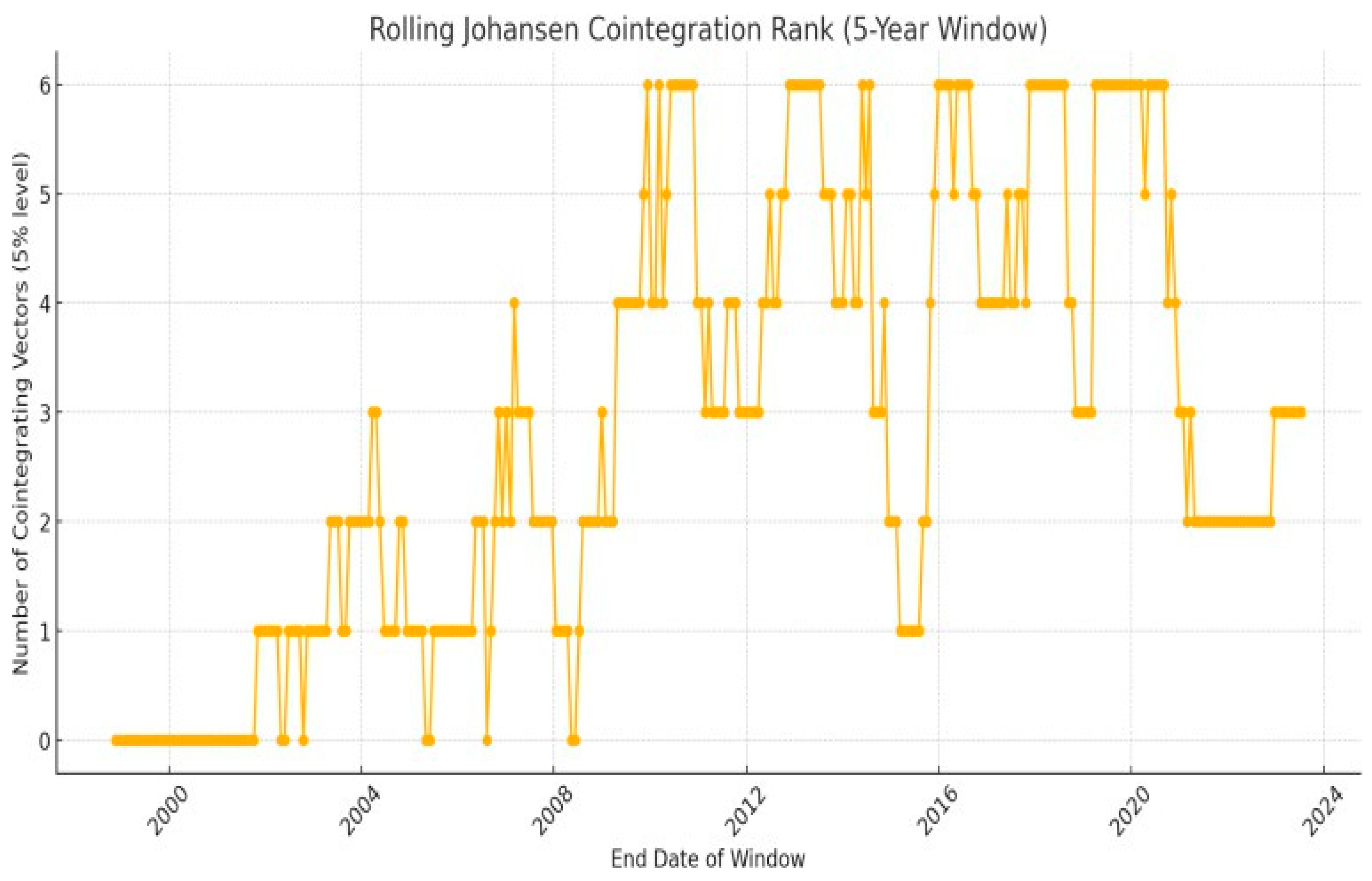
Table 1.
Market Capitalisation (M-Cap) of Selected Countries.
| Country | M-Cap (2024) | Share in World M-Cap | Rank |
| USA | 49 Mil. US$ | 44.74% | 1 |
| China | 10 Mil. US$ | 9.12% | 2 |
| Japan | 5 Mil. US$ | 5.64% | 3 |
| India | 4 Mil. US$ | 4.50% | 4 |
| U.K. | 2 Mil. US$ | 2.77% | 7 |
Source: Author’s Calculations based on approximate figures.
Table 2.
Descriptive Statistics.
| Pre-COVID period | Post-COVID period | |||||||||||
| Particulars | India | China | Hong Kong | Japan | UK | US | India | China | Hong Kong | Japan | UK | US |
| Average Return | 0.066 | 0.017 | 0.023 | 0.02 | 0.094 | 0.027 | 0.05 | 0.01 | -0.05 | 0.02 | -0.01 | 0.03 |
| Maximum Return | 0.15 | 0.09 | 0.16 | 0.13 | 0.11 | 0.1 | 0.08 | 0.07 | 0.08 | 0.07 | 0.08 | 0.08 |
| Minimum Return | -0.12 | -0.12 | -0.14 | -0.12 | -0.1 | -0.13 | -0.08 | -0.08 | -0.05 | -0.06 | -0.11 | -0.12 |
| Standard Deviation | 1.51 | 1.73 | 1.54 | 1.59 | 1.25 | 1.26 | 0.016 | 0.012 | 0.016 | 0.015 | 0.015 | 0.017 |
Table 5.
Results of Unit Root Test.
| Pre-COVID Period | Post-COVID Period | |||||||
| Original Level | First Differencing | Original level | First differencing | |||||
| Particulars | T-stats | Prob | t-Stats | Prob | T-stats | Prob | T-stats | Prob |
| India | 0.25 | 0.9 | -59.9 | 0.01 | -0.86 | 0.7 | -22.6 | 0 |
| China | -1.83 | 0.36 | -61.4 | 0.01 | -1.97 | 0.29 | -21.15 | 0 |
| Hong Kong | -1.71 | 0.42 | -62.5 | 0.01 | -1.65 | 0.45 | -21.4 | 0 |
| Japan | -0.76 | 0.82 | -62.1 | 0.01 | -1.41 | 0.57 | -14.15 | 0 |
| UK | -1.62 | 0.47 | -62.1 | 0.01 | -1.95 | 0.3 | -23.44 | 0 |
| US | 0.99 | 0.99 | -63.8 | 0.01 | -1.36 | 0.59 | -14.38 | 0 |
(Source: author’s calculation).
Table 6.
Results of Johansen Co-integration.
| Pre-COVID Period | Post COVID Period | |||
| Hypothesized number of Co-integrated Equation(s) | Trace Statistic | Max-Eigen Statistic | Trace Statistic | Max-Eigen Statistic |
| None* | 95.92* | 0.008* | 98.18* | 35.37 |
| At most 1 | 65.64 | 0.006 | 62.8 | 29.44 |
| At most 2 | 41.08 | 0.005 | 33.35 | 13.05 |
| At most 3 | 20.58 | 0.002 | 20.3 | 10.72 |
| At most 4 | 9.68 | 0.002 | 9.573 | 5.04 |
| At most 5 | 1.62 | 0.004 | 4.52* | 4.52* |
(Source: author’s calculation).
Table 6. 1.
Robustness Check: Post-COVID Johansen Co-integration Analysis.
| Hypothesized number of Co-integrated Equation(s) | Trace Statistic | Max-Eigen Statistic |
| None* | 212.15 | 82.95 |
| At most 1* | 129.20 | 47.61 |
| At most 2* | 81.59 | 39.15 |
|
At most 3* |
42.44 |
30.06 |
| At most 4 | 12.37 | 10.43 |
(Source: author’s calculation).
Table 7.
Results of Granger Causality.
| Pre-COVID Period | Post-COVID Period | |||||||
| Null Hypothesis: No Causality from Country X to Country Y (X ↛ Y) | Chi-square Statistics | Prob | Result | Causality | Chi-square Statistics | Prob | Result | Causality |
| China ↛ India | 7.75 | 0.1 | Accepted | Uni-directional | 7.17 | 0.02 | Rejected | Uni-directional |
| India ↛ China | 9.64 | 0.04 | Rejected | 0.79 | 0.6 | Rejected | ||
| Hong Kong ↛ India | 9 | 0.06 | Accepted | Uni-directional | 2.5 | 0.28 | Accepted | No Casuality |
| India ↛ Hong Kong | 12.49 | 0.01 | Rejected | 5.21 | 0.07 | Accepted | ||
| Japan ↛ India | 14.89 | 0 | Rejected | Bi-Directional | 1.38 | 0.49 | Accepted | Uni-directional |
| India ↛ Japan | 10.79 | 0.02 | Rejected | 8.35 | 0.01 | Rejected | ||
| UK ↛ India | 5.72 | 0.22 | Accepted | Uni-directional | 3.79 | 0.15 | Accepted | Uni-directional |
| India ↛ UK | 20.28 | 0 | Rejected | 12.05 | 0 | Rejected | ||
| USA ↛ India | 153.18 | 0 | Rejected | Bi-Directional | 18.1 | 0 | Accepted | Bi-Directional |
| India ↛ USA | 12.33 | 0.01 | Rejected | 5.99 | 0.04 | Rejected | ||
(Source: author’s calculation).
Table 8.
Descriptive statistics.
| Pre-global Crises | Post-Global crises | |||||||||||
| Particulars | India | China | Hong Kong | Japan | UK | US | India | China | Hong Kong | Japan | UK | US |
| Average Return | 0.014 | 0.089 | 0.072 | 0.029 | 0.014 | 0.018 | 0.003 | -0.001 | -0.0005 | 0.017 | 0.005 | 0.031 |
| Maximum Return | 0.07 | 0.08 | 0.05 | 0.06 | 0.06 | 0.05 | 0.15 | 0.09 | 0.16 | 0.13 | 0.11 | 0.1 |
| Minimum Return | -0.11 | -0.09 | -0.06 | -0.09 | -0.05 | -0.04 | -0.12 | -0.12 | -0.14 | -0.12 | -0.11 | -0.13 |
| Standard Deviation | 0.015 | 0.016 | 0.012 | 0.014 | 0.011 | 0.01 | 0.011 | 0.016 | 0.016 | 0.016 | 0.013 | 0.014 |
(Source: author’s calculation).
Table 9.
Jarque-Bera Test.
| Pre-global Crises | Post-global crises | |||||||||||
| Particulars | India | China | Hong Kong | Japan | UK | US | India | China | Hong Kong | Japan | UK | US |
| Skewness | -0.53 | -0.01 | -0.05 | -0.3 | -0.11 | 0.07 | -0.13 | -0.51 | 0.17 | -0.63 | -0.3 | -0.73 |
| Kurtosis | 8.4 | 6.7 | 5.85 | 6.3 | 7.5 | 5.89 | 15.21 | 8.64 | 15.77 | 11.64 | 14.01 | 16.9 |
| Test Stats | 1561.9 | 706.3 | 419.2 | 582.6 | 1046.3 | 433.3 | 18754.9 | 4138.37 | 20519.4 | 9585.11 | 15281.6 | 24557.6 |
| Probability | 0 | 0 | 0 | 0 | 0 | 0 | 0 | 0 | 0 | 0 | 0 | 0 |
(Source: author’s calculation).
Table 10.
Correlation matrix.
| Pre-global Crises | Post-global Crises | |||||||||||
| Country | India | China | Hong Kong | Japan | UK | US | India | China | Hong Kong | Japan | UK | US |
| India | 1 | 0.74 | 0.97 | 0.92 | 0.91 | 0.93 | 1 | 0.44 | 0.62 | 0.94 | 0.72 | 0.98 |
| China | 1 | 0.81 | 0.56 | 0.6 | 0.64 | 1 | 0.51 | 0.52 | 0.34 | 0.42 | ||
| Hong Kong | 1 | 0.85 | 0.88 | 0.92 | 1 | 0.7 | 0.79 | 0.61 | ||||
| Japan | 1 | 0.95 | 0.92 | 1 | 0.77 | 0.95 | ||||||
| UK | 1 | 0.95 | 1 | 0.72 | ||||||||
| USA | 1 | 1 | ||||||||||
(Source: author’s calculation).
Table 11.
Results of Unit root test.
| Pre-Global Crises | Post-global crises | |||||||
| Original Level | First differencing | Original level | First Differencing | |||||
| Particulars | T-stats | Prob | T-Stats | Prob | T-stats | Prob | T-stats | Prob |
| India | 1.92 | 0.99 | -33.6 | 0 | 0.26 | 0.75 | -54.6 | 0 |
| China | 0.53 | 0.98 | -7.11 | 0 | -3.47 | 0.23 | -48.8 | 0 |
| Hong Kong | 1.96 | 0.99 | -18.35 | 0 | -2.52 | 0.11 | -49.8 | 0 |
| Japan | -0.88 | 0.79 | -35.36 | 0 | -0.91 | 0.78 | -33.9 | 0 |
| UK | -0.42 | 0.89 | -38.43 | 0 | -2.71 | 0.07 | -50.4 | 0 |
| US | -0.53 | 0.88 | -37.55 | 0 | -0.46 | 0.89 | -24.8 | 0 |
(Source: author’s calculation).
Table 12.
Results of Johansen Co-integration.
| Pre-Global crises | Post-Global crises | |||
| Hypothesized number of Co-integrated Equation(s) | Trace Statistic | Max-Eigen Statistic | Trace Statistic | Max-Eigen Statistic |
| None* | 116.6* | 47.7* | 98.0* | 0.016* |
| At Most 1 | 69.23 | 31.8 | 56.2 | 0.008 |
| At Most 2 | 37.41 | 16.09 | 33.8 | 0.006 |
| At Most 3 | 21.32 | 12.09 | 18.2 | 0.003 |
| At Most 4 | 9.22 | 5.19 | 8.16 | 0.002 |
| At Most 5 | 4.03* | 4.03* | 1.07 | 0.004 |
*At the 5% significance level, the hypothesis was rejected. (Source: author’s calculation)
Table 13.
Results of Granger Causality Test.
| Pre-Global crises | Post-Global crises | |||||||
| Null Hypothesis: No Causality from Country X to Country Y (X ↛ Y) | Chi-square Statistics | Probability | Result | Causality | Chi-square Statistics | Probability | Result | Causality |
| China ↛ India | 13.12 | 0.06 | Accepted | Uni-directional | 8.68 | 0.01 | Rejected | Uni-directional |
| India ↛ China | 14.4 | 0.04 | Rejected | 3.17 | 0.2 | Accepted | ||
| Hong Kong ↛ India | 49.4 | 0 | Rejected | Bi-directional | 2.43 | 0.2 | Accepted | Uni-directional |
| India ↛ Hong Kong | 18.8 | 0 | Rejected | 29.19 | 0 | Rejected | ||
| Japan ↛ India | 8.84 | 0.26 | Accepted | No causality | 3.29 | 0.1 | Accepted | Uni-directional |
| India ↛ Japan | 7.11 | 0.41 | Accepted | 12.2 | 0 | Rejected | ||
| UK ↛ India | 21.98 | 0 | Rejected | Uni-directional | 4.34 | 0.1 | Accepted | Uni-directional |
| India ↛ UK | 2.94 | 0.89 | Accepted | 23.5 | 0 | Rejected | ||
| USA ↛ India | 146.35 | 0 | Rejected | Uni-directional | 88.1 | 0 | Rejected | Bi-directional |
| India ↛ USA | 13.17 | 0.06 | Accepted | 16.6 | 0 | Rejected | ||
(Source: author’s calculation).
Table 13. 1.
Granger Causality Results (India–US) across 2002–2007, 2008–2009 and 2010–2019
| Pre-Global crises | Global Crises | Recovery Period | ||||||||||
| Null Hypothesis: Y (X ↛ Y) | Chi-Square Stats | P-value | Result | Causality | Chi-Square Stats | P-value | Result | Causality | Chi-Square Stats | P-value | Result | Causality |
| USA ↛ India | 6.00 | 0.00 | Rejected | Uni-directional | 0.52 | 0.06 | Accepted | No-Causality | 12.35 | 0.00 | Rejected | Uni-directional |
| India ↛ USA | 2.45 | 0.09 | Accepted | No-causality | 0.12 | 0.2 | Accepted | No-Causality | 2.65 | 0.10 | Accepted | No-causality |
Source: Author’s Calculation.
Disclaimer/Publisher’s Note: The statements, opinions and data contained in all publications are solely those of the individual author(s) and contributor(s) and not of MDPI and/or the editor(s). MDPI and/or the editor(s) disclaim responsibility for any injury to people or property resulting from any ideas, methods, instructions or products referred to in the content. |
© 2025 by the authors. Licensee MDPI, Basel, Switzerland. This article is an open access article distributed under the terms and conditions of the Creative Commons Attribution (CC BY) license (http://creativecommons.org/licenses/by/4.0/).
Copyright: This open access article is published under a Creative Commons CC BY 4.0 license, which permit the free download, distribution, and reuse, provided that the author and preprint are cited in any reuse.


