
Submitted:
25 November 2025
Posted:
28 November 2025
You are already at the latest version
Abstract
Estimating the mass of Oudemansiella raphanipies quickly and accurately is indispensable for optimizing post-harvest packaging processes. The traditional methods typically involve manual grading followed by weighing with a balance, which is inefficient and labor-intensive. To address the challenges encountered in actual production scenarios, in this work, we proposed a novel pipeline for estimating the mass of multiple Oudemansiella raphanipies. To achieve this goal, an enhanced deep learning (DL) algorithm for instance segmentation and a machine learning (ML) model for mass prediction were introduced. On one hand, to segment the multiple samples in the same image, a novel instance segmentation network named FinePoint-ORSeg was presented to obtain the finer edges of samples, which integrated the edge attention module for improving the fineness of the edges. On the other hand, for individual samples, a novel cap-stem segmentation approach was applied and 18 phenotypic parameters were obtained. Furthermore, the Principal Component Analysis (PCA) was utilized to reduce the redundancy among features. Combining the two aspects mentioned above, the mass was computed by Exponential GPR model with 7 principal components. In terms of segmentation performance, our model outperforms the original Mask R-CNN, the AP, the AP50, the AP75 and the APs are improved by 2%, 0.7%, 1.9%, and 0.3%, respectively. Additionally, our model outperforms other networks such as YOLACT, SOLOV2 and Mask R-CNN with swin. As for mass estimation, the results showed the average Coefficient of Variation (CV) of single sample mass in different attitude are 6.81%. Moreover, an average mean absolute percentage error (MAPE) of multiple samples is 8.53%. Overall, the experimental results indicated that the proposed method is time-saving, non-destructive and accurate. This can provide a reference for the research on post-harvest packaging technology of Oudemansiella raphanipies.
Keywords:
edible mushroom
; machine learning
; mass estimation
; mushroom phenotype
1. Introduction
Oudemansiella raphanipies is a precious edible mushroom, which not only contains essential nutrients such as protein, fat, amino acids, and various vitamins, but also contains a certain amount of polyphenols and polysaccharides [1]. Additionally, its unique flavor, rich nutritional value, and excellent antioxidant activity make it increasingly popular among consumers. Thus, Oudemansiella raphanipies has gained popularity as a cultivated crop among mushroom farmers. However, the surge in Oudemansiella raphanipies production has intensified post-harvest packaging and processing difficulties, attributable to its high water content and absence of epidermal tissue. Post-harvest delays in packaging and storage accelerate the quality loss in mushrooms, adversely impacting their marketability and farmer income. This is also one of the key factors hindering the rapid development of the Oudemansiella raphanipies industry.
Typically, the packaging of post-harvest agricultural products is based on mass. To improve weighing efficiency, electronic weighing equipment is used to replace traditional mechanical weighing devices [2]. However, during the operation process, workers may cause physical damage, which further reduce the value of samples. With the rapid development of computer vision technology, non-destructive mass estimation has emerged as the predominant methodology. One method is to determine the mass of the sample by measuring its volume. This approach relies on the principle that the density of a homogeneous material is constant, implying a direct proportional relationship between volume and mass. Currently, researchers have achieved satisfactory accuracy in the volume measurement of many agricultural products such as watermelon [3], apple [4], egg [5,6], orange [7], cucumber and carrot [8]. Another method is to estimate the mass of samples by regression method based on phenotypic parameter. Similarly, many researchers have successfully developed regression models to estimate the mass of agricultural products, such as apple [9], kiwi fruit [10], tomato [11] and potato [12]. In contrast to other agricultural products, Oudemansiella raphanipies is not symmetrical and there are undetermined hollowed-out areas at the bottom when they are processed on the conveyor belt. Therefore, it is difficult to measure the volume of Oudemansiella raphanipies directly by image-based method, thus the approach of estimating mass by volume is not work. From another perspective, owing to the distinct morphological characteristics of Oudemansiella raphanipies compared to conventional agricultural commodities, regression models relying exclusively on basic phenotypic parameters (e.g., length and width) exhibit substantial errors in mass estimation. Furthermore, Oudemansiella raphanipies commonly handled in batches rather than processed individually in practical production due to the small size of individual unit. Consequently, it is necessary to design a new means to obtain the mass of a batch of Oudemansiella raphanipies in rapidly and accurately way. For this purpose, the task can be divided to three subtasks, including segmentation of multiple samples, extract multiple complex phenotypic parameters and select appropriate parameters and approaches for mass regression.
For separating samples, it belongs to the instance segmentation task in the field of computer vision. With the development of computer hardware and deep learning, various instance segmentation networks have emerged rapidly, such as Mask R-CNN [13], YOLACT [14], SOLOV2 [15] and Mask R-CNN with swin [16]. These approaches have achieved impressive performance on agriculture field. For instance, Yang et al. [17] and Li et al. [18] applied the Mask R-CNN to segment the soybean to calculate the phenotypic parameters and the experiment results showed that the method is robust for segmenting the targets even under densely-cluttered environment. Sapkota et al. [19] compared the YOLOv8 and Mask R-CNN with immature green fruit and trunk and branch datasets. The experimental results showed that both of them effectively segmented apple tree canopy images from both dormant and early growing seasons, and YOLOv8 showed slightly better performance in different environments. Moreover, to solve the problem that the rice field detection technology cannot adapt to the complexity of the real-world, Chen et al. [20] considered the rice row detection problem as an instance segmentation problem and successfully implemented a two-pathway-based method. However, the application of these advanced methods in the field of edible mushroom is scarce, especially for Oudemansiella raphanipies.
For phenotypic parameters subtask, recent advances in computer vision and deep learning techniques have powered research in and application of automatic phenotype extraction in agronomy. Yang et al. [17] applied principal component analysis (PCA) to correct the pod’s direction and then calculate the width and length of pod length with the revised bounding box of corrected pod. The results showed that the average measurement error for pod length was 1.33 mm, with an average relative error of 2.90%, while the pod width had an average measurement error of 1.19 mm and the average relative error of 13.32%. Except for length and width, He et al. [21] extracted pod's area using the minimum circumscribed rectangle method combined with the template calibration method and the results showed that the accuracy of pod area was 97.1%. Additionally, Liu et al. [22] proposed a core diameter Ostu method to judge the posture and then obtained the length, surface area and volume, which calculated by elliptic long and short axis of the cross section of silique. The experimental results reported that the errors of all phenotypic parameters were less than 5.0%. To meet the phenotypic information requirements of Flammulina filiformis breeding, Zhu et al. [23] utilized image recognition technology and deep learning models to automatically calculate phenotypic parameters of Flammulina filiformis fruiting bodies, including cap shape, area, growth position, color, stem length, width, and color. Furthermore, some studies apply the extracted phenotypic characteristics to other tasks. Kumar et al. [24] extracted the centroid, main axis length, and perimeter of plant leaves and then combined them with multiple classifiers to achieve classification. The accuracy of this method can reach 95.42%. Moreover, Okinda et al. [25] fitted the egg to an ellipse using Direct Least Square method and then extracted 2D features of the ellipse, such as area, eccentricity and perimeter, to establish the relationship between these parameters and the product's volume using thirteen regression models, achieving excellent results in volume estimation of the egg. However, despite the previous studies have obtained the basic parameters of Oudemansiella raphanipies like length and width [26,27], these characteristics cannot fully represent the morphology of Oudemansiella raphanipies. Thus, to obtain an accurate mass result, more complex phenotypic parameters of Oudemansiella raphanipies need to be calculated.
For mass estimation subtask, existing research has primarily focused on mathematical models-based method and regression-based method. Due to the irregularity of agricultural products, in practice scene, more and more regression-based methods are being used. For instance, Nyalala et al. [28] directly feed five phenotypic parameters of tomato (area, perimeter, eccentricity, axis-length, and radial distance) into Support Vector Machine (SVM) with different kernels and Artificial Neural Network (ANN) with different training algorithms models to predict its mass. Experimental results showed that the Bayesian regularization ANN outperformed other models, with a root mean square error (RMSE) of 1.468g. Nevertheless, this approach neglected feature redundancy and correlations between predictors and target variables. To make up this insufficiency, Saikumar et al. [29] calculated a high linear correlation between the mass and the length, width, perimeter, and projection area first with a correlation coefficient of 0.96, 0.92, 0.92 and 0.95, respectively, and built multiple univariate and multivariate regression models for elephant apple (Dillenia indica L.) mass prediction. The results showed that the multivariate rational model performed the best, with a RMSE of 18.196g. However, this simplistic variation of input combinations did not consider potential redundancy among the input parameters, which could lead to suboptimal model performance. Moreover, the performance of regression models varies depending on the target object. Consequently, to accurately predict the mass of Oudemansiella raphanipies, it is essential to explore optimal model selection and feature optimization strategies.
In this study we implemented a machine learning and deep learning-based framework for estimating the mass of a batch of Oudemansiella raphanipies. The main contributions are:
1) A dataset includes 1201 images was constructed and a novel instance segmentation network for Oudemansiella raphanipes Segmentation (FinePoint-ORSeg) was applied to obtain the individual sample;
2) A novel stem-cap-based segmentation method is proposed for extracting phenotypic parameter robustly, and 18 phenotypic parameters were extracted;
3) Evaluate the performance of various mass regression methods and the best means for calculating mass of multiple Oudemansiella raphanipies was determined.
2. Materials and methods
2.1. Materials
2.1.1. Image Acquisition System
The image acquisition system consists of a camera (RealSense SR305, Intel, California, America), a computer (Intel Core i5-7500, 16GB memory), two LED light and a camera holder as shown in Figure 1. Since the proposed method will be applied to the postharvest packaging assembly line of Oudemansiella raphanipies, the imaging background is set to green to consistent with conveyor belt. The distance between the camera and the Oudemansiella raphanipies was maintained at 31.5 cm to ensure a sufficient number of samples in field of view. The RGB image is transferred to the computer via a USB 3.0 data cable and saved in the "PNG" format (640 × 480 pixels).
2.1.2. Dataset
The samples in our work were collected from the School of Biological Science and Engineering, Jiangxi Agricultural University in May 2024 and the edible mushroom factory in Zhangshu City, Jiangxi Province from January to November 2024. Four sub-datasets (Dateset1, Dateset2, Dateset3, Dateset4) were established for our work as shown in Figure 2.
Dataset 1 totally contains 1201 labeled images and each image contains several (1-10) Oudemansiella raphanipes. Dataset 2 is used to build the mass regression model, where each sample is shoot from different angles 7 times at the image center. After removing the blurry images, a total of 1475 images remain. Additionally, we randomly split the Dataset 1 and 2 into a training set and a validation set in an 8:2 ratio, respectively.
On the assembly line, it is easy to fix a camera above the conveyor belt and clearer images can be obtained by controlling the conveyor speed. However, the states of the Oudemansiella raphanipes in the images cannot be determined. Therefore, we additionally set up two datasets, Dataset 3 and Dataset 4 to validate the model's performance. To explore the robustness of the mass estimation model under different placement states of Oudemansiella raphanipes, Dataset 3 includes 24 Oudemansiella raphanipes and a total of 240 images, where each sample was randomly thrown 10 times respectively. Dataset 4 contains 30 Oudemansiella raphanipes images, with 10 large (L) samples, 10 medium (M) samples, and 10 small (S) samples, which classified by experienced farmers and partial examples are shown in Figure 3. Meanwhile, for each sample, we manually measured the cap diameter and height, as well as the stem diameter and height, as shown in Table 1. For each grade, 10 Oudemansiella raphanipes are grouped together and then randomly thrown on the platform 10 times. This Dataset can be used to evaluate the accuracy of the proposed pipeline for the mass of multiple Oudemansiella raphanipes. Additionally, high-precision densitometer (MDJ-300S, LICHEN technology, Shanghai, Chian) was applied to acquire the ground truth of mass and volume of dataset 2, 3 and 4.
2.2. Methods
The main objective of this study is to predict the mass of multiply Oudemansiella raphanipes. To achieve this goal, the pipeline is described as follow: First, an instance segmentation network is trained to segment individual samples, with the specific steps shown in the Oudemansiella raphanipes instance segmentation Figure 4 (a). Then, based on the Oudemansiella raphanipes mask, a shape prior-based cap-stem segmentation algorithm is presented for building a mass regression model Figure 4 (b). Finally, combining the results of above step, the mass of Oudemansiella raphanipes is obtained Figure 4 (c). Since the volume of a solid is closely related to its mass, we also conducted a regression analysis on the volume.
2.2.1. FinePoint-ORSeg Model for Sample Segmentation
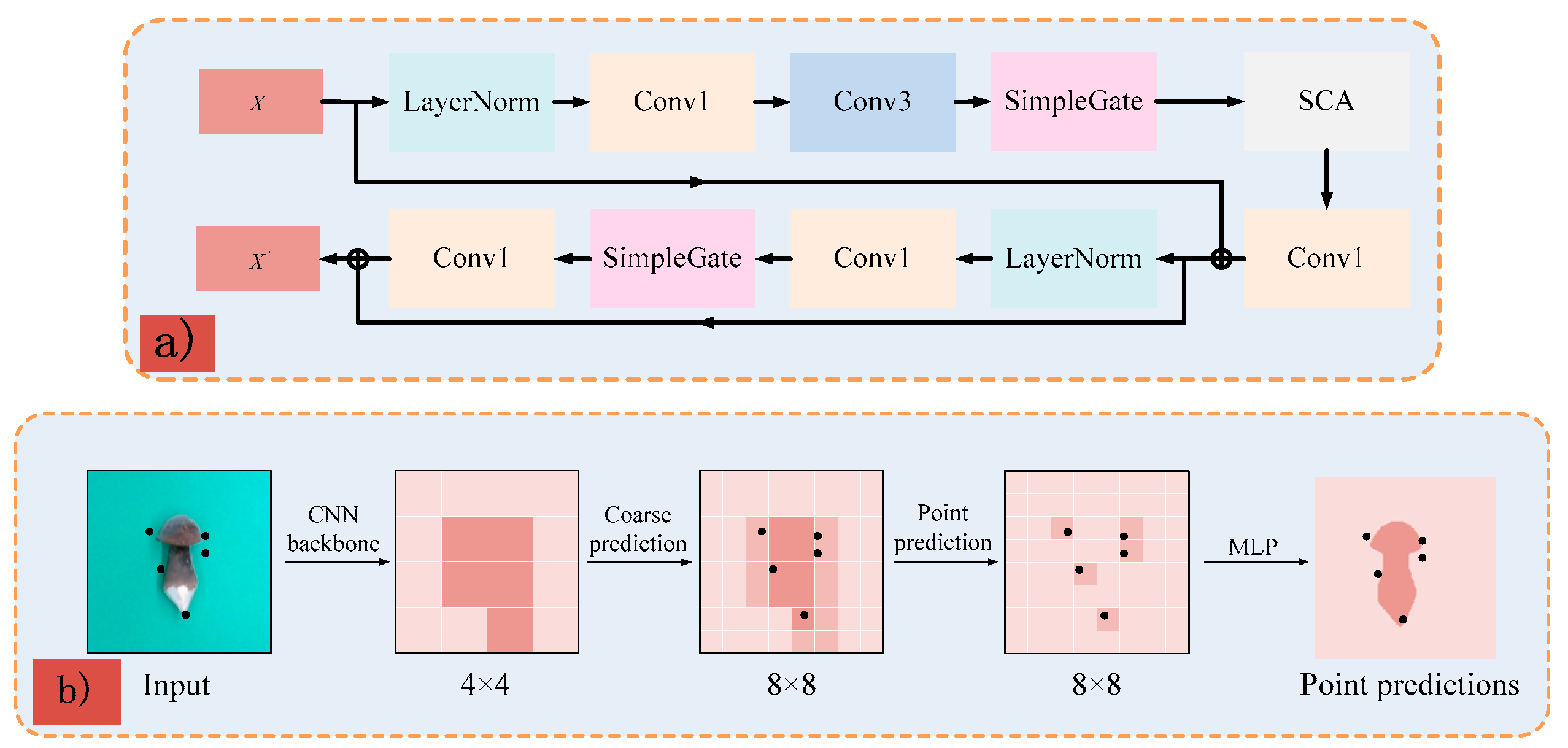
Mask R-CNN [13] is a classical deep learning model specifically designed for instance segmentation tasks. As a method based on Convolutional Neural Networks (CNNs), Mask R-CNN relies on convolutional layers to extract features during the segmentation process. However, convolution operations have the characteristic of a local receptive field, which may lead to blurring effects when processing image details, especially at the edges, resulting in less smooth or precise boundaries. For general applications, such as animal or vehicle segmentation, this doesn't have adverse effect on the results. Nevertheless, in our task, it may result in inaccurate phenotypic parameters. Therefore, we hope to obtain finer edge shapes by introducing PointRend module [30]. Additionally, considering that traditional nonlinear activation functions (such as ReLU, Sigmoid/Tanh) have significant drawbacks in information transmission, which severely damage high-frequency details of the image (such as sharp edges) and result in information loss or distortion, causing blurred results, inaccurate boundaries, and loss of details. Therefore, we have also embedded the NAF block [31] to improve the model's performance. The structures of above two modules are shown in Figure 5.
(1) PointRend module
PointRend (Point-based Rendering) is an image segmentation refinement module based on adaptive point sampling. Its core goal is to improve the segmentation accuracy of object boundaries and detailed regions through an iterative refinement strategy, which can precisely provide us with more accurate segmentation results for the subsequent extraction of phenotypic parameters. The workflow of this module can be divided into three key stages module as shown in Figure 6 (a). First, PointRend module uses a mixed strategy of uncertainty sampling and uniform sampling to select a set of candidate points for refinement from the initial coarse-grained segmentation results. For each candidate point, the module extracts corresponding feature vectors from different layers of the backbone network and aligns them to the target point's spatial coordinates using bilinear interpolation. Then, feature concatenation is performed to merge low-level high-resolution detail information with high-level semantic information, forming a point-level feature vector with rich contextual representation. The fused feature vector is then passed through a small multi-layer perceptron (MLP) to predict the refined segmentation result for each point. The MLP is designed for efficient computation, and its output is the binary classification probability (foreground / background) for each candidate point. Finally, the refined point predictions are interpolated back to the original resolution and merged with the coarse segmentation map to generate a high-precision segmentation mask.
(2) Nonlinear Activation Free block
Traditional activation functions (such as ReLU) introduce information truncation in nonlinear transformations (e.g., ReLU sets negative values to zero), which may lead to the loss of feature details. In contrast, segmentation tasks rely on pixel-level localization, and NAF may preserve more high-frequency details (such as object edges), improving the boundary accuracy of the mask. As shown in Figure 6 (b) is the structure of the Nonlinear Activation Free block (NAF) block. Given a feature map X, the gated linear units can be calculated as Eq. (1):
Where the and are linear transformers, is a no-linear activation function, and the represents element-wise multiplication. However, this operation may increase the intra-block complexity, thus the authors revisit the activation function as Eq. (2):
Where the Φ refers to the cumulative distribution function of the standard normal. Furthermore, comparing Eq. (1) and Eq. (2), it can be observed that due to the inherent nonlinearity of the GLU function, the formula still holds even when σ is removed. Therefore, directly splitting the feature map into two parts along the channel dimension and multiplying them can reduce complexity as shown in Eq. (3):
Where Y is a feature map of the same size as X.
Additionally, the authors compress spatial information into channel information and utilize a multi-layer perceptron to attend to the channels to capture global information, as demonstrated by the calculation in Eq. (4):
Where W1 and W2 are fully-connected layers and ReLU is adopted between two fully-connected layers, * is a channelwise product operation. Further, if we consider the channel-attention calculation as a function noted as Ψ, then the Eq. (4) can be rewritten as Eq. (5):
Compared with the Eq. (5) with Eq. (2), we find that the two are similar. This inspires us to explore whether we can simplify Eq. (5) in a similar manner to Eq. (2), by aggregating global information and channel information to retain channel attention. Thus, the Simplified Channel Attention can be represented as Eq. (6):
Figure 6.
(a) Example of how the PointRend module works. (b) The structure of NAF block.
2.2.2. Shape Prior-Based Phenotypic Extraction Algorithm
(1) Cap-stem segmentation algorithm
Since the Oudemansiella raphanipies consists of the cap and stem, it is necessary to segment the stem and cap for the convenience of subsequent phenotypic parameter measurements. Based on the morphological characteristics of the Oudemansiella raphanipies, a novel cap-stem segmentation algorithm was presented in Figure 7, the detail procedure includes the following steps:
(a) Extract ordering contour point. In phenotype parameters obtaining task, a key step is to calculate the position of the measurement point. Despite the function find_contours in OpenCV library can obtain sorted contours, however they are discontinuous, which may filter out the position we need. Thus, a new contour sorting approach needs to be developed. Establish an image coordinate system with the top-left corner as the origin. Traverse the image G_(x, y) from top to bottom, left to right, if the pixel value G_(x, y) at the current position is 255, and there exists at least one neighboring pixel with a value of 0 in the 8-connected neighborhood, the current pixel is considered a contour point; Otherwise, it is considered an interior point, as shown in Eq. (7).
With the contour point , random select a contour point from as the starting point of the ordered contour. As shown in Eq. (8), calculate the Euclidean distance between point and other points , which the points in but not in . Then add the point with the shortest distance as the next point in the ordered contour. Then, calculate the Euclidean distance between point and the remaining points , which the points in but not in , and again add the point with the shortest distance as the next point in the ordered contour which the points in but not in . Repeat above process until all contour points have been traversed and obtain the compete ordered contour .
(b) Extract the segmentation points. After obtaining the ordering contour points , calculate the vectors (Eq. 9) from the current point to the previous m points, and the vectors (Eq. 10) from the current point to the next m points. Then, compute the angle between vectors and , if angle is smaller than the threshold , the current point is considered as a segmentation point (Eq. 11). Based on multiple experiments and the morphological structure of Oudemansiella raphanipies, the value of m was chosen to be 7 and the was set to 135 degrees.
(c) Filter segmentation points. Due to the morphological variations of Oudemansiella raphanipies, neighboring positions around the segmentation points may also meet the threshold set by Eq. (12). Therefore, it is necessary to filter the obtained segmentation points and select two points as the final segmentation points. With the segmentation points , random select a segmentation point from as the starting point of the filtered segmentation points. Calculate the Euclidean distance between the current point and the other unfiltered points of . If the distance is smaller than the threshold, remove this unfiltered point from and recompute the distance to the next unfiltered point of . Repeat the calculation until find a point that the distance greater than the threshold, and consider this point as another segmentation point . Thus, the points and were considered as the final segmentation points.
Where the refer to the points of the unfiltered segmentation points besides and , and the was set to 10.
(d) Obtained the cap and stem region. After obtaining the segmentation points of the stem and cap , divide the ordered contour into two contours, and . Then, calculate the centroid (Mx, My) of the ordered contour obtained in Step 1. If (Mx, My) lies within the range of , then is the stem region and is the cap region; if (Mx, My) lies within the range of , then is the stem region and is the cap region.
(2) Definition of phenotypic parameters
By cap-stem segmentation algorithm, the separate masks of cap and stem can be obtained. However, the randomly placed sample may cause the Oudemansiella raphanipies to be tilted, making it hard to directly measurement the parameters by bounding box, and would introduce systematic error, as shown in Figure 8 (a). To overcome this drawback, we first used the principal component analysis (PCA) algorithm to acquire the main direction of the cap (stem) as shown in Figure 8 (b). Then, we rotated the cap (stem) so that the main direction aligned with the image coordinate system, as shown in Figure 8 (c). Figure 8 (d) illustrates the five primary phenotypic parameters (CD, CH, Angle, SH, SD,), and 18 phenotypic parameters is defined in Table 1.

Table 1.
Definition of 18 Phenotypic parameters.
| ID | Phenotypic parameters |
Equations | Units |
| 1 | CD | mm | |
| 2 | SD | mm | |
| 3 | CH | mm | |
| 4 | SH | mm | |
| 5 | - | ||
| 6 | - | ||
| 7 | mm | ||
| 8 | mm | ||
| 9 | |||
| 10 | |||
| 11 | - | ||
| 12 | - | ||
| 13 | - | ||
| 14 | - | ||
| 15 | - | ||
| 16 | mm | ||
| 17 | mm | ||
| 18 | |||
| Note: the coordinate () represented the cap (stem / fruit body) mask; the was the area of the convex hull of the cap (stem) mask. | |||
2.2.3. Mass Estimation Model
To predict the mass of an Oudemansiella raphanipies based on phenotypic parameters, nine regression models were evaluated in this study (Table 2): Support Vector Machine (SVM) (Linear, Fine Gaussian, Medium Gaussian and Coarse Gaussian), Gaussian Process Regression (GPR) (Rational Quadratic and Exponential) and Artificial Neural Networks (ANN) (Bayesian Regularization, Levenberg-Marquardt, and Scaled Conjugate Gradient training algorithms).
Support Vector Machine (SVM) [32] is a powerful supervised learning algorithm primarily used for classification and regression tasks. Further, SVM can be extended into Support Vector Regression (SVR), a regression method that can utilize multiple different kernel functions such as Linear and Gaussian kernel to solve nonlinear problems. For example, Nyalala et al. [33] used SVM with different kernels to predict the volume and mass of tomatoes, and the accuracy were all above 90%.
Gaussian Process Regression (GPR) [34] is a non-parametric regression method based on Bayesian inference, using Gaussian processes (GP) as the prior model for the target function. Similar to SVM, different types of data require distinct kernel functions to characterize their underlying structure. Consequently, selecting appropriate kernel functions is critical for enhancing both the performance and flexibility of Gaussian Process Regression (GPR) models. Okinda et al. [25] used the Exponential Gaussian Process to predict the volume of a single egg, achieving an excellent result with an RMSE of 1.175 cm3 and R2 of 0.984. Moreover, Gonzalez et al. [35] estimated the weight of rice based on Exponential kernel and rational quadratic GPR, which obtained a RMSE of 31.081 g and 31.115 g, respectively. This study will explore the performance of two kernel functions, Rational Quadratic and Exponential, in estimating the mass and volume of Oudemansiella raphanipies.
Compared with the SVM and GPR methods, the advantage of Artificial Neural Networks (ANN) [36] lies in the fact that there is no need to manually design the kernel function and they can automatically capture complex deep structures. During the learning process, the network's objective is to adjust parameters using optimization algorithms to minimize prediction errors. Depending on the different optimization algorithms, the commonly used ANN networks include Bayesian Regularization, Levenberg-Marquardt, and Scaled Conjugate Gradient ANN [37] and they have all been well applied in different scenarios. Kayabaşı et al. [38] obtained 5 features (length, width, area, perimeter and fullness) of wheat and then applied the Bayesian Regularization ANN to identify the grain type of wheat. Amraei et al. [39] predicted broiler mass based on different ANN techniques, while Bayesian Regulation ANN was the best network with R^2 value of 0.98. Sofwan et al. [36] utilized the Levenberg-Marquardt ANN to predict the air temperature inside of the greenhouse 30 minutes in the future, which helps adjust the growing environment of the Water spinach.
2.2.4. Implementation Details
All DL and ML algorithms were run on the Ubuntu 20.04.6 (GNU/Linux 5.14.0-1051-oem x86_64) operating system (Intel(R) Xeon(R) Silver 4112 CPU @ 2.60GHz, 64 GB of RAM and NVIDIA GeForce RTX 5000 GPUs), using the PyTorch 1.7.1 framework and Python 3.7. The CUDA version 11.7 was used for this experiment. The software used to train the model was PyCharm 2019.
To fine-tune the dataset of DL model during the training process, we used the pretraining weight trained on the open-source dataset ImageNet. In addition, we used the Adam optimizer with a learning rate of 0.0001, while the learning rate was controlled by the steep descent method with a weight decay of 0.0001 and a batch size of 4.
2.2.5. Evaluation Metrics
For the Oudemansiella raphanipies instance segmentation subtask, the instance segmentation model was evaluated with the average precision (). Depending on the IoU threshold setting, it can be specifically divided into , , . represents the average of values calculated at each IoU threshold, with the IoU thresholds ranging from 0.5 to 0.95 in steps of 0.05. and are the values when IoU threshold is 0.5 and 0.75, respectively. Additionally, depending on the size of the objects, includes , , and , where refers to the average precision calculated for small objects, typically defined as objects with an area smaller than a specific threshold (less than pixels). The calculation equations were shown Table 3.
where represents a positive sample predicted as positive, represents a negative sample predicted as positive, represents a positive sample predicted as negative, represents precision and represents recall.
Given the positive correlation between volume and mass, we also analyzed the volume regression model. The performance of volume and mass regression models was evaluated with four metrics:Adjusted () [40,41], Mean absolute error (MAE), Root mean square error () [42] and Ratio of performance to deviation (RPD) [43] is the adjusted coefficient of determination, which accounts for the number of independent variables in the model. It adjusts by penalizing the inclusion of unnecessary predictors, providing a more accurate measure of model fit, especially in multiple regression. is the root mean square of square error between the predicted and reference values. measures the prediction error in the same units as the original data, so it is easier to interpret. is the ratio of the standard deviation () to the root mean square error (). The performance of the model can be evaluated through : > 2.5 shows excellent performance; 2.0 < ≤ 2.5 shows very good performance; 1.8 < ≤ 2.0 signals good; 1.0 < ≤ 1.4 is considered poor performance; and ≤ 1 reflects unsuitability for application. Their definitions were showed in Table 3.
where represents the reference value, represents the predicted value, represents the mean value of the reference value, represents the number of data, represents the number of independent variables, and represents the standard deviation of the reference values.
Furthermore, to validate the model's performance, we additionally used three metrics: Mean absolute percentage error () [44], and Coefficient of variation () [45]. is the mean percentage of the absolute error between the predicted and reference values. is a metric defined in this paper, which was described as the complement of the . Specifically, it represents how close the predicted values are to the reference values, with a higher indicating a smaller error between the predictions and the reference values. CV shows the volatility between predicted values and average of them. Besides, the smaller CV indicates less variability in the predicted values for the same sample across multiple measurements. Their definitions were showed in Table 3, where represents the standard deviation of the predicted values and represents the average predicted values.
3. Results
3.1. Overall Performance of Our Method
As shown in Figure 9, the data points are densely distributed near the reference line (y = x), and the slope of the fitting line(red) formula is close to 1 with an extremely small intercept, indicating that the predicted values have a slight systematic overestimation (with an average overestimation of 4%), but also reporting that the estimated values showed a high correlation with the manual measurements, with a R2 of 0.99. Specifically, our methods achieved a MAE of 1.75g, a MAPE of 0.09%, and a RMSE of 0.86g for mass estimation and a MAE of 2.75cm3, a MAPE of 0.09%, and a RMSE of 1.36cm3 for volume estimation, respectively. These results demonstrate that our method performs well in estimating the mass and volume of Oudemansiella raphanipies.
3.2 The Results of Instance Segmentation
3.2.1. Performance of Model
After completing the training, the loss function curves of the training and validation datasets were obtained. As shown in Figure 10, it can be observed that as the number of iterations increases, the training loss gradually decreases from its initial value, indicating that the model is continuously learning the features of the training data through parameter optimization, with its fitting ability progressively improving. Additionally, the validation loss rapidly decreases in the early stages of training (the first 6000 iterations), and then the rate of decline slows down and gradually stabilizes, suggesting that the model's generalization performance on the validation set has reached a stage of convergence. Moreover, partial instance segmentation results are visualized in Figure 11.
3.2.2. Ablation Experiment
The FinePoint-ORSeg model introduced the PointRend module and the NAF module. Four ablation experiments were conducted to intuitively analyze the effect of each module. As shown in Table 4, the experimental results in Row 1 represent the original Mask R-CNN without any improvement, achieving an AP of 0.811, an AP50 of 0.977, an AP75 of 0.911 and an APs of 0.857., With the addition of the PointRend module (row 2), the AP50 was 0.975 and the APs was 0.843, which were 0.002 and 0.014 lower than those in Row 1, respectively. However, Row 2 showed improvements in both AP and AP75, increasing from 0.811 to 0.813 and from 0.911 to 0.921, respectively. Row 3 introduced the NAF module, resulting in a decrease of 0.001 in AP50 and 0.002 in APs, while the AP increased by 0.003. Additionally, it gained an AP75 of 0.935, which showed a significant increase of 0.024. When both the PointRend and NAF modules were combined, the AP, the AP75, the AP50 and the APs reached 0.831, 0.930, 0.984 and 0.860, respectively, improving by 2%, 1.9%, 0.7% and 0.3%, respectively. Meanwhile, the AP, the AP50, and the APs were the highest among the four experiments. The experimental results demonstrated that the PointRend and NAF modules improved the overall performance of the baseline.
3.2.3. Comparison Results of Different Instance Segmentation Models
To further explore the performance of FinePoint-ORSeg model, standard COCO evaluation indicators such as AP, AP50, AP75 and APs were used to evaluation. We compared the performance of our model with Mask R-CNN, SOLOv2, YOLACT, Mask2former, TensorMask, Mask R-CNN with swin and InstaBoost on the Dataset 1 and the evaluation results were shown in Table 5. The experimental results show that the proposed FinePoint-ORSeg network achieves optimal performance across multiple key metrics: its AP value is 0.831, tied for first place with Mask2former; the AP50 is significantly leading at 0.984, improving by 0.7% over the second-best Mask R-CNN and Mask R-CNN with swin (0.977); and the AP75 also leads with a value of 0.930, outperforming all baseline models. Notably, traditional methods like YOLACT perform weaker (AP=0.655), while Mask2former (Swin Transformer-based) performs excellently in terms of AP and APs (small target precision), but slightly lower behind FinePoint-ORSeg at higher thresholds (AP75). The FinePoint-ORSeg model reduces unnecessary complex operations in traditional modules by effective channel attention and a simple gating mechanism and while maintaining high robustness (APs=0.860), providing a data foundation for the subsequent extraction of Oudemansiella raphanipies phenotypic parameters.
3.3. The Result of Phenotypic Parameter Extraction
To verify the accuracy of the extracted phenotypic parameters, we randomly selected and manually measured the CD, CH, SD and SH of 10 samples of Dataset 2, while the other phenotypic parameters cannot be directly measured manually. Table 6 shows the manual measurement (), estimated measurement (), MAE and MAPE of the Oudemansiella raphanipies examples, which aims to validate the accuracy of the extracted phenotypic parameters. For CD, CH, SD and SH, the phenotypic extraction method has an average MAE of 1.10mm, 0.73mm, 1.30mm, 0.58mm, respectively. In addition, the MAPE were 5.16%, 4.88%, 3.47% and 3.50%, respectively, which are fully with the acceptable human error range.
3.4. Correlation Analysis and Best Regression Model Selection
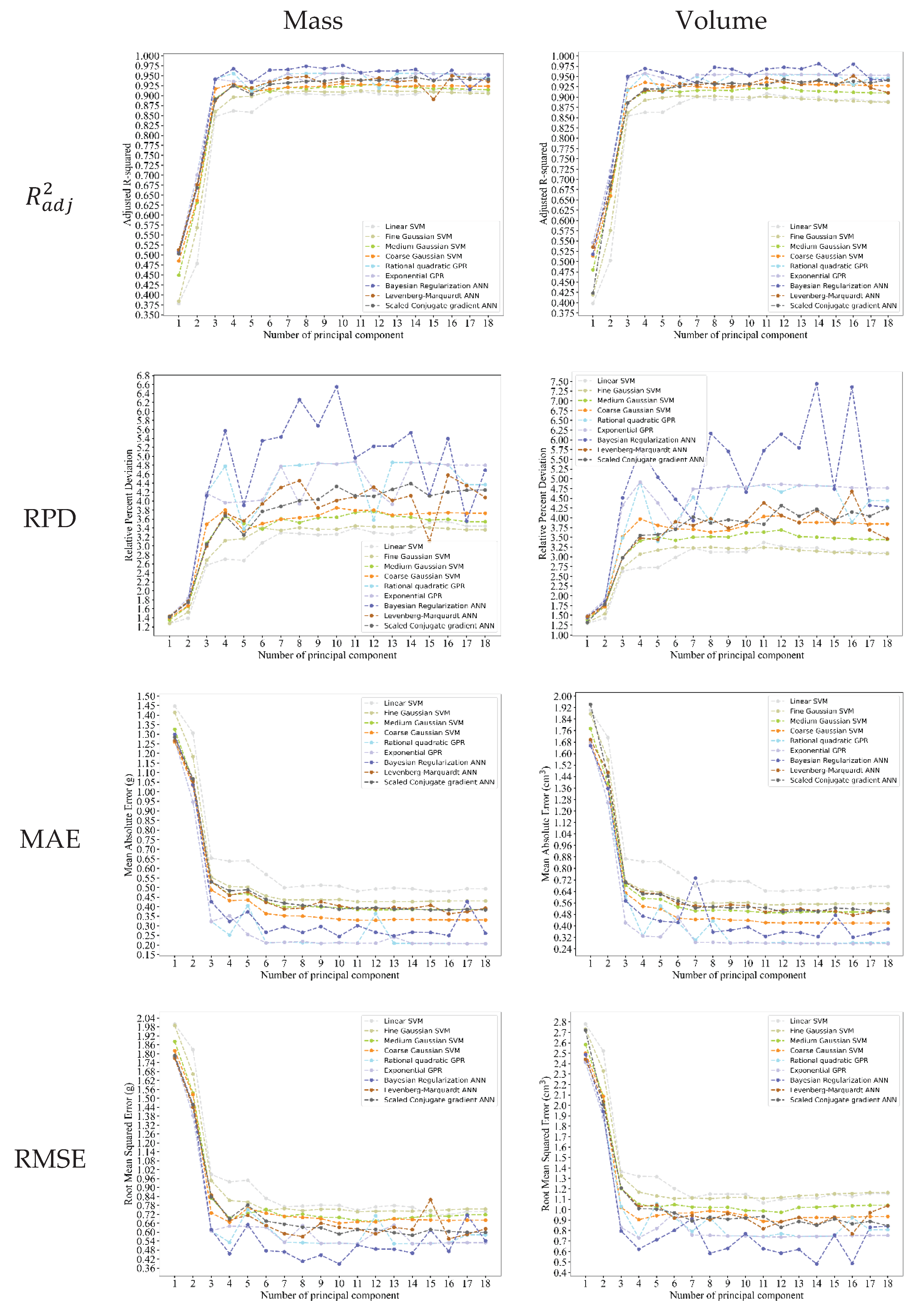
As shown in Figure 12, we plotted a heatmap of the correlation between the Oudemansiella raphanipies parameters and their mass, aimed at exploring the relationship between the parameters and mass, while reducing information redundancy between the features. Furthermore, since volume and mass have a close correlation, the relationship between phenotypic parameters and volume was evaluated. From the Figure 12, it can be seen that the height, width, perimeter, area have a high correlation with the mass and volume. However, there is also a high correlation between height, width, perimeter, and area, indicating some redundancy. Therefore, to explore the impact of nine ML models and the number of the Principal Component Analysis (PCA) components on model performance, we applied the phenotypic data obtained in section 3.4 to evaluate the accuracy of the mass and volume estimation and the results are shown in Figure 13. Whether for mass or volume estimation, as the number of principal components increases, MAE and RMSE all show a downward trend. When the number of principal components reaches 7, the evaluation metrics begin to converge, which indicates a high level of information redundancy among the 18 features.
For mass estimation, the Gaussian kernel in SVM outperforms the linear kernel, especially the Medium Gaussian SVM and Coarse Gaussian SVM, both of which achieved a of 0.92. Additionally, the Medium Gaussian SVM achieved the highest RPD and the lowest RMSE, 3.61 and 0.70g, respectively, while the Coarse Gaussian SVM achieved the lowest MAE of 0.35g. In comparison, the Linear SVM had a of 0.91, RMSE of 0.77g, RPD of 3.30, and MAE of 0.50g. For GPR models, Rational Quadratic GPR and Exponential GPR both had identical , RMSE, RPD, and MAE values of 0.96, 0.53g, 4.78, and 0.21g, respectively. However, Exponential GPR demonstrated more stable performance compared to Rational Quadratic GPR. For Artificial Neural Networks (ANN), the Bayesian Regularization ANN performed the best, with a of 0.97, RMSE of 0.47g, RPD of 5.43, and MAE of 0.29g. Among the models, Exponential GPR had the smallest MAE of 0.21g, while Bayesian Regularization ANN had the highest and RPD, at 0.97 and 5.34, respectively, and the smallest RMSE at 0.47g. For volume estimation, Exponential GPR performed the best, achieving the highest and RPD of 0.95 and 4.74, and the lowest RMSE and MAE of 0.76 cm³ and 0.29 cm³, respectively. Considering both the stability and accuracy of the models for mass and volume estimation, we ultimately select the Exponential GPR with 7 principal components as the model for subsequent mass and volume estimation.
Figure 13.
The evaluated results (, RPD, MAE, RMSE) on the validation set.
3.5. The results Under Different Conditions
3.5.1. Estimation Results of Single Sample at Random States
Since the phenotypic parameters of the same Oudemansiella raphanipies vary when viewed from different perspectives, we selected 24 Oudemansiella raphanipies instance, each with 10 randomly generated states (Dataset 3), to validate the impact of placement state on the Exponential GPR model that obtained in section 3.4. Table 7 shows the estimated mass and volume results of single sample at random states. The manual measurements of mass and volume had average values ranging from 2.20g to 3.40g and from 3.04cm3 ~ 4.70cm3, respectively. Compared with the measured value, the estimated value of mass and volume had an average MAE of 0.26g and 0.34cm3, with an average STD of 0.19g and 0.28cm3, respectively. Moreover, the average CV of mass and volume were 6.81% and 6.94%, which indicated that the Exponential GPR model had robustness on Oudemansiella raphanipies at different states.
3.5.2. Estimation Results of Multiple Samples on One Image at Random States
Although our method demonstrates acceptable performance on individual images of Oudemansiella raphanipies, the number of samples is typically multiple and in random states in real-world assembly lines. Therefore, to validate the practicality of the proposed algorithm in real scenarios, Dataset 4 is selected to simulate the state of Oudemansiella raphanipies on the assembly line and the estimated the mass and volume were shown in Figure 14 and the total error were shown in Table 8.
For S samples, our method achieved an accuracy of over 70% both for mass and volume and a RMSE of 0.590 g and 0.835 cm3, respectively. Moreover, the average MAPE for the mass and volume of S samples was the largest compared to both M and L samples with values of 18.17% and 17.94%, respectively. This is because that although the MAE for the S sample is only 1.454g for mass (2.14cm3 for volume) higher than that of the M sample, the reference value for the former is much smaller than that of the latter, as the S samples have smaller reference mass and volume. For M samples, although the MAPE of mass (volume) is 1.01% (1.11%) higher than L samples, the RMSE between reference mass (volume) and estimated mass (volume) is the lowest. The performance on L samples is the best with a MAPE of 3.21% for mass and 3.66% for volume due to the most regular shape and our extraction method of phenotypic parameters can obtain more accurate data. Despite that, the proposed method showed a MAE of 1.454g and 2.140cm3 for multiple Oudemansiella raphanipies of different grades in one image to estimate the mean mass and volume at single view. Mass and volume estimation were robust at different grades instance. Additionally, as shown in Figure 14 (c) and (d), the violin plot visualizes the relative estimation errors of 10 results for 10 Oudemansiella raphanipies samples at different grades. The width of the violin plot represents the distribution of the data, with a wider section indicating that the estimations are more concentrated at that position. The length of the violin plot represents the degree of dispersion, where a longer instrument body signifies greater instability in the measurement results. It can be reported that the relative error of mass might even exceed 4 g such the No.5 of S samples and the No.7 of L samples, resulting in a low accuracy. Meanwhile, the volume estimation also contains instances with large errors. The large errors imply that these instances will contribute to a greater prediction error for the corresponding images.
3.5.3. Comparison Results of Samples at Different Grades
To further demonstrate the robustness of our method and the consistency of the estimated results, we also statistically analyzed the MAE and CV of the same Oudemansiella raphanipies across different images as shown in Figure 15 and Table 9. For S samples, the CV for both mass and volume estimation are within 5%, which implies the high robustness.
For L samples, it has a MAE with 1.045g and 1.830cm3 and has higher overall CV than S and M samples both for mass and volume, which indicated that the estimated results of L samples have a higher volatility. In addition, the MAPE for the S samples obtains an opposite result with a value of 48.62% for mass and a value of 44.89% for volume, while that of the M and L samples are much lower. This is because the mass and volume variations of the M and L samples are more significant, leading to higher variability in their measurements, resulting in a larger CV. Furthermore, the MAPE is sensitive to the relative impact of errors with respect to the target size. For L samples, it has a larger overall mass and volume, so the same MAE has a smaller relative impact in terms of percentage, leading to a lower MAPE. On the other hand, the shape of the same Oudemansiella raphanipies is not exactly the same on different placement surfaces, leading to variations in the extracted phenotypic parameters, which ultimately affect the estimates of mass and volume.
4. Discussion
Regarding the Oudemansiella raphanipies instance segmentation task, we integrated the NAF module and the PointRend module into FinePoint-ORSeg network to improve the segmentation capabilities and address the issue of rough target boundaries during inference. The results showed a similar performance to other state-of-art works based on DL (Table 5) which reported an AP results at 0.831. Instance segmentation tasks were prominent at large scale, despite slightly better for IoU50 (AP50 = 0.984) than for IoU75 (AP75 = 0.930). The authors attribute the better instance segmentation of Oudemansiella raphanipies on large samples to the fact that they are larger and the NAF block maintains nonlinear expressive power while circumventing gradient-related issues inherent in traditional activation functions, thereby enhancing the model's adaptability to large-scale targets.
The main contribution of this work is the phenotypic parameters extraction algorithms and the use of ML to estimate the Oudemansiella raphanipies (mass and volume) even in the presence of multiple targets. The results (Table 6) show that the phenotypic parameters extraction algorithm was able to robustly obtain the features such as CD (MAE = 1.01mm), CH (MAE = 0.73mm), SD (MAE = 1.30mm) and SH (MAE = 0.58mm). Compared with other state-of-art results that measure CD of Oudemansiella raphanipies [26,27], this study achieved MAE values of between 0.357mm and 0.93mm and is considered as an accurate and acceptable results and achieved. However, it is notable that the error (Table 6) of the number of 1 (MAPE = 13.26%) and 8 (MAPE = 11.39%) of CD, the number of 2 (MAPE = 11.30%) of CH and the number of 7 (MAPE = 10.71%) of SD were significantly higher than other Oudemansiella raphanipies. The main reason are as follows: (1) Error introduced by manual measurement. Since the Oudemansiella raphanipies is a non-rigid object, compression may occur during measurement, leading to an underestimation of the reference value. Additionally, the determination of measurement points manually involves a certain degree of subjectivity. (2) Error introduced by view angle of measurement. Due to the irregular shape of the Oudemansiella raphanipies and the fact that the manual measurement perspective is different from the camera's perspective, there is a discrepancy between the manual measurement and the system's measurement results. (3) Error introduced by our extraction approach. Due to the significant influence of external environmental factors on the shape of the Oudemansiella raphanipies, some instances have large caps but narrow stems, while others have small caps but thick stems. As a result, our segmentation method based on the angle between the stem and cap requires different threshold values for the latter case, which would also cause errors in the phenotypic parameters extraction.
The correlation analysis results show that RLW, roughness, and ARMB have low correlations with mass and volume. Therefore, the performance of nine machine learning models was compared under different numbers of principal components, and finally selected the Exponential GPR as subsequent basic model. Furthermore, the Exponential GPR were applied to evaluate the samples at different states. The experiments show that the CV of instance number 9 and 18 for single samples (Table 6) and the accuracy of image number 5 and 9 for multiple samples (Figure 14 (b)) have an unsatisfactory result. As shown in Figure 16 is the CV of extracted 18 phenotypic parameters of above samples, it can be seen that the Angle and Total Area of No.9 sample have a relatively larger error of 8.97% and 9.12% compared with other features. Moreover, the Opening angle, Perimeter and Total Area also have a relatively larger error. For three grades samples, all of the Opening angle obtains a CV exceed 5% and it indicates a relatively large volatility, and this might be an important reason for the significant difference in the prediction results of the two images.
The phenotypic parameters extracted in this work were obtained with 2D image and calibration at fixed height, which limits the data precision and the number of features. The use of 2.5D or 3D data would provide higher precision for subsequent estimation. However, the Oudemansiella raphanipies is relatively small in size, higher-precision depth cameras or three-dimensional phenotypic extraction methods need to be adopted. In addition, the phenotypes of Oudemansiella raphanipies of different varieties and in different planting environments vary greatly. Therefore, it is urgent to develop an adaptive phenotypic parameter extraction method with high robustness.
5. Conclusion
In our work, a computer vision-based method was proposed for estimating the mass of Oudemansiella raphanipies and the work was divided into three subtask, Oudemansiella raphanipies region extraction, phenotypic parameter extraction and mass and volume estimation. First, a DL method named FinePoint-ORSeg, which integrates the NAF block and PointRend module, was proposed to obtain the basis data for subsequent work and the results show that the improved DL method achieved a highest AP50 of 0.984 compared with other instance segmentation networks. Second, a shape prior-based cap-stem segmentation approach was proposed to calculate the phenotypic parameter and an average MAE of 1.10 mm, 0.73 mm, 1.30 mm, 0.58 mm were achieved for the diameter and height of cap, diameter and height of stem, respectively. Finally, the ML method utilized PCA algorithm to reduce the dimension of the phenotypic parameter features and finally predicted the mass and volume of Oudemansiella raphanipies. To validate the robustness of our method, the image of single and multiple Oudemansiella raphanipies were applied to test the error and the results show that for the same Oudemansiella raphanipies measured 10 times, the average coefficient of variation (CV) for mass and volume are 6.81% and 6.94%, respectively. Meanwhile, the MAPE of different grades of multiple samples in one image are 8.53% and 8.46% for mass and volume, respectively. This can provide a data foundation and technical support for the post-harvest packaging of Oudemansiella raphanipies.
Despite our mass and volume estimation approach has achieved some results, it still has limitations. For instance, our method divides the work into three subtasks but each sub-task will introduce systematic errors, which increases the difficulty of accurately predicting mass and volume. Future work should consider using a single-stage method to reduce these errors.
Author Contributions
Hua Yin: Conceptualization, Writing – review & editing, Supervision; Danying Lei: Data curation, Methodology, Formal analysis, Writing – original draft; Anping Xiong: Conceptualization ,Lu Yuan: Data curation, Methodology;Minghui Chen: Conceptualization, Methodology; Yilu Xu: Conceptualization, Methodology; Hui Xiao: Conceptualization; Yinglong Wang: Supervision, Project administration, Writing – review & editing; Quan Wei: Methodology, Project administration, Writing – review & editing.
Funding
The work is supported by the National Natural Science Foundation of China (No. 62362039), the Jiangxi Provincial Natural Science Foundation (No.20242BAB25081).
Data Availability Statement
Given that the data used in this study were self-collected, the dataset is being further improved. Thus, the dataset is unavailable at present.
Acknowledgments
Special thanks to the reviewers for their valuable comments.
Conflicts of Interest
The authors declare no conflict of interest.
References
- Yin, H.; Yi, W.; Hu, D. Computer vision and machine learning applied in the mushroom industry: A critical review. Comput. Electron. Agric. 2022, 198, 107015. [CrossRef]
- Yin, H.; Xu, J. ; Wang, Y.; Hu, D.; Yi, W. A novel method of situ measurement algorithm for Oudemansiella Raphanipies caps based on YOLOv4 and distance filtering. Agronomy. 2022, 13, 134. [CrossRef]
- Koc, A.B. Determination of watermelon volume using ellipsoid approximation and image processing. Postharvest Biology and Technology. 2007, 45(3), 366-371. [CrossRef]
- Iqbal, S.M.; Gopal, A.; Sarma, A. Volume estimation of apple fruits using image processing. 2011 International Conference on Image Information Processing. 2011, 1-6. [CrossRef]
- Siswantoro, J.; Hilman, M.; Widiasri, M. Computer vision system for egg volume prediction using backpropagation neural network. IOP Conference Series: Materials Science and Engineering. 2017, 273, 012002.
- Widiasri, M.; Santoso, L.P.; Siswantoro, J. Computer Vision System in Measurement of the Volume and Mass of Egg Using the Disc Method. IOP Conference Series: Materials Science and Engineering. 2019, 703, 012050.
- Siswantoro, J.; Asmawati, E.; Siswantoro, M.Z. A rapid and accurate computer vision system for measuring the volume of axi-Symmetric natural products based on cubic spline interpolation. Journal of Food Engineering. 2022, 333, 111139. [CrossRef]
- Huynh, T.; Tran, L. ; Dao, S. Real-time size and mass estimation of slender axi-Symmetric fruit/vegetable using a single top view image. Sensors. 2020, 20, 5406. [CrossRef]
- Tabatabaeefar, A.; Rajabipour, A. Modeling the mass of apples by geometrical attributes. Scientia Horticulturae. 2005, 105, 373-382. [CrossRef]
- Lorestani, A.N.; Tabatabaeefar, A. Modelling the mass of kiwi fruit by geometrical attributes. Scientia Horticulture. 2006, 105:373-382.
- Lee, J.; Nazki, H.; Baek, J., Hong; Y., Lee, M. Artificial intelligence approach for tomato detection and mass estimation in precision agriculture. Sustainability. 2020, 12, 9138. [CrossRef]
- Jang, S.H.; Moon, S.P.; Kim, Y.J.; Lee, S.-H. Development of potato mass estimation system based on deep learning. Applied sciences. 2023, 13, 2614. [CrossRef]
- He, K.; Gkioxari, G.; Dollár, P.; Girshick, R. Mask R-CNN. Proceedings of the IEEE international conference on computer vision, pp. 2017, 2961-2969. [CrossRef]
- Liu, C.; Feng, Q.; Sun, Y.; Li, Y.; Ru, M.; Xu, L. Yolactfusion: an Instance segmentation method for rgb-nir multimodal image fusion based on an attention mechanism. Comput. Electron. Agric. 2023, 213, 108186. [CrossRef]
- Wang, X.; Zhang, R.; Kong, T.; Li, L.; Shen, C. Solov2: dynamic and fast Instance segmentation. Advances in Neural information processing systems. 2020, 33, 17721-17732.
- Liu, Z.; Lin, Y. ; Cao, Y. ; Hu, H. ; Wei, Y. ; Zhang, Z. ; Lin, S. ; Guo, B. Swin transformer: Hierarchical vision transformer using shifted windows. Proceedings of the IEEE/CVF international conference on computer vision, pp. 2021, 10012-10022. [CrossRef]
- Yang, S.; Zheng, L. ; Yang, H.; Zhang, M.; Wu, T.; Sun, S.; Tomasetto, F.; Wang, M. A synthetic datasets based instance segmentation network for high-throughput soybean pods phenotype investigation. Expert systems with applications. 2022, 192, 116403. [CrossRef]
- Li, S.; Yan, Z.; Guo, Y.; Su, X.; Cao, Y.; Jiang, B.; Yang, F.; Zhang, Z.; Xin, D.; Chen, Q. Spm-Is: An auto-algorithm to acquire a mature soybean phenotype based on instance segmentation. The Crop Journal. 2022, 10, 1412-1423. [CrossRef]
- Sapkota, R.; Ahmed, D.; Karkee, M. Comparing YOLOv8 and Mask R-CNN for instance segmentation in complex orchard environments. Artificial Intelligence in Agriculture. 2024, 13, 84-99. [CrossRef]
- Chen, Z.; Cai, Y.; Liu, Y.; Liang, Z.; Chen, H.; Ma, R.; Qi, L. Towards end-to-end rice row detection in paddy fields exploiting two-pathway instance segmentation. Comput. Electron. Agric. 2025, 231, 109963. [CrossRef]
- He, H.; Ma, X.; Guan, H. A calculation method of phenotypic traits of soybean pods based on image processing technology. Ecological Informatics. 2022, 69, 101676. [CrossRef]
- Liu, R.; Huang, S. ; New, Y. ; Xu, S. Automated detection research for number and key phenotypic parameters of rapeseed silique. Chinese Journal of Oil Crop Sciences. 2020, 42. [CrossRef]
- Zhu, Y.; Zhang, X.; Shen, Y.; Gu, Q.; Jin, Q.; Zheng, K. High-throughput phenotyping collection and analysis of Flammulina Filiformis based on image recognition technology. Myco. 2021, 40, 3. [CrossRef]
- Kumar, M.; Gupta, S.; Gao, X.Z.; Singh, A. Plant species recognition using morphological features and adaptive boosting methodology. IEEE ACCESS. 2019, 7, 163912-163918. [CrossRef]
- Okinda, C.; Sun, Y.; Nyalala, I.; Korohou, T.; Opiyo, S.; Wang, J.; Shen, M. Egg volume estimation based on image processing and computer vision. Journal of Food Engineering. 2020, 283, 110041. [CrossRef]
- Wang, Y.; Xiao, H.; Yin, H.; Luo, S.; Le, Y.; Wan, J. Measurement of morphology of Oudemansiella Raphanipes based on RGBD camera. Nongye Gongcheng Xuebao/Trans. Chinese Soc. Agric. Eng. 2022, 38, 140-148. [CrossRef]
- Yin, H.; Wei, Q.; Gao, Y.; Hu, H.; Wang, Y. Moving toward smart breeding: A robust amodal segmentation method for occluded Oudemansiella Raphanipes cap size estimation. Comput. Electron. Agric. 2024, 220, 108895. [CrossRef]
- Nyalala, I.; Okinda, C.; Nyalala, L.; Makange, N.; Chao, Q.; Chao, L.; Yousaf, K.; Chen, K. Tomato volume and mass estimation using computer vision and machine learning algorithms: Cherry Tomato Model. Journal of Food Engineering. 2019, 263, 288-298. [CrossRef]
- Saikumar, A.; Nickhil, C.; Badwaik, L.S.; Physicochemical characterization of elephant apple (Dillenia Indica L.) fruit and its mass and volume modeling using computer vision. Scientia Horticulturae. 2023, 314, 111947. [CrossRef]
- Kirillov, A.; Wu, Y.; He, K.; Girshick, R. Pointrend: Image segmentation as rendering. Proceedings of the IEEE/CVF conference on computer vision and pattern recognition. 2020, 9799-9808. https://arxiv.org/abs/1912.08193.
- Chen, L.; Chu, X.; Zhang, X.; Sun, J. Simple baselines for image restoration. European conference on computer vision, pp. 2022, 17-33. [CrossRef]
- Cortes, C.; Vapnik, V. Support-vector networks. Machine Learning. 1995, 20, 273-297. [CrossRef]
- Nyalala, I.; Okinda, C.; Nyalala, L.; Makange, N.; Chao, Q.; Chao, L.; Yousaf, K.; Chen, K. Tomato volume and mass estimation using computer vision and machine learning algorithms: Cherry tomato model. Journal of Food Engineering. 2019, 263, 288-298. [CrossRef]
- Quinonero-Candela, J.; Rasmussen, C.E.; Williams, C.K. Approximation methods for gaussian process regression. Large-Scale Kernel Machines, MIT Press, pp. 2007, 203-223.
- Gonzalez, B.; Garcia, G.; Velastin, S.A.; GholamHosseini, H.; Tejeda, L.; Farias, G. Automated food weight and content estimation using computer vision and AI algorithms. Sensors. 2024, 24, 7660. [CrossRef]
- Sofwan, A.; Sumardi, S.; Ayun, K.Q.; Budiraharjo, K.; Karno, K. Artificial neural network levenberg-marquardt method for environmental prediction of smart greenhouse. 2022 9th International Conference on Information Technology, Computer, and Electrical Engineering (ICITACEE), pp. 2022, 50-54. [CrossRef]
- Sivaranjani, T.; Vimal, S.; AI method for improving crop yield prediction accuracy using ANN. Computer Systems Science & Engineering. 2023, 47. [CrossRef]
- Kayabaşı, A.; Sabancı, K.; Yiğit, E.; Toktaş, A.; Yerlikaya, M.; Yıldız, B. Image processing based ANN with bayesian regularization learning algorithm for classification of wheat grains. 2017 10th International Conference on Electrical and Electronics Engineering (ELECO). 2017, 1166-1170.
- Amraei, S.; Abdanan M.S.; Salari, S. Broiler weight estimation based on machine vision and artificial neural network. British poultry science. 2017, 58, 200-205. [CrossRef]
- Akbarian, S.; Xu, C.; Wang, W.; Ginns, S.; Lim, S. Sugarcane yields prediction at the row level Using a novel cross-validation approach to multi-Year multispectral images. Comput. Electron. Agric. 2022, 198, 107024. [CrossRef]
- Yang, H.I.; Min, S.G.; Yang, J.H.; Eun, J.B.; Chung, Y.B. Mass and volume estimation of diverse kimchi cabbage forms using RGB-D vision and machine learning. Postharvest Biology and Technology. 2024, 218, 113130. [CrossRef]
- Yang, H.I.; Min, S.G.; Yang, J.H.; Lee, M.A.; Park, S.H.; Eun, J.B.; Chung, Y.B. Predictive modeling and mass transfer kinetics of tumbling-assisted dry salting of kimchi cabbage. Journal of Food Engineering. 2024, 361, 111742. [CrossRef]
- Wang, D.; Feng, Z.; Ji, S.; Cui, D. Simultaneous prediction of peach firmness and weight using vibration spectra combined with one-dimensional convolutional neural network. Comput. Electron. Agric. 2022, 201, 107341. [CrossRef]
- Xie, W.; Wei, S.; Zheng, Z.; Chang, Z.; Yang, D.; Developing a stacked ensemble model for predicting the mass of fresh carrot. Postharvest Biology and Technology. 2022, 186, 111848. [CrossRef]
- Luo, S.; Tang, J.; Peng, J.; Yin, H.;. A novel approach for measuring the volume of pleurotus eryngii based on depth camera and improved circular disk method. Scientia Horticulturae. 2024, 336, 113382. [CrossRef]
Figure 1.
Diagram of the imaging system.
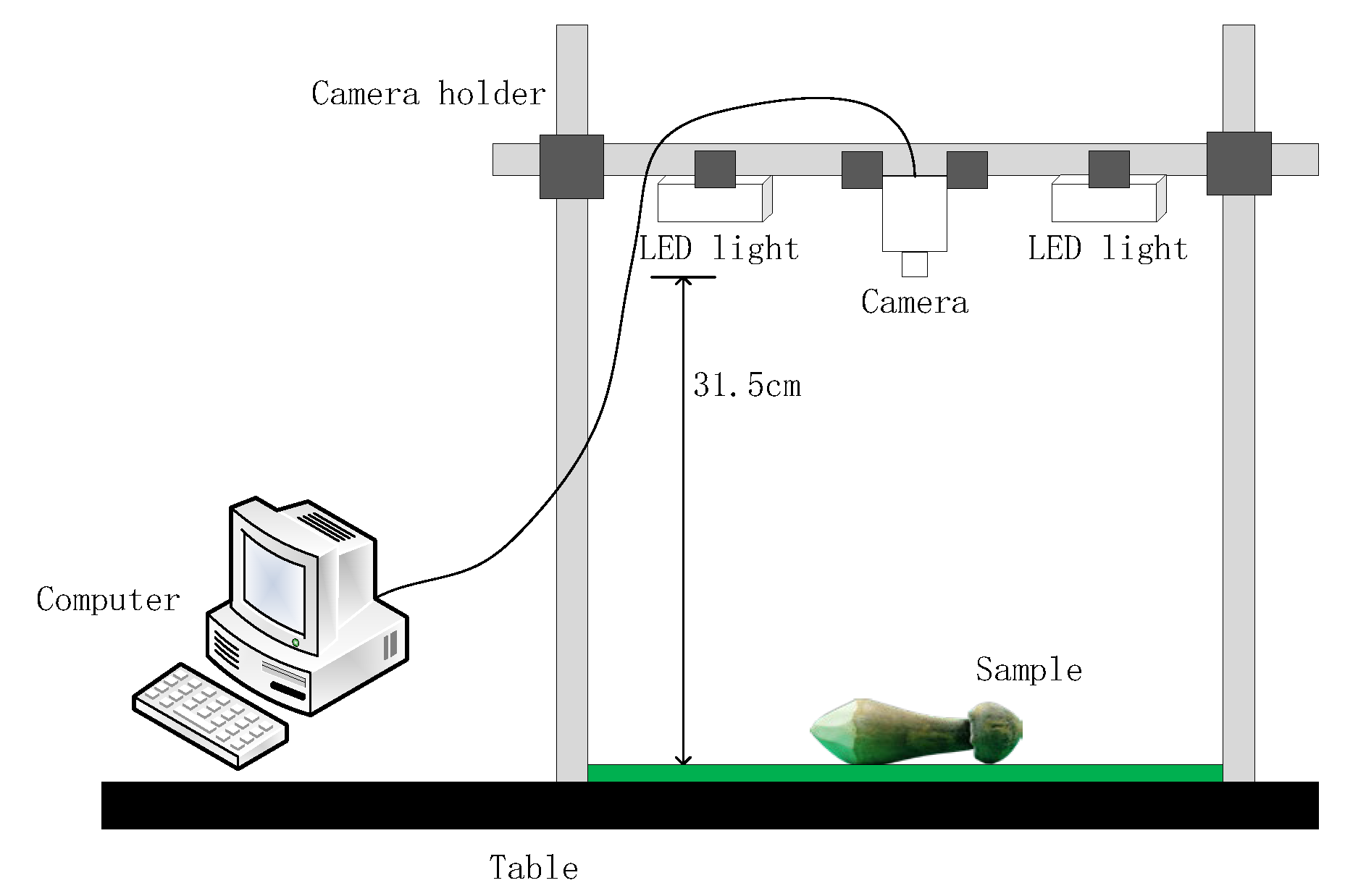
Figure 2.
4 datasets used in our work. (a) Dataset 1, used to train the DL model to segment the multiple Oudemansiella raphanipies samples. (b) Dataset 2, utilized to build the ML model to estimate the mass of Oudemansiella raphanipies. (c) Dataset 3, used to evaluate the estimation effect of the mass of individual Oudemansiella raphanies under different placement states. (d) Dataset 4, used to verify the mass of multiple Oudemansiella raphanipies with different grades.
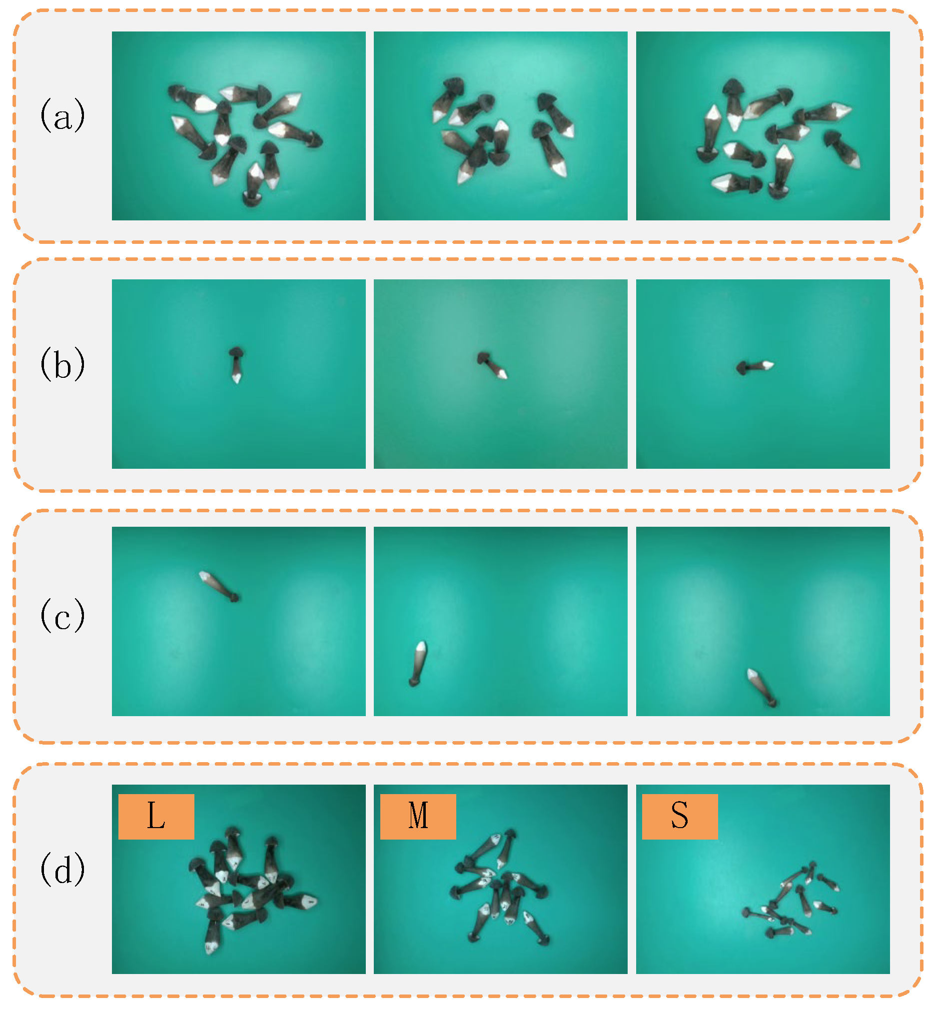
Figure 3.
Examples of different grades of Oudemansiella raphanipes.
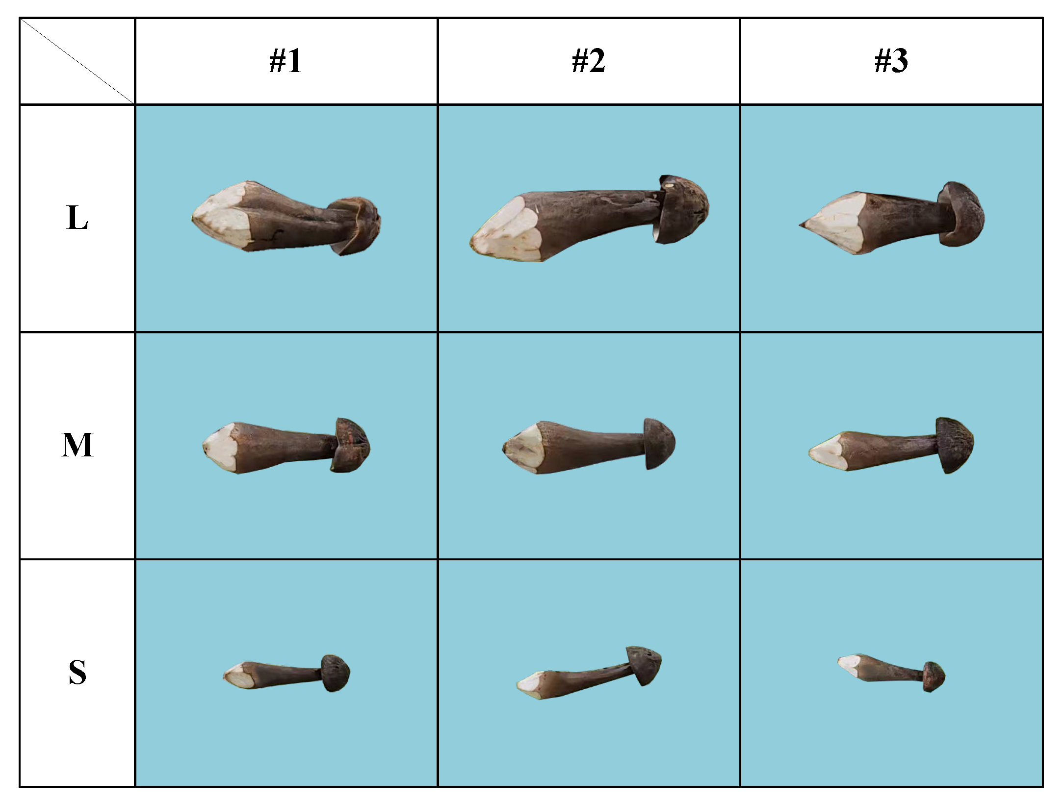
Figure 4.
Pipeline of our method.
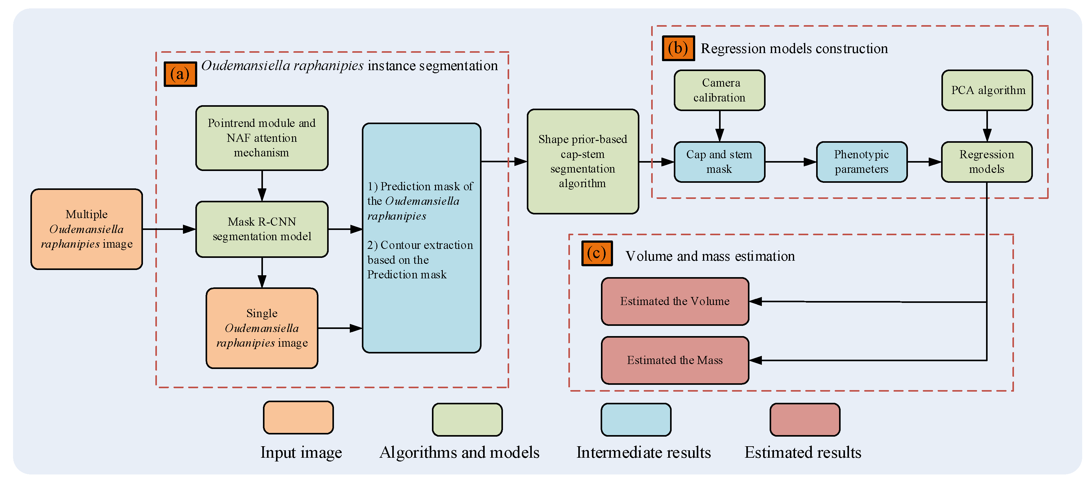
Figure 5.
The schematic diagram of segmentation by FinePoint-ORSeg module.
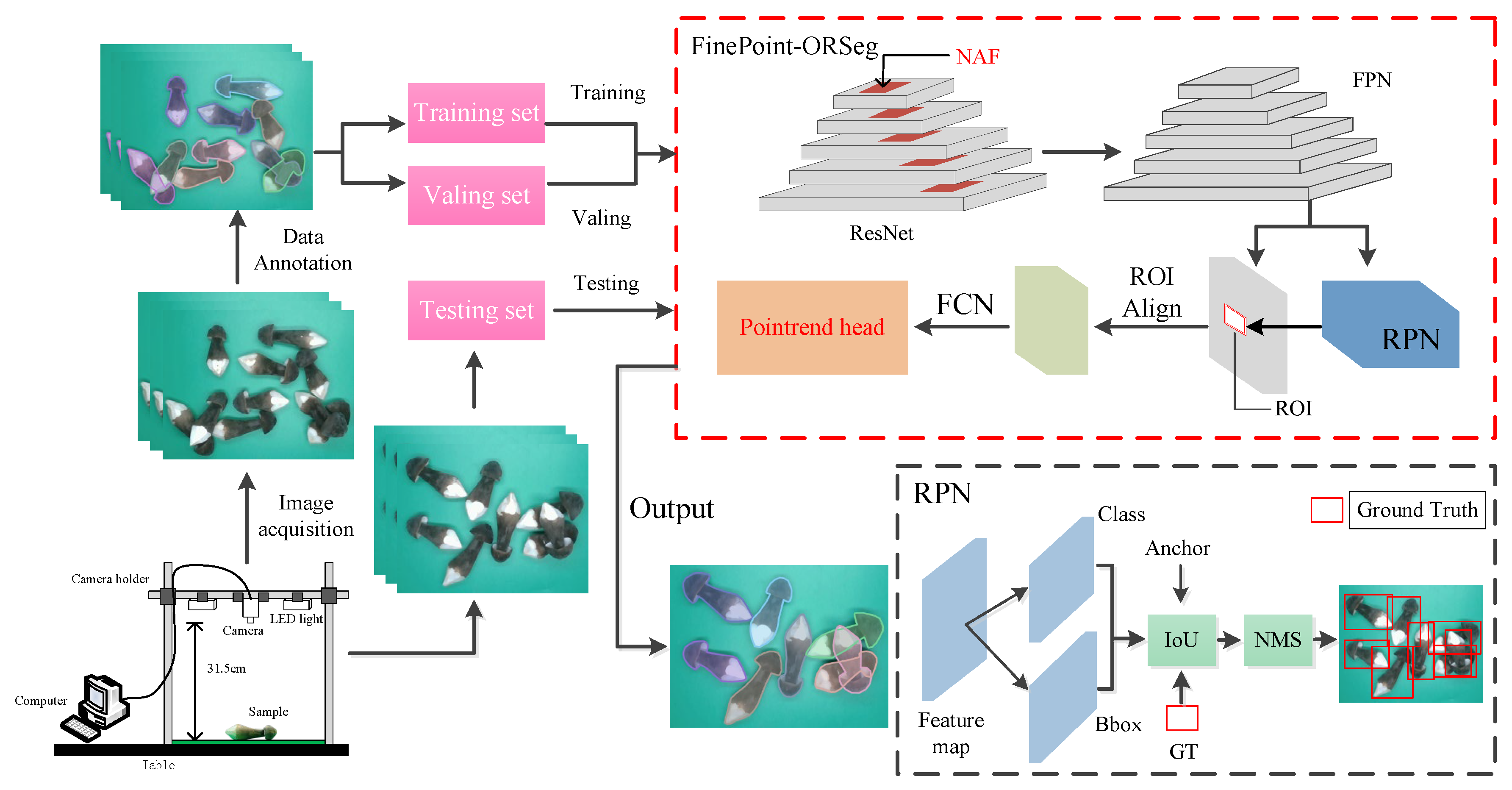
Figure 7.
Flow chart of cap-stem segmentation.
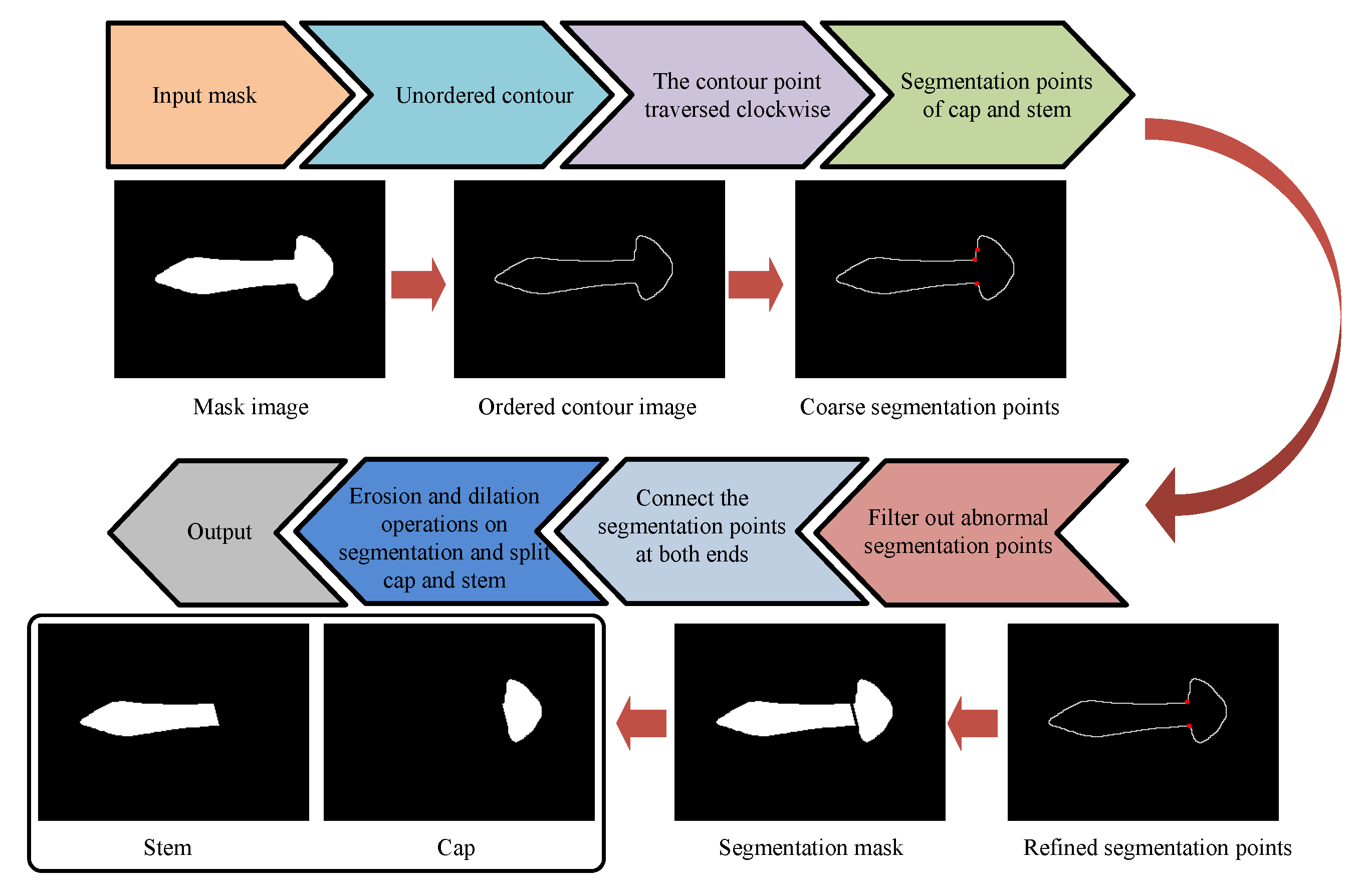
Figure 8.
The revising process of the bounding box of cap and stem.
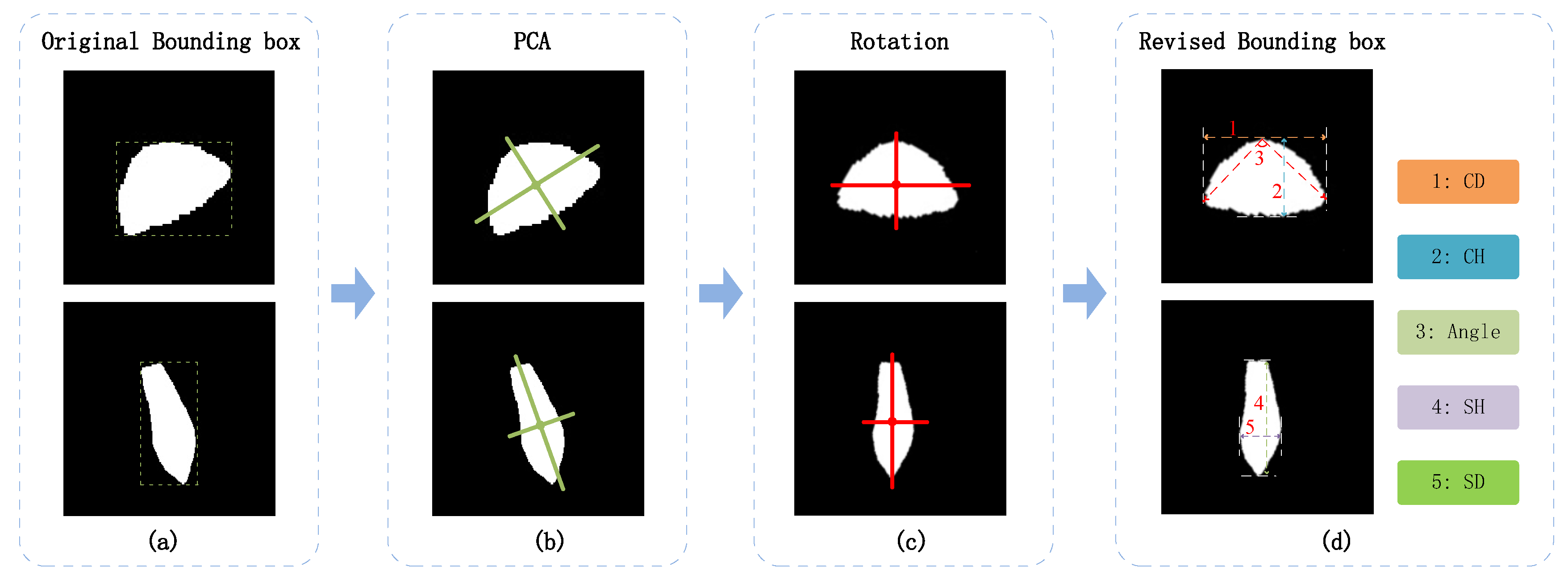
Figure 9.
Relationships of mass and volume between ground-truth and prediction.
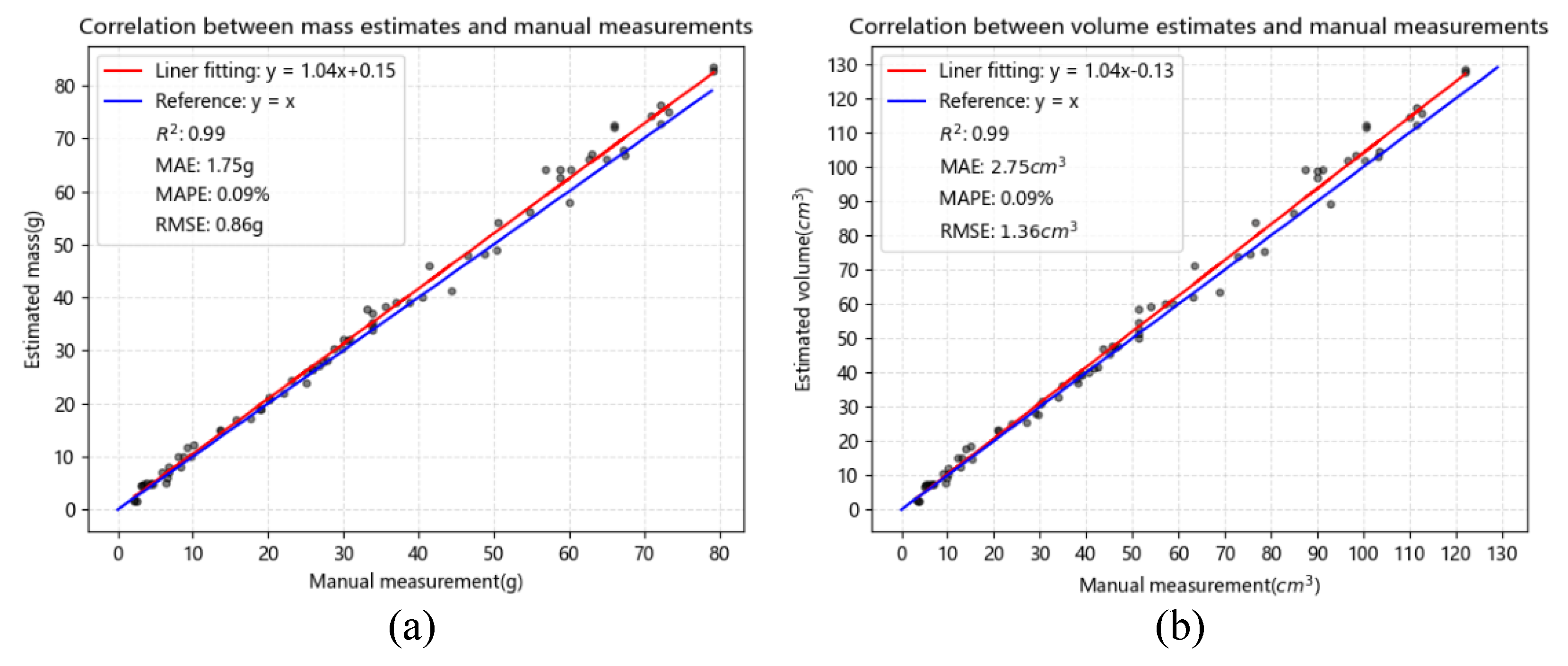
Figure 10.
Loss curves.
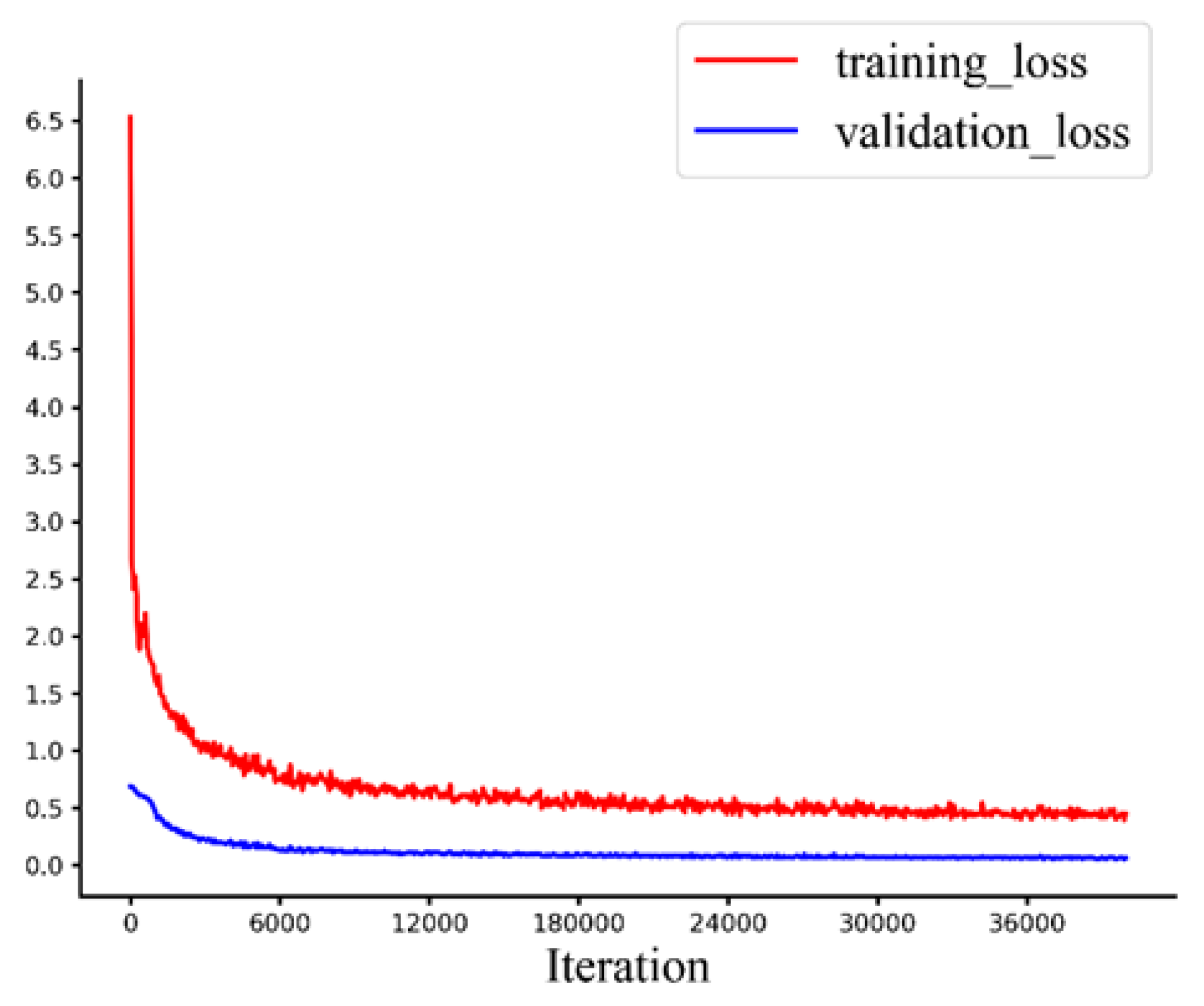
Figure 11.
Segmentation visualization results of FinePoint-ORSeg model. Different colors represent different Oudemansiella raphanipies instance and the colors are generated randomly.
Figure 11.
Segmentation visualization results of FinePoint-ORSeg model. Different colors represent different Oudemansiella raphanipies instance and the colors are generated randomly.
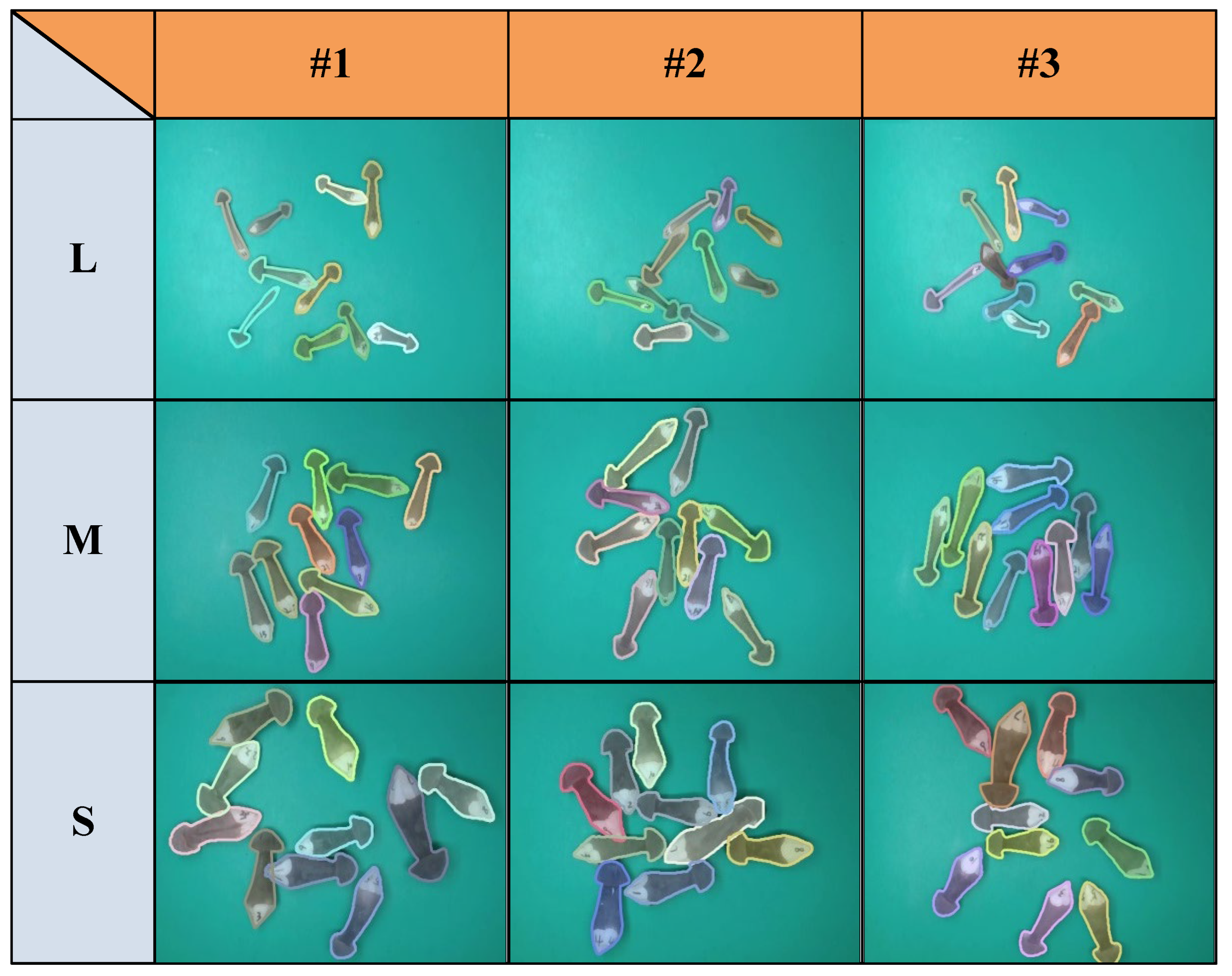
Figure 12.
The correlations of characteristic parameters with mass and volume.
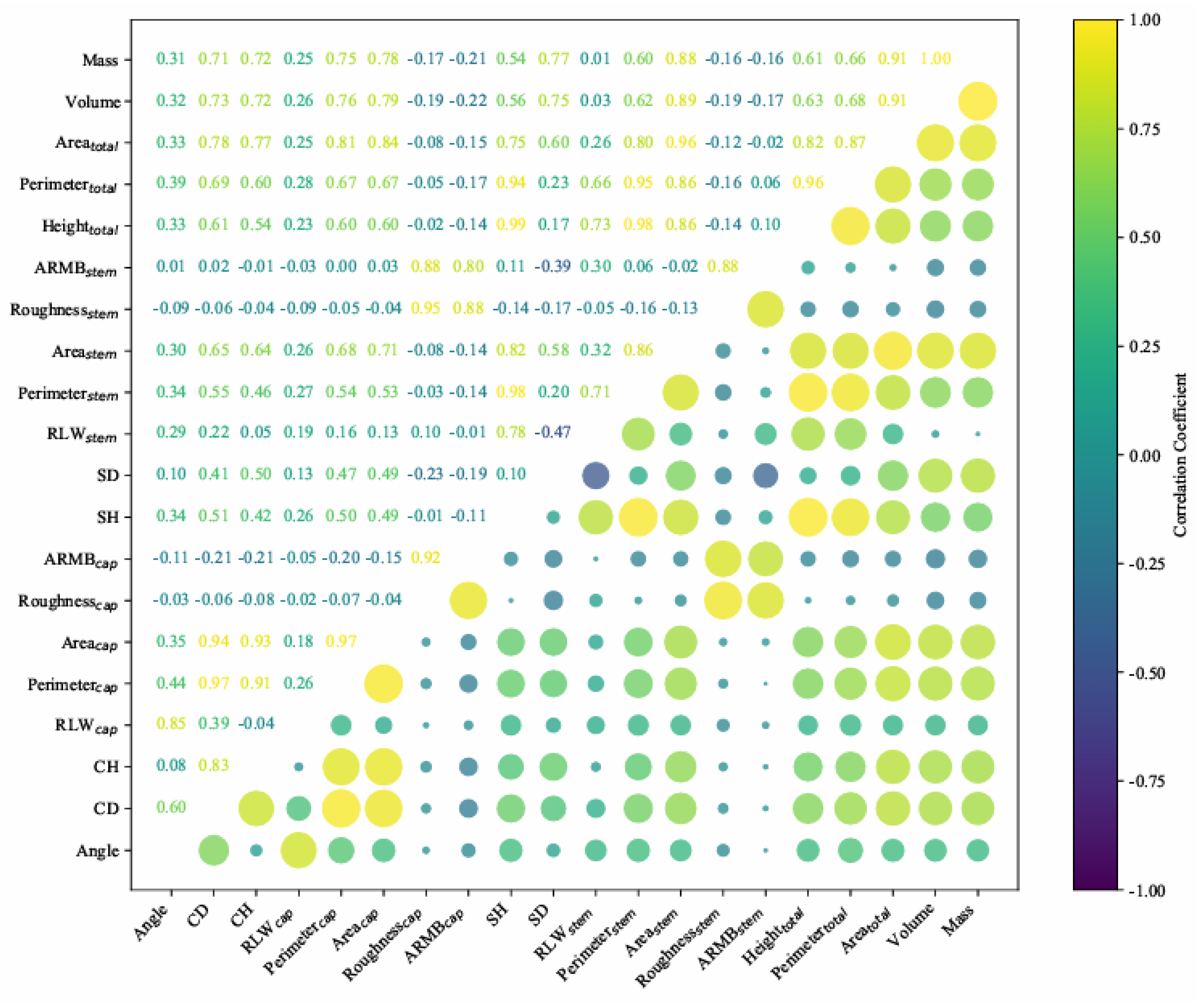
Figure 14.
The results of different grades samples between estimated results and manual measurement. (a) Rows 1, 2, 3 represent the multiple samples of different grades. Columns 1, 2, 3 represent three numbered image examples. (b) The line chart represents the average accuracy of the estimation results in 30 images, and the bar chart represents the average absolute error of the estimation results in 30 images. Blue represents small samples, pink represents medium samples, and yellow represents large samples. (c) The relative errors of mass between estimation and reference measurements. (d) The relative errors of volume between estimation and reference measurements.
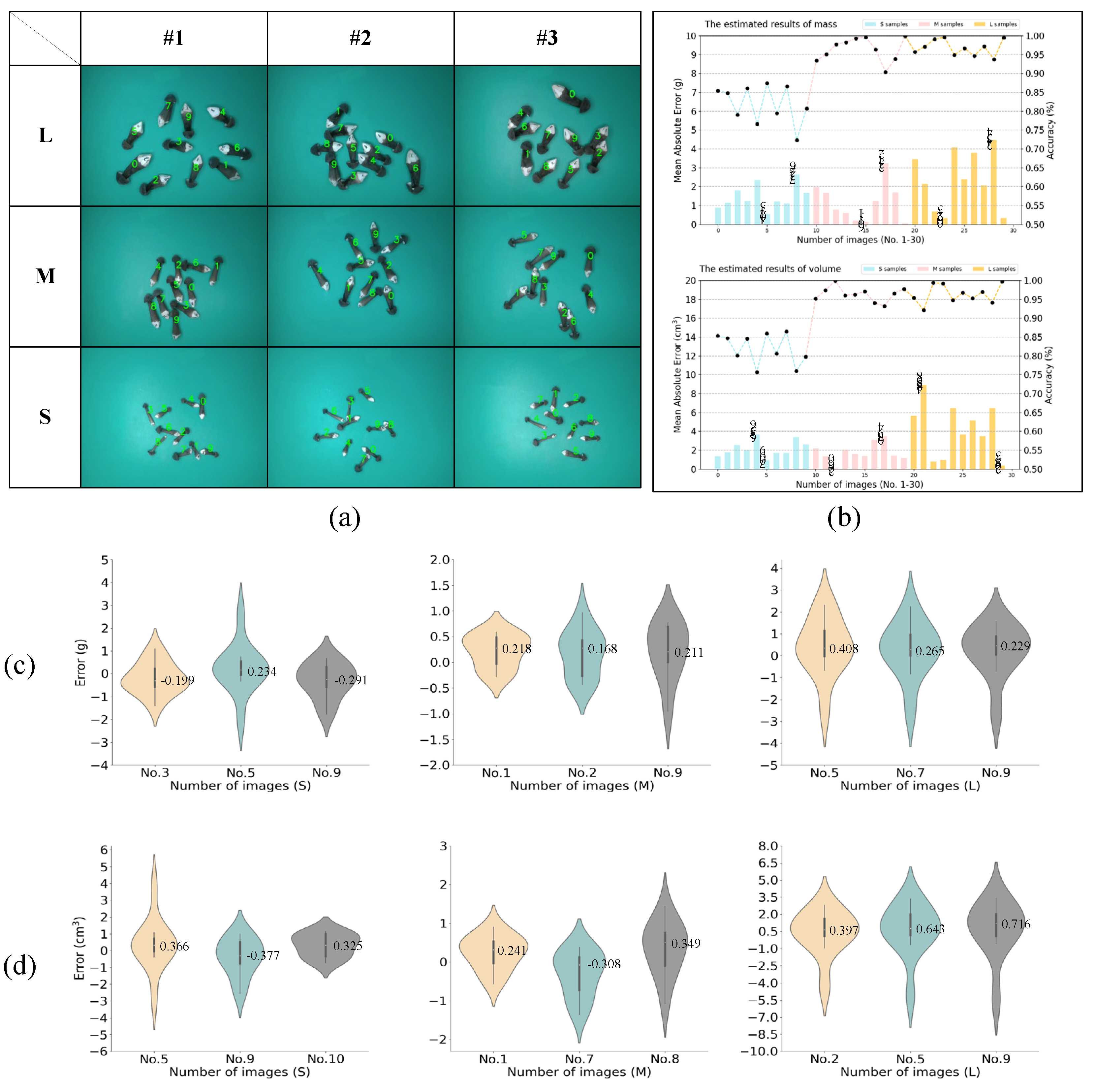
Figure 15.
Estimated results of mass and volume of each Oudemansiella raphanipies on 10 different images. The line chart represents the coefficient of variation of each Oudemansiella raphanipies of different grades on 10 different images, and the bar chart represents the average absolute error of each Oudemansiella raphanipies of different grades on 10 different images. Blue represents small samples, pink represents medium samples, and yellow represents large samples.
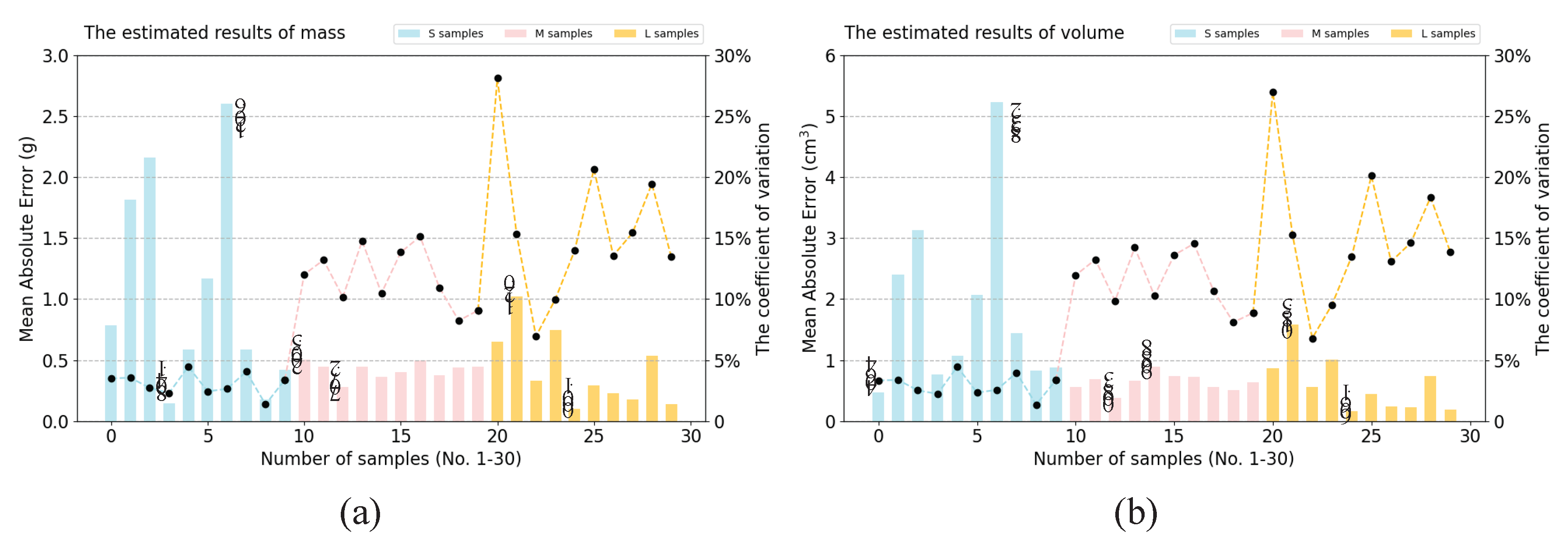
Figure 16.
The CV of 18 features that extracted by our method. No.9 and No.18 (in Table 7) are the single samples measured 10 times at different states, while the S, M, L samples are the CV of the two images with the largest and the smallest errors.
Figure 16.
The CV of 18 features that extracted by our method. No.9 and No.18 (in Table 7) are the single samples measured 10 times at different states, while the S, M, L samples are the CV of the two images with the largest and the smallest errors.
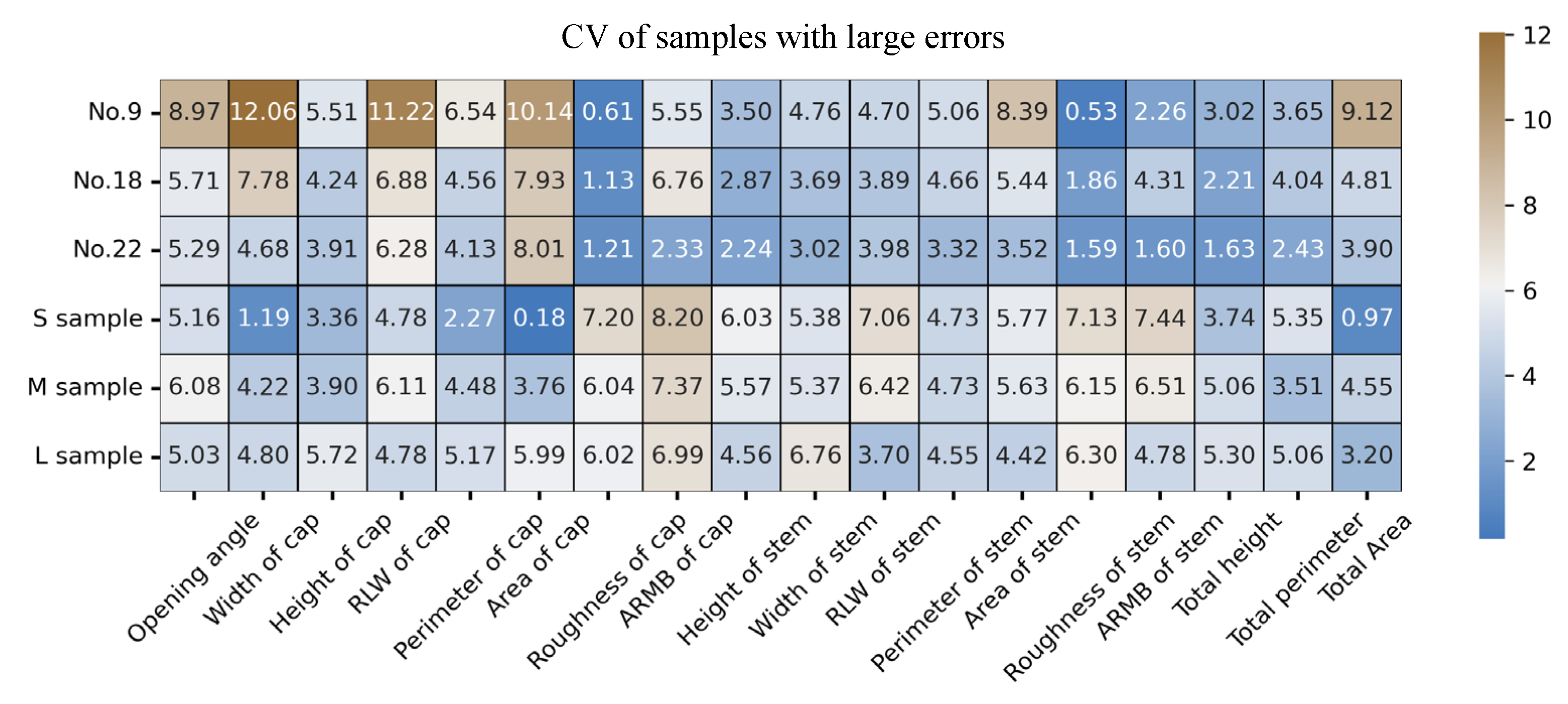
Table 2.
The property descriptions of the GPR and SVR kernels.
| Models | Kernel equations |
| Linear SVM | |
| Fine Gaussian SVM Medium Gaussian SVM Coarse Gaussian SVM |
|
| Rational Quadratic GPR | |
| Exponential GPR | |
| Bayesian Regularization ANN | n-11-2 layers |
| Levenberg-Marquardt ANN | n-11-2 layers |
| Scaled Conjugate gradient ANN | n-11-2 layers |
| Note: σ is the dimensional feature-space scale, is the decay exponent, is the length scale. | |
Table 3.
Evaluation metrics.
| Tasks | Evaluation metrics | Equations |
| Instance segmentation | The average precision () |
|
| Note: TP represents the number of samples that the model correctly predicted as positive examples, FP represents the number of samples that the model wrongly predicted as positive examples, and FN represents the number of samples that the model wrongly predicted as negative examples. | ||
| Phenotypic parameter extraction | Mean absolute error (MAE) | |
| Mean absolute percentage error (MAPE) | ||
| Note: the n refers to the number of samples, represent the manual measurements, and the represent the estimated measurements. | ||
| Regression model | Adjusted () |
|
| Ratio of performance to deviation (RPD) |
|
|
| Mean absolute error (MAE) | ||
| Root mean square error () | ||
| Note: the n refers to the number of samples, represents the number of independent variables, represent the manual measurements, and the represent the estimated measurements. | ||
| Mass evaluation under different conditions | Mean absolute percentage error () | |
| Coefficient of variation () |
|
|
| Note: the n refers to the number of samples, represent the manual measurements, and the represent the estimated measurements, represent the average predicted values. | ||
Table 4.
Table 4. The results of ablation experiment. Bold represents the best result.
| ID | PointRend | NAF | AP | AP50 | AP75 | APs |
| 1 | - | - | 0.811 | 0.977 | 0.911 | 0.857 |
| 2 | √ | - | 0.813 | 0.975 | 0.921 | 0.843 |
| 3 | - | √ | 0.814 | 0.976 | 0.935 | 0.855 |
| 4 | √ | √ | 0.831 | 0.984 | 0.930 | 0.860 |
Table 5.
Comparison of different instance segmentation network on Oudemansiella raphanipies.
| Method | AP | AP50 | AP75 | APs |
| Mask R-CNN | 0.811 | 0.977 | 0.911 | 0.857 |
| SOLOv2 | 0.818 | 0.973 | 0.917 | 0.857 |
| YOLACT | 0.655 | 0.937 | 0.740 | 0.730 |
| Mask2former | 0.831 | 0.969 | 0.908 | 0.864 |
| TensorMask | 0.798 | 0.966 | 0.908 | 0.830 |
| Mask R-CNN with swin | 0.829 | 0.977 | 0.960 | 0.857 |
| InstaBoost | 0.760 | 0.965 | 0.874 | 0.792 |
| FinePoint-ORSeg | 0.831 | 0.984 | 0.930 | 0.860 |
Table 6.
Table 6. Examples of the extracted phenotypic parameters.
| Parameter | Number | (mm) | (mm) | MAE (mm) | MAPE (%) |
| CD | 1 | 14.9 | 16.88 | 1.98 | 13.26 |
| 2 | 20.6 | 21.88 | 1.28 | 6.19 | |
| 3 | 19.5 | 18.75 | 0.75 | 3.85 | |
| 4 | 20.9 | 21.25 | 0.35 | 1.68 | |
| 5 | 21.4 | 21.88 | 0.48 | 2.22 | |
| 6 | 22.1 | 23.75 | 1.67 | 7.47 | |
| 7 | 25.3 | 25.00 | 0.30 | 1.29 | |
| 8 | 20.2 | 22.50 | 2.30 | 11.39 | |
| 9 | 23.7 | 24.38 | 0.68 | 2.85 | |
| 10 | 25.9 | 26.25 | 0.35 | 1.35 | |
| Average | 21.45 | 22.25 | 1.01 | 5.16 | |
| CH | 1 | 12.7 | 12.50 | 0.20 | 1.58 |
| 2 | 14.6 | 16.25 | 1.65 | 11.30 | |
| 3 | 14.0 | 13.75 | 0.25 | 1.79 | |
| 4 | 15.8 | 16.88 | 1.08 | 6.80 | |
| 5 | 15.5 | 15.63 | 0.13 | 0.80 | |
| 6 | 17.8 | 19.38 | 1.58 | 8.85 | |
| 7 | 15.4 | 15.63 | 0.23 | 1.46 | |
| 8 | 13.1 | 14.38 | 1.28 | 9.73 | |
| 9 | 15.2 | 15.63 | 0.43 | 2.80 | |
| 10 | 12.1 | 12.50 | 0.44 | 3.65 | |
| Average | 14.62 | 15.25 | 0.73 | 4.88 | |
| SD | 1 | 39.1 | 39.38 | 0.28 | 0.70 |
| 2 | 30.9 | 30.63 | 0.28 | 0.89 | |
| 3 | 36.5 | 38.13 | 1.63 | 4.45 | |
| 4 | 41.8 | 43.13 | 1.33 | 3.17 | |
| 5 | 58.6 | 61.88 | 3.28 | 5.59 | |
| 6 | 33.7 | 33.75 | 0.05 | 1.48 | |
| 7 | 33.6 | 30.00 | 3.60 | 10.71 | |
| 8 | 33.1 | 31.25 | 1.85 | 5.59 | |
| 9 | 32.7 | 33.13 | 0.43 | 1.30 | |
| 10 | 37.16 | 36.88 | 0.29 | 0.77 | |
| Average | 37.72 | 37.82 | 1.30 | 3.47 | |
| SH | 1 | 13.1 | 13.75 | 0.65 | 4.96 |
| 2 | 14.9 | 15.63 | 0.725 | 4.87 | |
| 3 | 18.5 | 18.75 | 0.25 | 1.35 | |
| 4 | 18.8 | 19.38 | 0.575 | 3.06 | |
| 5 | 17.5 | 18.13 | 0.625 | 3.57 | |
| 6 | 17.8 | 18.75 | 0.95 | 5.34 | |
| 7 | 12.1 | 11.88 | 0.225 | 1.86 | |
| 8 | 18.1 | 18.75 | 0.65 | 3.59 | |
| 9 | 15.9 | 16.25 | 0.35 | 2.20 | |
| 10 | 18.0 | 18.75 | 0.75 | 4.17 | |
| Average | 16.47 | 17.00 | 0.58 | 3.50 |
Table 7.
Results of the estimated results of single samples at random states. Ref refers to the reference data from manual measurements. APV refers to the average predicted values. STD represents the standard deviation.
Table 7.
Results of the estimated results of single samples at random states. Ref refers to the reference data from manual measurements. APV refers to the average predicted values. STD represents the standard deviation.
|
ID |
Mass | Volume | |||||||||
| Ref (g) | APV (g) | MAE (g) | STD (g) | CV (%) | Ref (cm3) | APV (cm3) | MAE (cm3) | STD (cm3) | CV (%) | ||
| 1 | 3.23 | 3.10 | 0.19 | 0.17 | 5.42 | 4.28 | 4.32 | 0.26 | 0.32 | 7.31 | |
| 2 | 2.20 | 2.15 | 0.14 | 0.17 | 7.92 | 3.04 | 2.93 | 0.20 | 0.22 | 7.62 | |
| 3 | 3.21 | 3.20 | 0.22 | 0.25 | 7.92 | 4.25 | 4.46 | 0.32 | 0.30 | 6.81 | |
| 4 | 3.36 | 3.10 | 0.29 | 0.28 | 9.13 | 4.29 | 4.43 | 0.21 | 0.23 | 5.25 | |
| 5 | 2.37 | 2.45 | 0.17 | 0.19 | 7.59 | 3.55 | 3.46 | 0.28 | 0.28 | 8.16 | |
| 6 | 2.53 | 2.40 | 0.23 | 0.20 | 8.27 | 3.34 | 3.46 | 0.23 | 0.25 | 7.26 | |
| 7 | 2.95 | 2.40 | 0.55 | 0.10 | 4.12 | 3.96 | 3.51 | 0.45 | 0.11 | 3.09 | |
| 8 | 2.72 | 2.70 | 0.08 | 0.10 | 3.84 | 3.45 | 3.65 | 0.25 | 0.26 | 7.02 | |
| 9 | 3.10 | 2.93 | 0.40 | 0.39 | 13.34 | 4.38 | 4.66 | 0.64 | 0.58 | 12.37 | |
| 10 | 3.31 | 3.43 | 0.15 | 0.12 | 3.37 | 4.35 | 4.81 | 0.46 | 0.11 | 2.21 | |
| 11 | 2.92 | 2.57 | 0.35 | 0.14 | 5.40 | 4.20 | 3.70 | 0.49 | 0.15 | 3.95 | |
| 12 | 3.11 | 2.95 | 0.27 | 0.28 | 9.57 | 4.25 | 4.24 | 0.28 | 0.37 | 8.84 | |
| 13 | 3.25 | 2.74 | 0.51 | 0.16 | 5.86 | 4.25 | 4.13 | 0.29 | 0.29 | 7.13 | |
| 14 | 3.08 | 3.08 | 0.14 | 0.15 | 5.03 | 4.24 | 4.29 | 0.22 | 0.29 | 6.67 | |
| 15 | 2.17 | 2.27 | 0.21 | 0.22 | 9.69 | 2.98 | 3.31 | 0.33 | 0.26 | 7.99 | |
| 16 | 3.06 | 2.96 | 0.15 | 0.13 | 4.46 | 4.51 | 4.56 | 0.20 | 0.24 | 5.22 | |
| 17 | 2.35 | 2.12 | 0.19 | 0.12 | 5.71 | 3.37 | 3.29 | 0.22 | 0.23 | 7.01 | |
| 18 | 2.98 | 2.70 | 0.19 | 0.32 | 11.88 | 4.01 | 3.85 | 0.44 | 0.51 | 13.21 | |
| 19 | 2.25 | 2.34 | 0.19 | 0.08 | 3.45 | 3.16 | 3.34 | 0.37 | 0.33 | 9.79 | |
| 20 | 3.34 | 3.12 | 0.32 | 0.29 | 9.17 | 4.25 | 4.51 | 0.34 | 0.30 | 6.61 | |
| 21 | 3.40 | 2.54 | 0.86 | 0.18 | 6.99 | 4.70 | 4.03 | 0.67 | 0.20 | 4.98 | |
| 22 | 3.35 | 3.29 | 0.10 | 0.11 | 3.47 | 4.72 | 4.93 | 0.29 | 0.24 | 4.94 | |
| 23 | 3.17 | 3.05 | 0.16 | 0.15 | 4.85 | 4.64 | 4.36 | 0.29 | 0.22 | 4.94 | |
| 24 | 3.29 | 3.29 | 0.21 | 0.23 | 6.90 | 4.46 | 4.46 | 0.33 | 0.36 | 8.12 | |
| Average | 2.95 | 2.79 | 0.26 | 0.19 | 6.81 | 4.03 | 4.03 | 0.34 | 0.28 | 6.94 | |
Table 8.
Average error of the multiple Oudemansiella raphanipies in one image compared with manual measurement.
Table 8.
Average error of the multiple Oudemansiella raphanipies in one image compared with manual measurement.
| Grade | Total | ||||
| S | M | L | |||
| Number of images | 10 | 10 | 10 | 30 | |
| Mass | RMSE () | 0.590 | 0.493 | 1.323 | 0.802 |
| MAE (g) | 1.454 | 1.323 | 2.367 | 1.714 | |
| MAPE (%) | 18.17% | 4.22% | 3.21% | 8.53% | |
| Volume | RMSE () | 0.835 | 0.757 | 2.327 | 1.306 |
| MAE () | 2.140 | 1.796 | 4.713 | 2.703 | |
| MAPE (%) | 17.94% | 3.77% | 3.66% | 8.46% | |
Table 9.
Average error of the each Oudemansiella raphanipies in different images compared with manual measurement.
Table 9.
Average error of the each Oudemansiella raphanipies in different images compared with manual measurement.
| Grade | Total | ||||
| S | M | L | |||
| Number of samples | 10 | 10 | 10 | 30 | |
| Mass | RMSE () | 0.390 | 0.494 | 1.083 | 0.656 |
| MAE (g) | 0.422 | 0.421 | 1.045 | 0.629 | |
| MAPE (%) | 48.62% | 12.76% | 13.97% | 25.12% | |
| Volume | RMSE () | 0.556 | 0.752 | 1.884 | 1.064 |
| MAE () | 0.601 | 0.634 | 1.830 | 1.022 | |
| MAPE (%) | 44.89% | 12.76% | 15.18% | 24.28% | |
Disclaimer/Publisher’s Note: The statements, opinions and data contained in all publications are solely those of the individual author(s) and contributor(s) and not of MDPI and/or the editor(s). MDPI and/or the editor(s) disclaim responsibility for any injury to people or property resulting from any ideas, methods, instructions or products referred to in the content. |
© 2025 by the authors. Licensee MDPI, Basel, Switzerland. This article is an open access article distributed under the terms and conditions of the Creative Commons Attribution (CC BY) license (http://creativecommons.org/licenses/by/4.0/).
Copyright: This open access article is published under a Creative Commons CC BY 4.0 license, which permit the free download, distribution, and reuse, provided that the author and preprint are cited in any reuse.


